Last observation: 2022 (N = 5)
First observation: 1949 (N = 797)
Last data update: 15 oct. 2026, 23:06
Last compile: 16 oct. 2026, 01:26
i_g("bib/insee/compte-d-exploitation.png")
`CNA-2014-CSI` |>
  filter(`SECT-INST` == "S14",
         UNIT_MEASURE == "EUROS_COURANTS",
         OPERATION %in% c("D1", "D4")) %>%
  select_if(~ n_distinct(.) > 1) |>


  year_to_date() |>
  left_join(gdp, by = "date") |>
  ggplot() + geom_line(aes(x = date, y = OBS_VALUE/gdp, color = paste0(OPERATION, " - ", COMPTE))) +
  theme_minimal() +  xlab("") + ylab("") +

  scale_x_date(breaks = as.Date(paste0(seq(1940, 2100, 5), "-01-01")),
               labels = date_format("%Y")) +
  theme(legend.position = c(0.6, 0.6),
        legend.title = element_blank()) +
  scale_y_continuous(breaks = 0.01*seq(0, 2000, 5),
                     labels = percent_format(acc = 1))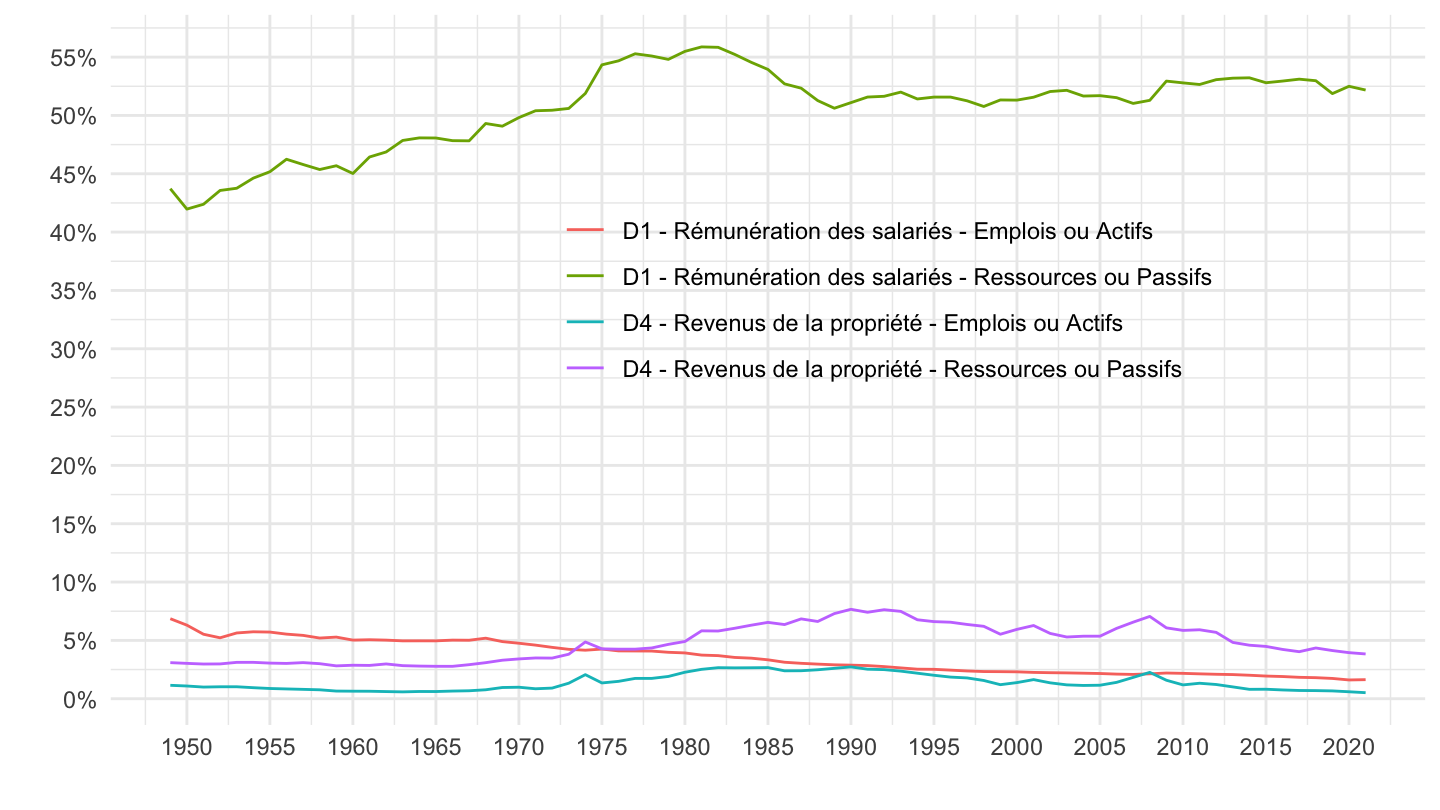
`CNA-2014-CSI` |>
  filter(`SECT-INST` == "S14",
         UNIT_MEASURE == "EUROS_COURANTS",
         OPERATION %in% c("D63", "D631_2010")) |>


  year_to_date() |>
  left_join(gdp, by = "date") |>
  ggplot() + geom_line(aes(x = date, y = OBS_VALUE/gdp, color = OPERATION)) +
  theme_minimal() +  xlab("") + ylab("") +
  scale_color_manual(values = viridis(3)[1:2]) +
  scale_x_date(breaks = as.Date(paste0(seq(1940, 2100, 5), "-01-01")),
               labels = date_format("%Y")) +
  theme(legend.position = c(0.35, 0.9),
        legend.title = element_blank()) +
  scale_y_continuous(breaks = 0.01*seq(0, 2000, 1),
                     labels = percent_format(acc = 1))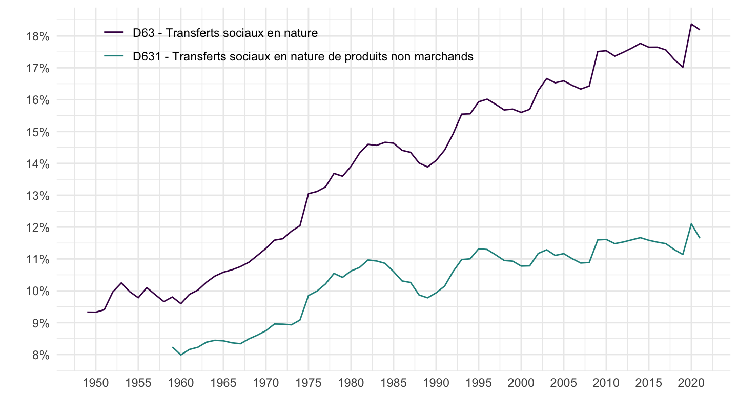
`CNA-2014-CSI` |>
  filter(`SECT-INST` == "S14",
         UNIT_MEASURE == "EUROS_COURANTS",
         OPERATION %in% c("D63", "D631_2010")) |>


  year_to_date() |>
  filter(date >= as.Date("1995-01-01")) |>
  left_join(gdp, by = "date") |>
  ggplot() + geom_line(aes(x = date, y = OBS_VALUE/gdp, color = OPERATION)) +
  theme_minimal() +  xlab("") + ylab("") +
  scale_color_manual(values = viridis(3)[1:2]) +
  scale_x_date(breaks = as.Date(paste0(seq(1940, 2100, 5), "-01-01")),
               labels = date_format("%Y")) +
  theme(legend.position = c(0.3, 0.9),
        legend.title = element_blank()) +
  scale_y_continuous(breaks = 0.01*seq(0, 2000, 1),
                     labels = percent_format(acc = 1))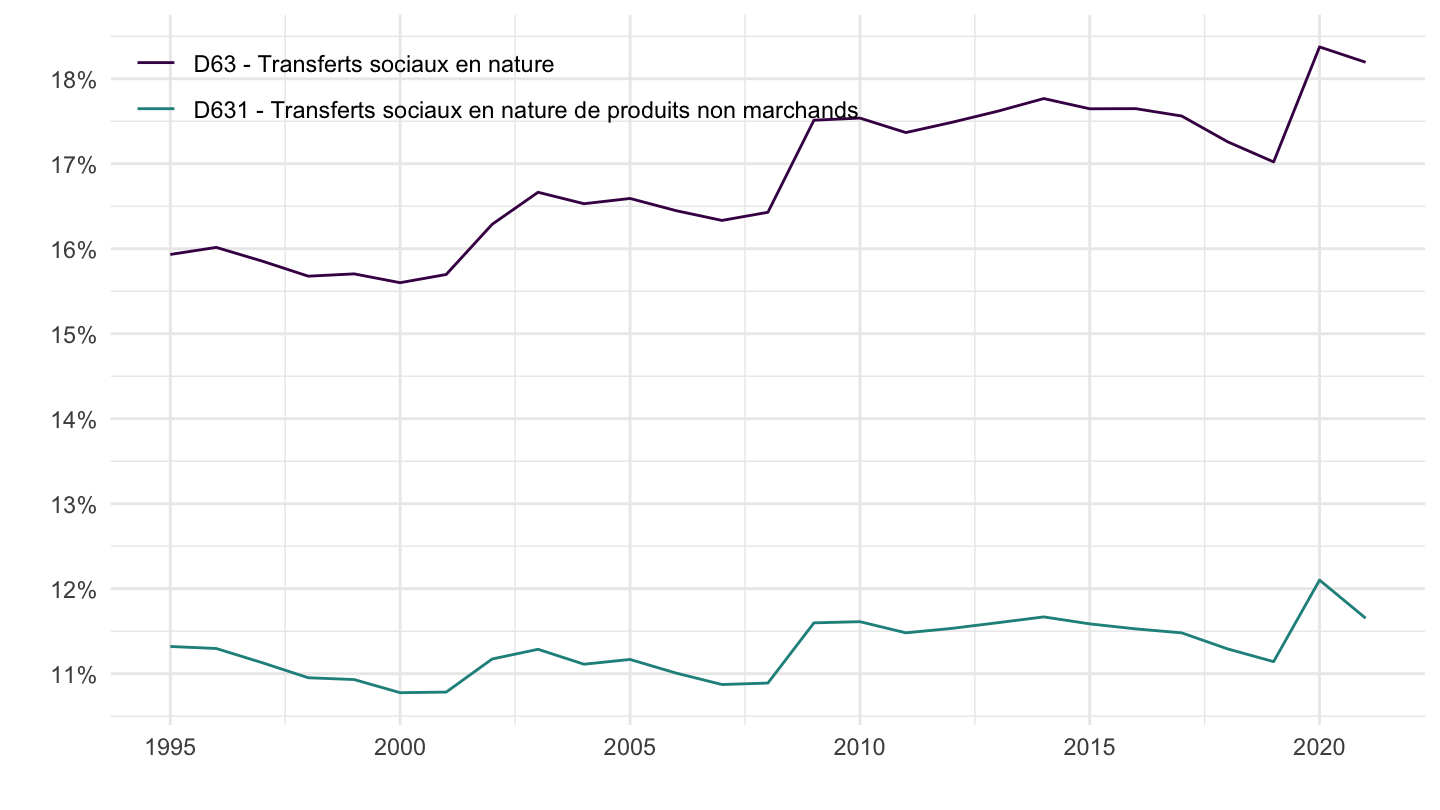
`CNA-2014-CSI` |>
  filter(`SECT-INST` == "S14",
         UNIT_MEASURE == "EUROS_COURANTS",
         OPERATION %in% c("D5")) |>


  year_to_date() |>
  left_join(gdp, by = "date") |>
  ggplot() + geom_line(aes(x = date, y = OBS_VALUE/gdp, color = paste0(OPERATION, " - ", COMPTE))) +
  theme_minimal() +  xlab("") + ylab("") +

  scale_x_date(breaks = as.Date(paste0(seq(1940, 2100, 5), "-01-01")),
               labels = date_format("%Y")) +
  theme(legend.position = c(0.6, 0.6),
        legend.title = element_blank()) +
  scale_y_continuous(breaks = 0.01*seq(0, 2000, 1),
                     labels = percent_format(acc = 1))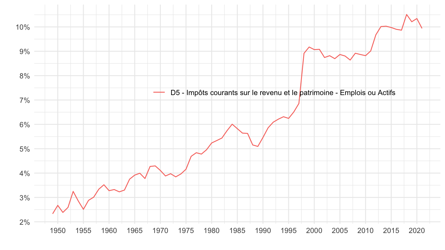
`CNA-2014-CSI` |>
  filter(`SECT-INST` == "S14",
         UNIT_MEASURE == "EUROS_COURANTS",
         OPERATION %in% c("B6G", "B6N", "B7G", "B7N"),
         COMPTE == "EA") |>


  year_to_date() |>
  left_join(gdp, by = "date") |>
  ggplot() + geom_line(aes(x = date, y = OBS_VALUE/gdp, color = paste0(OPERATION, " - ", COMPTE))) +
  theme_minimal() +  xlab("") + ylab("") +

  scale_x_date(breaks = as.Date(paste0(seq(1940, 2100, 5), "-01-01")),
               labels = date_format("%Y")) +
  theme(legend.position = c(0.7, 0.5),
        legend.title = element_blank()) +
  scale_y_continuous(breaks = 0.01*seq(0, 2000, 5),
                     labels = percent_format(acc = 1))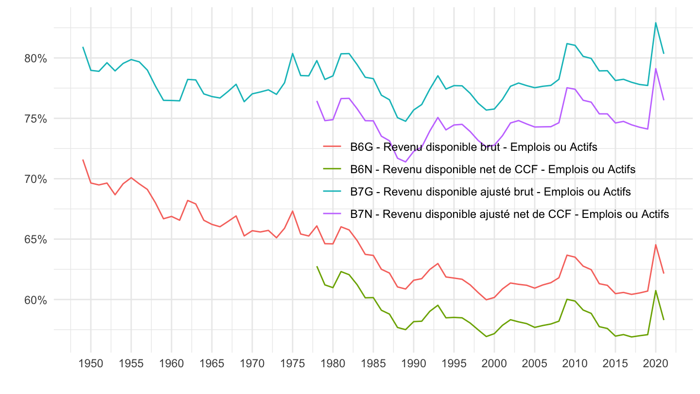
`CNA-2014-CSI` |>
  filter(`SECT-INST` == "S14",
         UNIT_MEASURE == "EUROS_COURANTS",
         OPERATION %in% c("B6G", "B6N", "B7G", "B7N"),
         COMPTE == "EA") |>


  year_to_date() |>
  filter(date >= as.Date("1995-01-01")) |>
  left_join(gdp, by = "date") |>
  ggplot() + geom_line(aes(x = date, y = OBS_VALUE/gdp, color = paste0(OPERATION, " - ", COMPTE))) +
  theme_minimal() +  xlab("") + ylab("") +

  scale_x_date(breaks = as.Date(paste0(seq(1940, 2100, 5), "-01-01")),
               labels = date_format("%Y")) +
  theme(legend.position = c(0.6, 0.5),
        legend.title = element_blank()) +
  scale_y_continuous(breaks = 0.01*seq(0, 2000, 5),
                     labels = percent_format(acc = 1))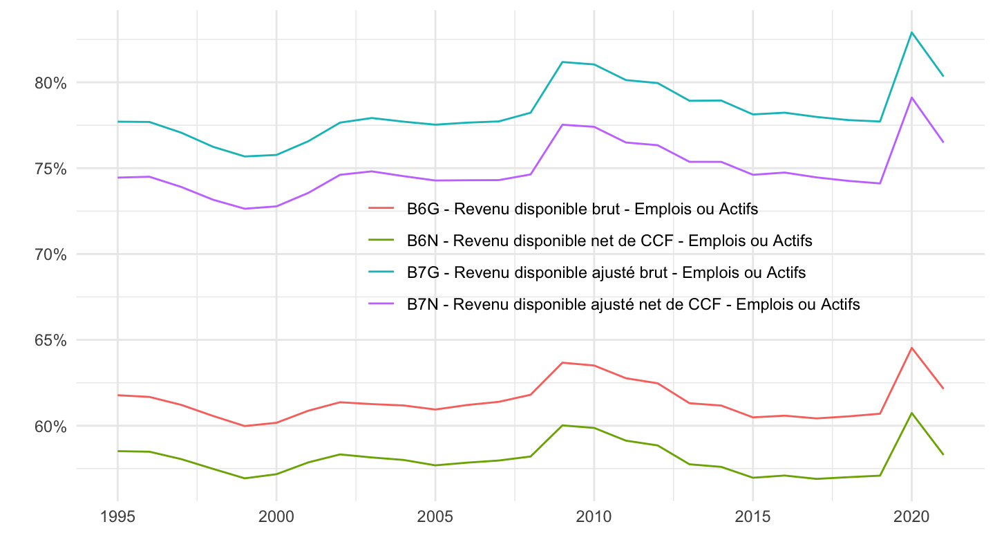
`CNA-2014-CSI` |>

  filter(`SECT-INST` %in% c("S11", "S12", "S14", "S13"),
         OPERATION %in% c("B1G")) |>
  year_to_date() |>
  select(date, `SECT-INST`, `SECT-INST`, OBS_VALUE, UNIT_MEASURE) |>
  ggplot() + geom_line(aes(x = date, y = OBS_VALUE/1000, color = `SECT-INST`)) +
  theme_minimal() +  xlab("") + ylab("") +

  scale_x_date(breaks = as.Date(paste0(seq(1940, 2100, 5), "-01-01")),
               labels = date_format("%Y")) +
  theme(legend.position = c(0.35, 0.9),
        legend.title = element_blank()) +
  scale_y_continuous(breaks = seq(0, 2000, 100),
                     labels = dollar_format(suffix = " Mds€", prefix = "", accuracy = 1))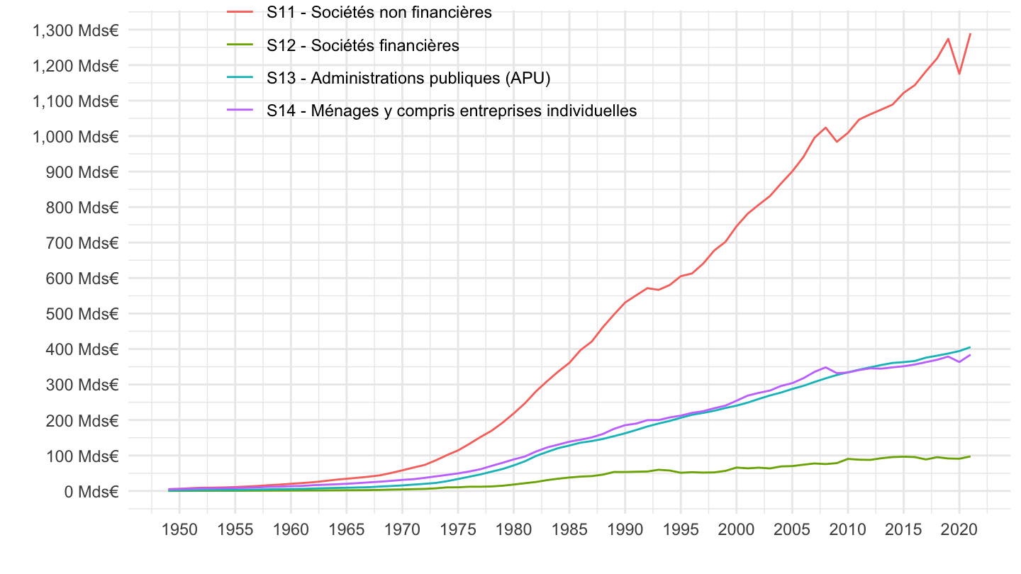
`CNA-2014-CSI` |>

  filter(`SECT-INST` %in% c("S11", "S12", "S14", "S13"),
         OPERATION %in% c("B1G")) |>
  year_to_date() |>
  left_join(gdp, by = "date") |>
  ggplot() + geom_line(aes(x = date, y = OBS_VALUE/gdp, color = `SECT-INST`)) +
  theme_minimal() +  xlab("") + ylab("") +

  scale_x_date(breaks = as.Date(paste0(seq(1940, 2100, 5), "-01-01")),
               labels = date_format("%Y")) +
  theme(legend.position = c(0.75, 0.6),
        legend.title = element_blank()) +
  scale_y_continuous(breaks = 0.01*seq(0, 2000, 5),
                     labels = percent_format(acc = 1))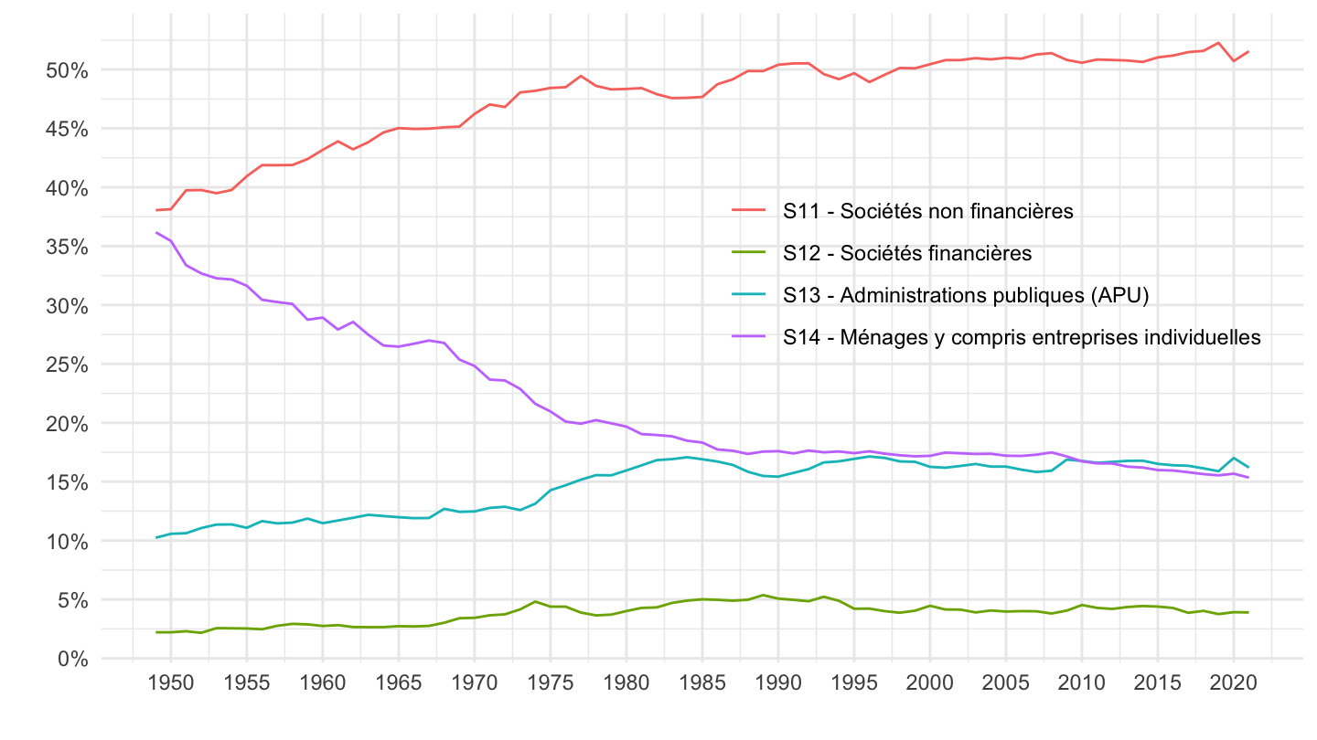
`CNA-2014-CSI` |>


  filter(`SECT-INST` %in% c("S0"),
         OPERATION %in% c("D41", "D42", "D43", "D44")) |>
  year_to_date() |>
  ggplot() + geom_line(aes(x = date, y = OBS_VALUE/1000, color = OPERATION)) +
  theme_minimal() +  xlab("") + ylab("") +

  scale_x_date(breaks = as.Date(paste0(seq(1940, 2100, 5), "-01-01")),
               labels = date_format("%Y")) +
  theme(legend.position = c(0.35, 0.9),
        legend.title = element_blank()) +
  scale_y_continuous(breaks = seq(0, 2000, 100),
                     labels = dollar_format(suffix = " Mds€", prefix = "", accuracy = 1))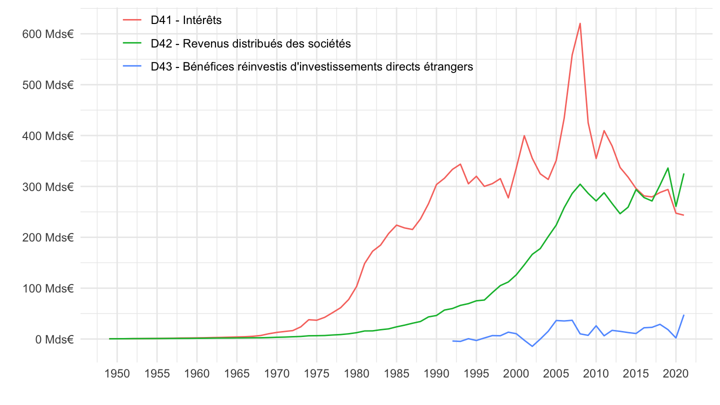
`CNA-2014-CSI` |>


  filter(`SECT-INST` %in% c("S0"),
         OPERATION %in% c("D41", "D42", "D43", "D44")) |>
  year_to_date() |>
  left_join(gdp, by = "date") |>
  ggplot() + geom_line(aes(x = date, y = OBS_VALUE/gdp, color = OPERATION)) +
  theme_minimal() +  xlab("") + ylab("") +

  scale_x_date(breaks = as.Date(paste0(seq(1940, 2100, 5), "-01-01")),
               labels = date_format("%Y")) +
  theme(legend.position = c(0.35, 0.9),
        legend.title = element_blank()) +
  scale_y_continuous(breaks = 0.01*seq(0, 2000, 5),
                     labels = percent_format(acc = 1))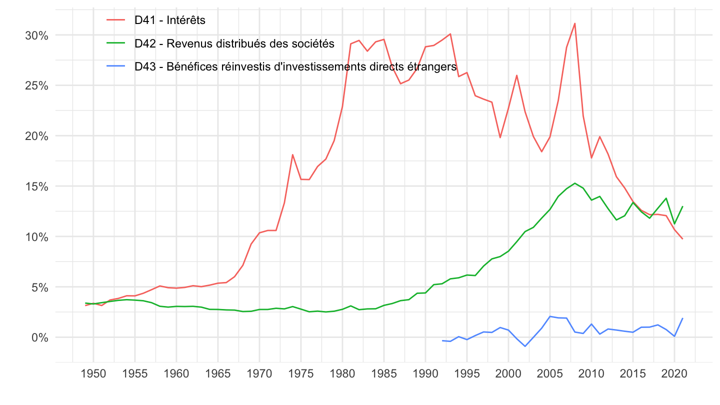
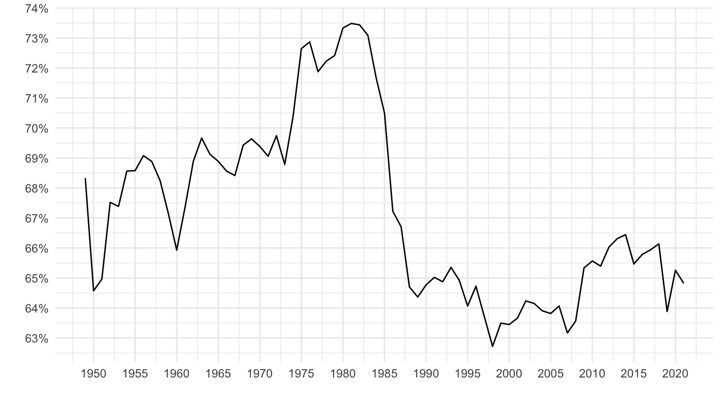
`CNA-2014-CSI` |>
  filter(`SECT-INST` == "S11",
         OPERATION %in% c("D1", "B1G"),
         NATURE == "SO",
         INDICATEUR == "CNA_COMPTES_SI_EA") |>
  year_to_date() |>
  select(date, OBS_VALUE, OPERATION) |>
  spread(OPERATION, OBS_VALUE) |>
  ggplot() + geom_line(aes(x = date, y = D1/B1G)) +
  theme_minimal() +  xlab("") + ylab("") +

  scale_x_date(breaks = as.Date(paste0(seq(1940, 2100, 5), "-01-01")),
               labels = date_format("%Y")) +
  theme(legend.position = c(0.35, 0.9),
        legend.title = element_blank()) +
  scale_y_continuous(breaks = 0.01*seq(-2, 90, 1),
                     labels = scales::percent_format(accuracy = 1))