Consommation des ménages en biens
Données - INSEE
Info
Last observation: 2026-05
First observation: 1980-01
Number of observations: 8 912
Last data update: 23 jul 2026, 22:47. Last compile: 24 jul 2026, 05:44
Structure
Données sur la macroéconomie en France
| source | dataset | Title | .html | .rData |
|---|---|---|---|---|
| bdf | CFT | Comptes Financiers Trimestriels | 2026-07-23 | 2025-03-09 |
| insee | CNA-2014-CONSO-SI | Dépenses de consommation finale par secteur institutionnel | 2026-07-23 | 2026-07-23 |
| insee | CNA-2014-CSI | Comptes des secteurs institutionnels | 2026-07-23 | 2026-07-23 |
| insee | CNA-2014-FBCF-BRANCHE | Formation brute de capital fixe (FBCF) par branche | 2026-07-23 | 2026-07-23 |
| insee | CNA-2014-FBCF-SI | Formation brute de capital fixe (FBCF) par secteur institutionnel | 2026-07-23 | 2026-07-23 |
| insee | CNA-2014-RDB | Revenu et pouvoir d’achat des ménages | 2026-07-23 | 2026-07-23 |
| insee | CNA-2020-CONSO-MEN | Consommation des ménages | 2026-07-23 | 2026-07-23 |
| insee | CNA-2020-PIB | Produit intérieur brut (PIB) et ses composantes | 2026-07-23 | 2026-07-23 |
| insee | CNT-2014-CB | Comptes des branches | 2026-07-23 | 2026-07-23 |
| insee | CNT-2014-CSI | Comptes de secteurs institutionnels | 2026-07-23 | 2026-07-22 |
| insee | CNT-2014-OPERATIONS | Opérations sur biens et services | 2026-07-23 | 2026-07-23 |
| insee | CNT-2014-PIB-EQB-RF | Équilibre du produit intérieur brut | 2026-07-23 | 2026-07-23 |
| insee | CONSO-MENAGES-2020 | Consommation des ménages en biens | 2026-07-23 | 2026-07-23 |
| insee | ICA-2015-IND-CONS | Indices de chiffre d'affaires dans l'industrie et la construction | 2026-07-23 | 2026-07-23 |
| insee | conso-mensuelle | Consommation de biens, données mensuelles | 2026-07-23 | 2023-07-04 |
| insee | t_1101 | 1.101 – Le produit intérieur brut et ses composantes à prix courants (En milliards d'euros) | 2026-07-23 | 2022-01-02 |
| insee | t_1102 | 1.102 – Le produit intérieur brut et ses composantes en volume aux prix de l'année précédente chaînés (En milliards d'euros 2014) | 2026-07-23 | 2020-10-30 |
| insee | t_1105 | 1.105 – Produit intérieur brut - les trois approches à prix courants (En milliards d'euros) - t_1105 | 2026-07-23 | 2020-10-30 |
Source
- s1036 - Consommation des ménages (base 2014). html
Table
Exemple
Code
`CONSO-MENAGES-2020` %>%
  filter(TIME_PERIOD %in% c("1980-01", "2000-01", "2020-01")) %>%

  select_if(function(col) length(unique(col)) > 1) %>%
  select(-IDBANK, -TITLE_FR, -TITLE_EN) %>%
  spread(TIME_PERIOD, OBS_VALUE) %>%
  arrange(-`2020-01`) %>%
print_table_conditional()| PRODUIT_CONSO_MENAGES | OBS_REV | Produit_conso_menages | 1980-01 | 2000-01 | 2020-01 |
|---|---|---|---|---|---|
| BIENS | 1 | Biens | NA | 38.012 | 47.927 |
| BIENS-MANUFACTURES | 1 | Biens manufacturés | NA | 31.251 | 40.561 |
| BIENS-FABRIQUES | 1 | Biens fabriqués | NA | NA | 21.297 |
| ALIMENTAIRE | 1 | Alimentaire | NA | NA | 18.015 |
| ALIMENTAIRE-HORS-TABAC | 1 | Alimentation hors tabac | NA | NA | 15.966 |
| BIENS-DURABLES | NA | Biens durables | 3.192 | 5.797 | 10.586 |
| ENERGIE_DEC2 | 1 | Énergie, eau, déchets, cokéfaction et raffinage (DE, C2) | NA | 9.007 | 8.575 |
| BIENS-FABRIQUES-AUTRES | 1 | Autres biens fabriqués | NA | NA | 6.143 |
| MATERIELS-TRANSPORT | NA | Matériels de transport | 3.119 | 4.937 | 5.538 |
| PRODUITS-PETROLIERS | 1 | Produits pétroliers | NA | 5.783 | 4.956 |
| TEXTILE | NA | Textile-cuir | 4.031 | 4.075 | 4.563 |
| ENERGIE_DE | 1 | Énergie, eau et déchets (DE) | NA | NA | 4.517 |
| ENERGIE_C2 | 1 | Cokéfaction et raffinage (C2) | NA | 4.572 | 3.994 |
| EQUIPEMENT-LOGEMENT | NA | Équipement du logement | 0.375 | 0.925 | 3.613 |
| ENERGIE_PETROLE | 1 | Énergie hors produits pétroliers | NA | NA | 3.558 |
| BIENS-DURABLES-EQUIPEMENT | NA | Biens durables d'équipement personnel | 0.745 | 1.066 | 1.440 |
| ALIMENTAIRE | NA | Alimentaire | 12.273 | 16.242 | NA |
| ALIMENTAIRE-HORS-TABAC | NA | Alimentation hors tabac | 9.830 | 13.280 | NA |
| BIENS | NA | Biens | 27.167 | NA | NA |
| BIENS-FABRIQUES | NA | Biens fabriqués | 9.491 | 13.889 | NA |
| BIENS-FABRIQUES-AUTRES | NA | Autres biens fabriqués | 2.852 | 4.246 | NA |
| BIENS-MANUFACTURES | NA | Biens manufacturés | 22.693 | NA | NA |
| ENERGIE_C2 | NA | Cokéfaction et raffinage (C2) | 4.134 | NA | NA |
| ENERGIE_DE | NA | Énergie, eau et déchets (DE) | 2.403 | 4.295 | NA |
| ENERGIE_DEC2 | NA | Énergie, eau, déchets, cokéfaction et raffinage (DE, C2) | 6.556 | NA | NA |
| ENERGIE_PETROLE | NA | Énergie hors produits pétroliers | 1.685 | 3.084 | NA |
| PRODUITS-PETROLIERS | NA | Produits pétroliers | 4.818 | NA | NA |
Total, Alimentaire, Alimentaire XTabac
All
Indice
Nouvelle version
Code
`CONSO-MENAGES-2020` %>%
  filter(PRODUIT_CONSO_MENAGES %in% c("BIENS", "ALIMENTAIRE", "ALIMENTAIRE-HORS-TABAC")) %>%

  month_to_date %>%
  group_by(Produit_conso_menages) %>%
  arrange(date) %>%
  mutate(OBS_VALUE = 100*OBS_VALUE/OBS_VALUE[1]) %>%
  ggplot + geom_line(aes(x = date, y = OBS_VALUE, color = Produit_conso_menages)) +
  theme_minimal() + ylab("Consommation mensuelle") + xlab("") +
  theme(legend.title = element_blank(),
        legend.position = c(0.2, 0.9)) +
  scale_x_date(breaks = seq(1950, 2030, 5) %>% paste0("-01-01") %>% as.Date,
               labels = date_format("%Y")) +
  scale_y_log10(breaks = seq(100, 300, 10))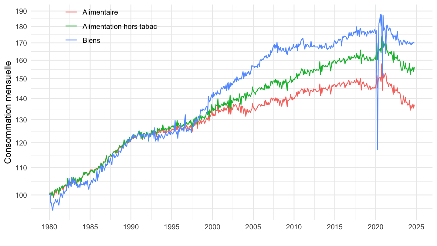
Comparer version
Code
`CONSO-MENAGES-2020` %>%
  mutate(methode = "Méthode 2020") %>%
  bind_rows(`CONSO-MENAGES-2014` %>%
              mutate(methode = "Méthode 2014, octobre 2023")) %>%
  bind_rows(`CONSO-MENAGES-2014-vieux` %>%
              mutate(methode = "Méthode 2014, septembre 2023")) %>%
  filter(PRODUIT_CONSO_MENAGES %in% c("BIENS", "ALIMENTAIRE-HORS-TABAC")) %>%

  month_to_date %>%
  group_by(Produit_conso_menages, methode) %>%
  arrange(date) %>%
  mutate(OBS_VALUE = 100*OBS_VALUE/OBS_VALUE[1]) %>%
  ggplot + geom_line(aes(x = date, y = OBS_VALUE, color = Produit_conso_menages, linetype = methode)) +
  theme_minimal() + ylab("Consommation mensuelle") + xlab("") +
  theme(legend.title = element_blank(),
        legend.position = c(0.2, 0.8)) +
  scale_x_date(breaks = seq(1950, 2030, 5) %>% paste0("-01-01") %>% as.Date,
               labels = date_format("%Y")) +
  scale_y_log10(breaks = seq(100, 300, 10))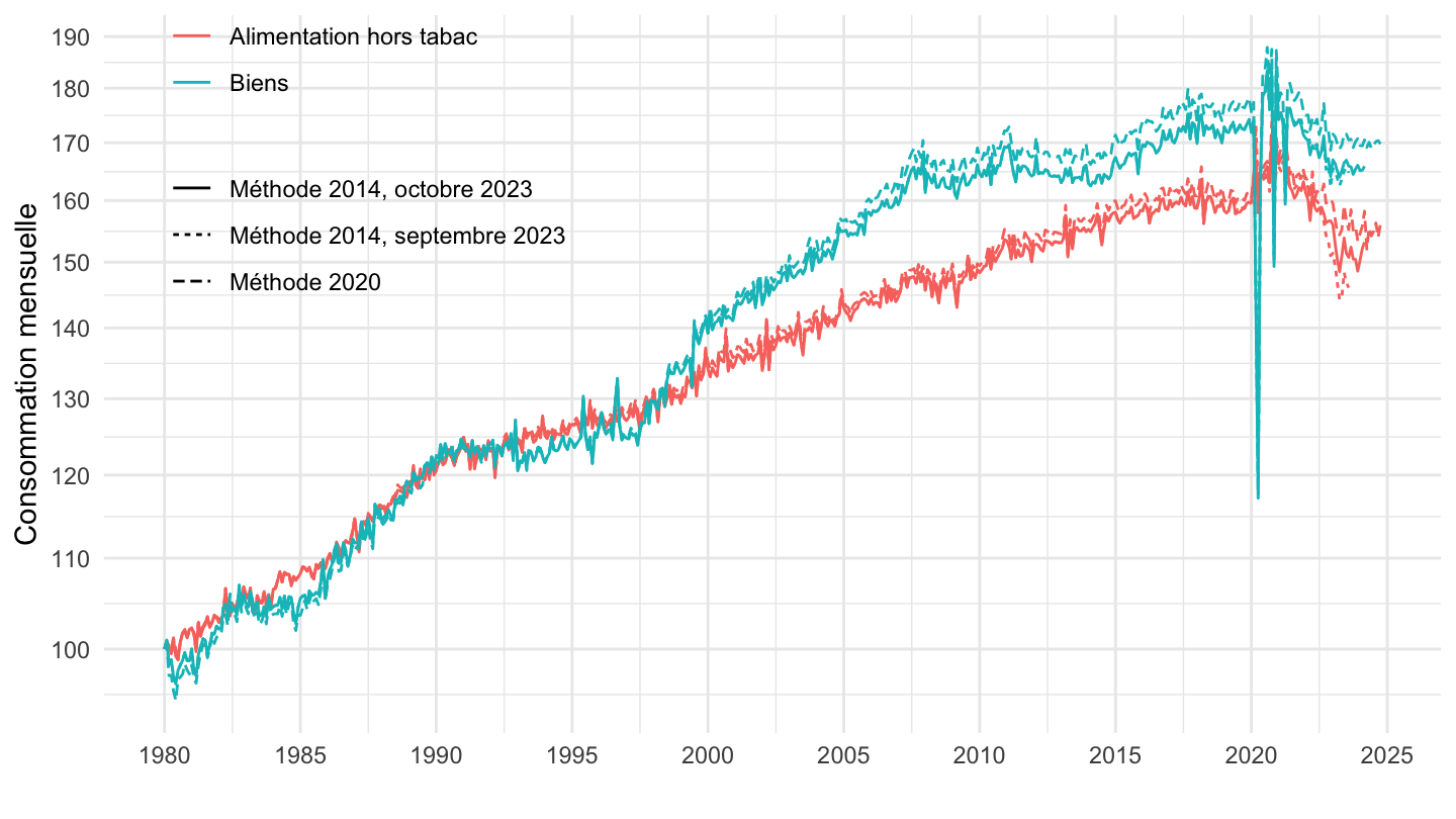
Baisse sur 6 mois
Code
Sys.setlocale("LC_TIME", "fr_CA.UTF-8")# [1] "fr_CA.UTF-8"Code
`CONSO-MENAGES-2020` %>%
  filter(PRODUIT_CONSO_MENAGES %in% c("ALIMENTAIRE", "ALIMENTAIRE-HORS-TABAC")) %>%

  month_to_date %>%
  arrange((date)) %>%
  group_by(Produit_conso_menages) %>%
  mutate(OBS_VALUE2 = OBS_VALUE/lag(OBS_VALUE, 6)-1) %>%
  ggplot + geom_line(aes(x = date, y = OBS_VALUE2, color = Produit_conso_menages)) +
  theme_minimal() + ylab("Evolution de la consommation sur 6 mois (%)") + xlab("") +
  theme(legend.title = element_blank(),
        legend.position = c(0.2, 0.3)) +
  scale_x_date(breaks = seq(1950, 2030, 5) %>% paste0("-01-01") %>% as.Date,
               labels = date_format("%Y")) +
  scale_y_continuous(breaks = 0.01*seq(-100, 500, 2),
                labels = percent_format(accuracy = 1))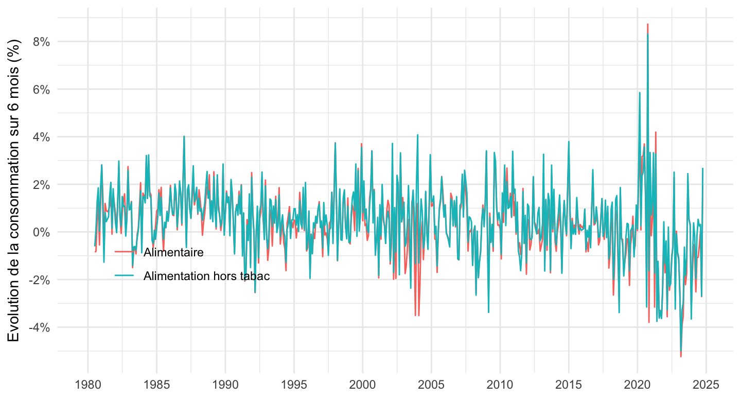
Baisse sur 12 mois
Code
Sys.setlocale("LC_TIME", "fr_CA.UTF-8")# [1] "fr_CA.UTF-8"Code
`CONSO-MENAGES-2020` %>%
  filter(PRODUIT_CONSO_MENAGES %in% c("ALIMENTAIRE", "ALIMENTAIRE-HORS-TABAC")) %>%

  month_to_date %>%
  arrange((date)) %>%
  group_by(Produit_conso_menages) %>%
  mutate(OBS_VALUE2 = OBS_VALUE/lag(OBS_VALUE, 12)-1) %>%
  ggplot + geom_line(aes(x = date, y = OBS_VALUE2, color = Produit_conso_menages)) +
  theme_minimal() + ylab("Evolution de la consommation sur 12 mois (%)") + xlab("") +
  theme(legend.title = element_blank(),
        legend.position = c(0.2, 0.3)) +
  scale_x_date(breaks = seq(1950, 2030, 5) %>% paste0("-01-01") %>% as.Date,
               labels = date_format("%Y")) +
  scale_y_continuous(breaks = 0.01*seq(-100, 500, 2),
                labels = percent_format(accuracy = 1))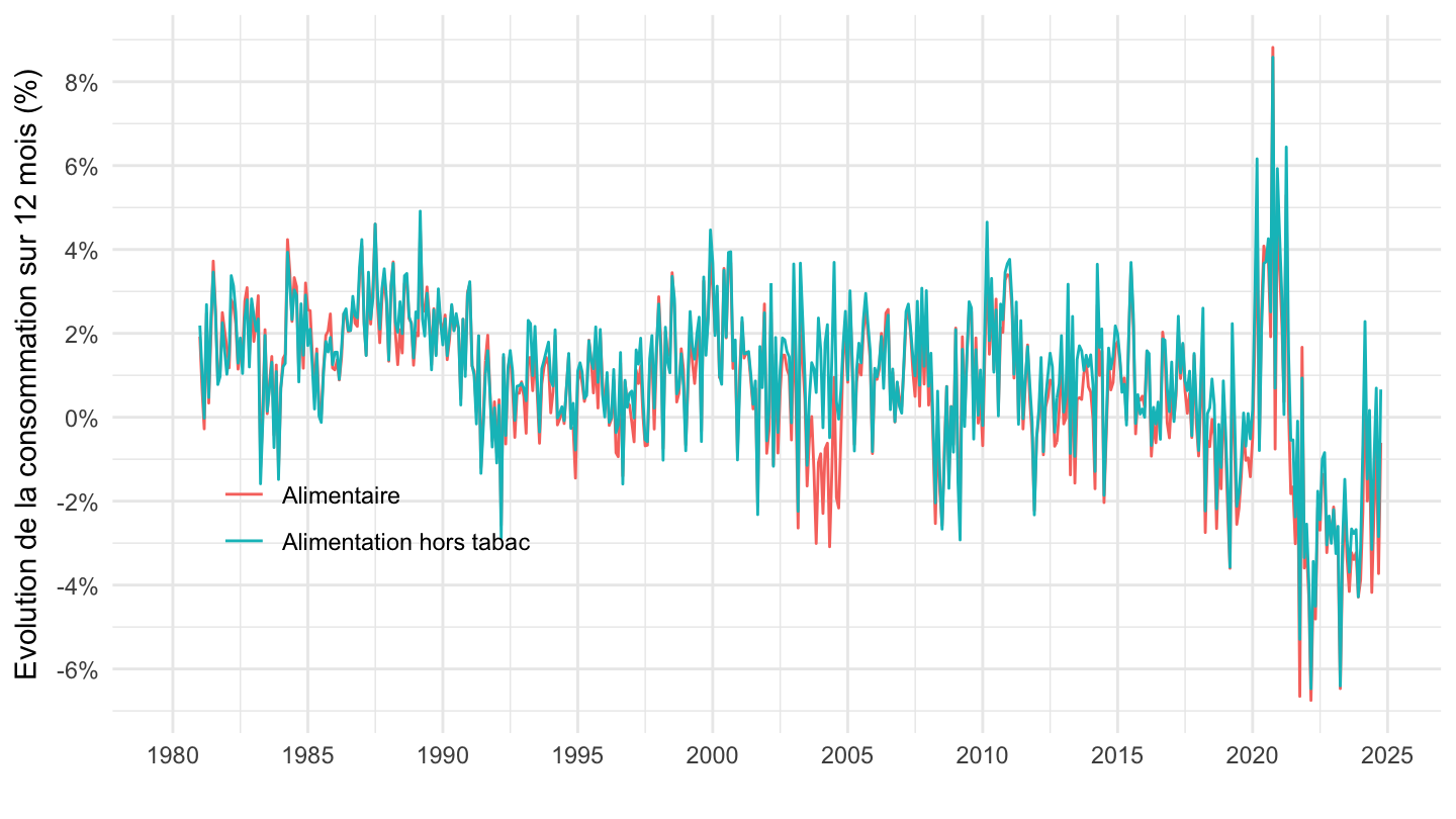
Baisse sur 18 mois
Code
Sys.setlocale("LC_TIME", "fr_CA.UTF-8")# [1] "fr_CA.UTF-8"Code
`CONSO-MENAGES-2020` %>%
  filter(PRODUIT_CONSO_MENAGES %in% c("ALIMENTAIRE", "ALIMENTAIRE-HORS-TABAC")) %>%

  month_to_date %>%
  arrange((date)) %>%
  group_by(Produit_conso_menages) %>%
  mutate(OBS_VALUE2 = OBS_VALUE/lag(OBS_VALUE, 18)-1) %>%
  arrange(desc(date)) %>%
  ggplot + geom_line(aes(x = date, y = OBS_VALUE2, color = Produit_conso_menages)) +
  theme_minimal() + ylab("Evolution de la consommation sur 18 mois (%)") + xlab("") +
  theme(legend.title = element_blank(),
        legend.position = c(0.2, 0.3)) +
  scale_x_date(breaks = seq(1950, 2030, 5) %>% paste0("-01-01") %>% as.Date,
               labels = date_format("%Y")) +
  scale_y_continuous(breaks = 0.01*seq(-100, 500, 2),
                labels = percent_format(accuracy = 1))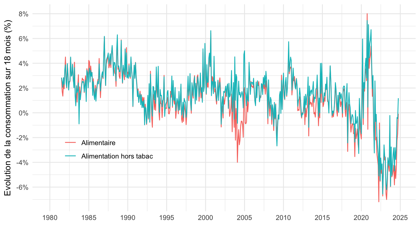
Baisse sur 24 mois
Code
Sys.setlocale("LC_TIME", "fr_CA.UTF-8")# [1] "fr_CA.UTF-8"Code
`CONSO-MENAGES-2020` %>%
  filter(PRODUIT_CONSO_MENAGES %in% c("ALIMENTAIRE", "ALIMENTAIRE-HORS-TABAC")) %>%

  month_to_date %>%
  arrange((date)) %>%
  group_by(Produit_conso_menages) %>%
  mutate(OBS_VALUE2 = OBS_VALUE/lag(OBS_VALUE, 24)-1) %>%
  ggplot + geom_line(aes(x = date, y = OBS_VALUE2, color = Produit_conso_menages)) +
  theme_minimal() + ylab("Evolution de la consommation sur 24 mois (%)") + xlab("") +
  theme(legend.title = element_blank(),
        legend.position = c(0.2, 0.3)) +
  scale_x_date(breaks = seq(1950, 2030, 5) %>% paste0("-01-01") %>% as.Date,
               labels = date_format("%Y")) +
  scale_y_continuous(breaks = 0.01*seq(-100, 500, 2),
                labels = percent_format(accuracy = 1))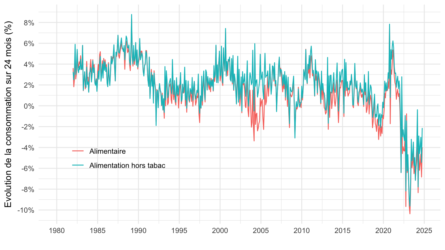
Baisse sur 36 mois
Code
Sys.setlocale("LC_TIME", "fr_CA.UTF-8")# [1] "fr_CA.UTF-8"Code
`CONSO-MENAGES-2020` %>%
  filter(PRODUIT_CONSO_MENAGES %in% c("ALIMENTAIRE", "ALIMENTAIRE-HORS-TABAC")) %>%

  month_to_date %>%
  arrange((date)) %>%
  group_by(Produit_conso_menages) %>%
  mutate(OBS_VALUE2 = OBS_VALUE/lag(OBS_VALUE, 36)-1) %>%
  ggplot + geom_line(aes(x = date, y = OBS_VALUE2, color = Produit_conso_menages)) +
  theme_minimal() + ylab("Evolution de la consommation sur 36 mois (%)") + xlab("") +
  theme(legend.title = element_blank(),
        legend.position = c(0.2, 0.3)) +
  scale_x_date(breaks = seq(1950, 2030, 5) %>% paste0("-01-01") %>% as.Date,
               labels = date_format("%Y")) +
  scale_y_continuous(breaks = 0.01*seq(-100, 500, 2),
                labels = percent_format(accuracy = 1))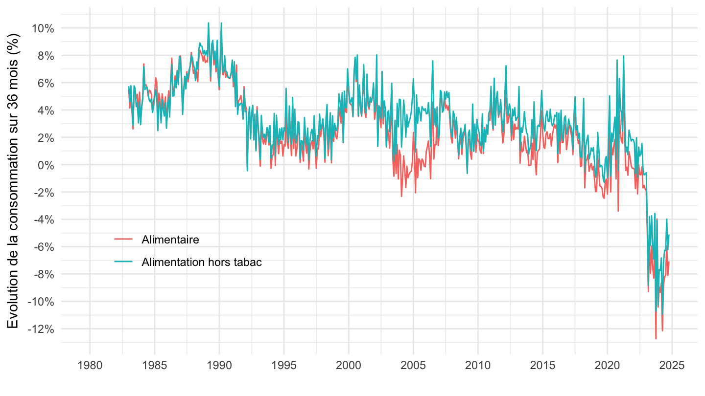
Baisse sur 48 mois
Code
Sys.setlocale("LC_TIME", "fr_CA.UTF-8")# [1] "fr_CA.UTF-8"Code
`CONSO-MENAGES-2020` %>%
  filter(PRODUIT_CONSO_MENAGES %in% c("ALIMENTAIRE", "ALIMENTAIRE-HORS-TABAC")) %>%

  month_to_date %>%
  arrange((date)) %>%
  group_by(Produit_conso_menages) %>%
  mutate(OBS_VALUE2 = OBS_VALUE/lag(OBS_VALUE, 48)-1) %>%
  ggplot + geom_line(aes(x = date, y = OBS_VALUE2, color = Produit_conso_menages)) +
  theme_minimal() + ylab("Evolution de la consommation sur 4 ans (%)") + xlab("") +
  theme(legend.title = element_blank(),
        legend.position = c(0.2, 0.3)) +
  scale_x_date(breaks = seq(1950, 2030, 5) %>% paste0("-01-01") %>% as.Date,
               labels = date_format("%Y")) +
  scale_y_continuous(breaks = 0.01*seq(-100, 500, 2),
                labels = percent_format(accuracy = 1))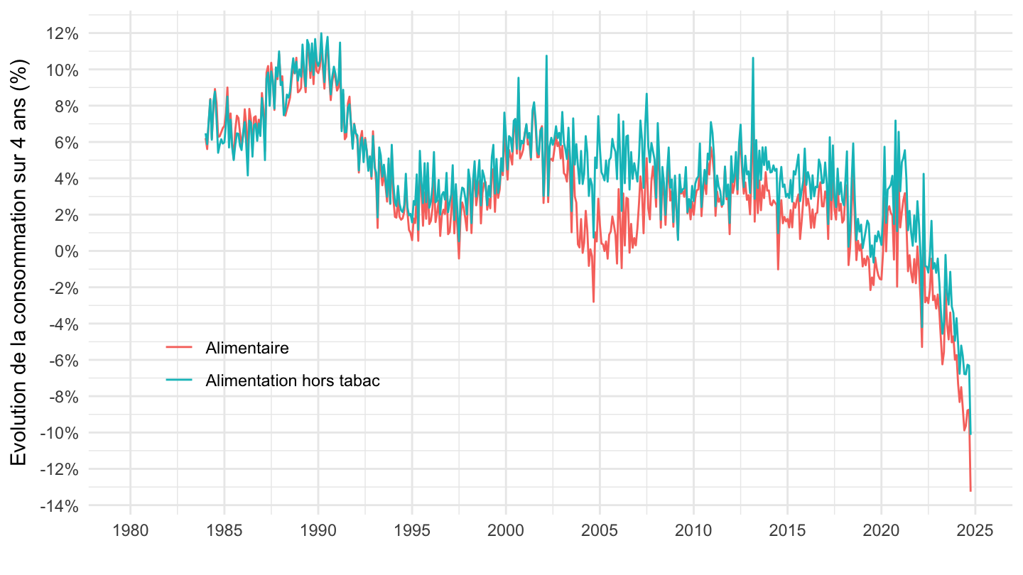
Tous
Code
`CONSO-MENAGES-2020` %>%
  filter(PRODUIT_CONSO_MENAGES %in% c("BIENS", "ALIMENTAIRE", "ALIMENTAIRE-HORS-TABAC")) %>%

  month_to_date %>%
  #filter(date >= as.Date("1996-01-01")) %>%
  group_by(Produit_conso_menages) %>%
  arrange(date) %>%
  mutate(OBS_VALUE = 100*OBS_VALUE/OBS_VALUE[1]) %>%
  ggplot + geom_line(aes(x = date, y = OBS_VALUE, color = Produit_conso_menages)) +
  theme_minimal() + ylab("Consommation mensuelle") + xlab("") +
  theme(legend.title = element_blank(),
        legend.position = c(0.2, 0.8)) +
  scale_x_date(breaks = seq(1950, 2030, 5) %>% paste0("-01-01") %>% as.Date,
               labels = date_format("%Y")) +
  scale_y_log10(breaks = seq(10, 300, 10))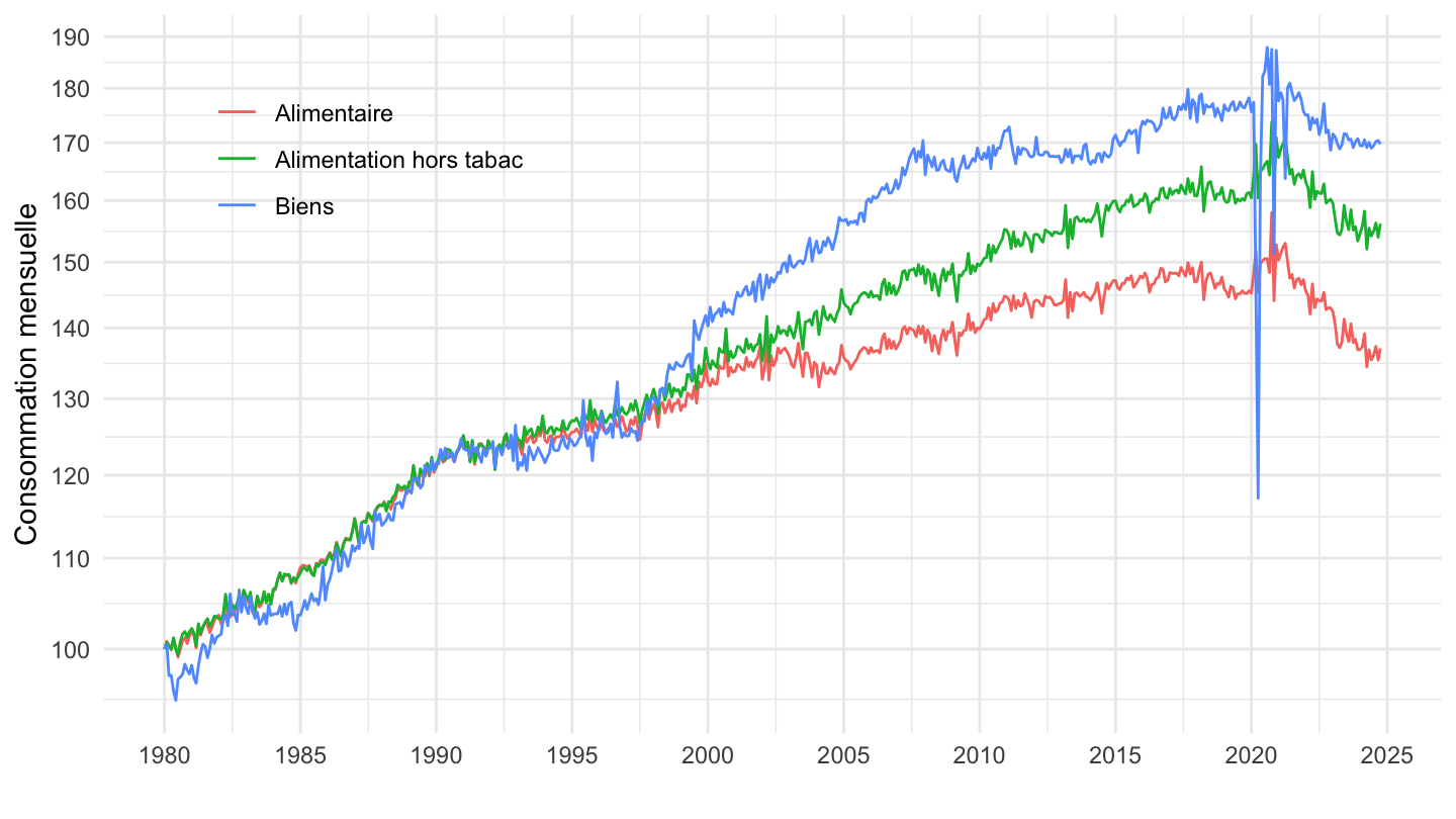
1996-
Code
`CONSO-MENAGES-2020` %>%
  filter(PRODUIT_CONSO_MENAGES %in% c("BIENS", "ALIMENTAIRE", "ALIMENTAIRE-HORS-TABAC")) %>%

  month_to_date %>%
  filter(date >= as.Date("1996-01-01")) %>%
  group_by(Produit_conso_menages) %>%
  arrange(date) %>%
  mutate(OBS_VALUE = 100*OBS_VALUE/OBS_VALUE[1]) %>%
  ggplot + geom_line(aes(x = date, y = OBS_VALUE, color = Produit_conso_menages)) +
  theme_minimal() + ylab("Consommation mensuelle") + xlab("") +
  theme(legend.title = element_blank(),
        legend.position = c(0.2, 0.8)) +
  scale_x_date(breaks = seq(1950, 2030, 2) %>% paste0("-01-01") %>% as.Date,
               labels = date_format("%Y")) +
  scale_y_log10(breaks = seq(10, 300, 10))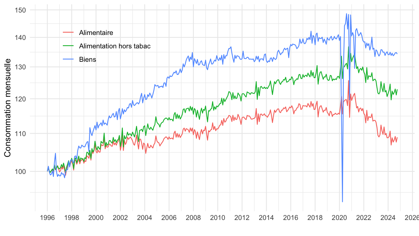
2002-
Code
`CONSO-MENAGES-2020` %>%
  filter(PRODUIT_CONSO_MENAGES %in% c("BIENS", "ALIMENTAIRE", "ALIMENTAIRE-HORS-TABAC")) %>%

  month_to_date %>%
  filter(date >= as.Date("2002-01-01")) %>%
  group_by(Produit_conso_menages) %>%
  arrange(date) %>%
  mutate(OBS_VALUE = 100*OBS_VALUE/OBS_VALUE[1]) %>%
  ggplot + geom_line(aes(x = date, y = OBS_VALUE, color = Produit_conso_menages)) +
  theme_minimal() + ylab("Consommation mensuelle") + xlab("") +
  theme(legend.title = element_blank(),
        legend.position = c(0.2, 0.9)) +
  scale_x_date(breaks = seq(1950, 2030, 2) %>% paste0("-01-01") %>% as.Date,
               labels = date_format("%Y")) +
  scale_y_log10(breaks = seq(10, 300, 10))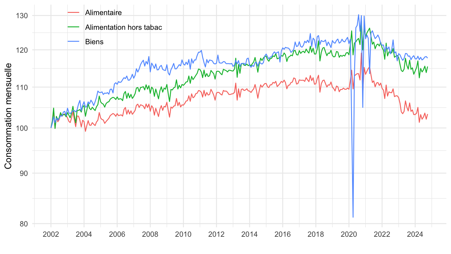
2005-
Code
`CONSO-MENAGES-2020` %>%
  filter(PRODUIT_CONSO_MENAGES %in% c("BIENS", "ALIMENTAIRE", "ALIMENTAIRE-HORS-TABAC")) %>%

  month_to_date %>%
  filter(date >= as.Date("2005-01-01")) %>%
  group_by(Produit_conso_menages) %>%
  arrange(date) %>%
  mutate(OBS_VALUE = 100*OBS_VALUE/OBS_VALUE[1]) %>%
  ggplot + geom_line(aes(x = date, y = OBS_VALUE, color = Produit_conso_menages)) +
  theme_minimal() + ylab("Consommation mensuelle") + xlab("") +
  theme(legend.title = element_blank(),
        legend.position = c(0.2, 0.3)) +
  scale_x_date(breaks = seq(1950, 2030, 2) %>% paste0("-01-01") %>% as.Date,
               labels = date_format("%Y")) +
  scale_y_log10(breaks = seq(10, 300, 10))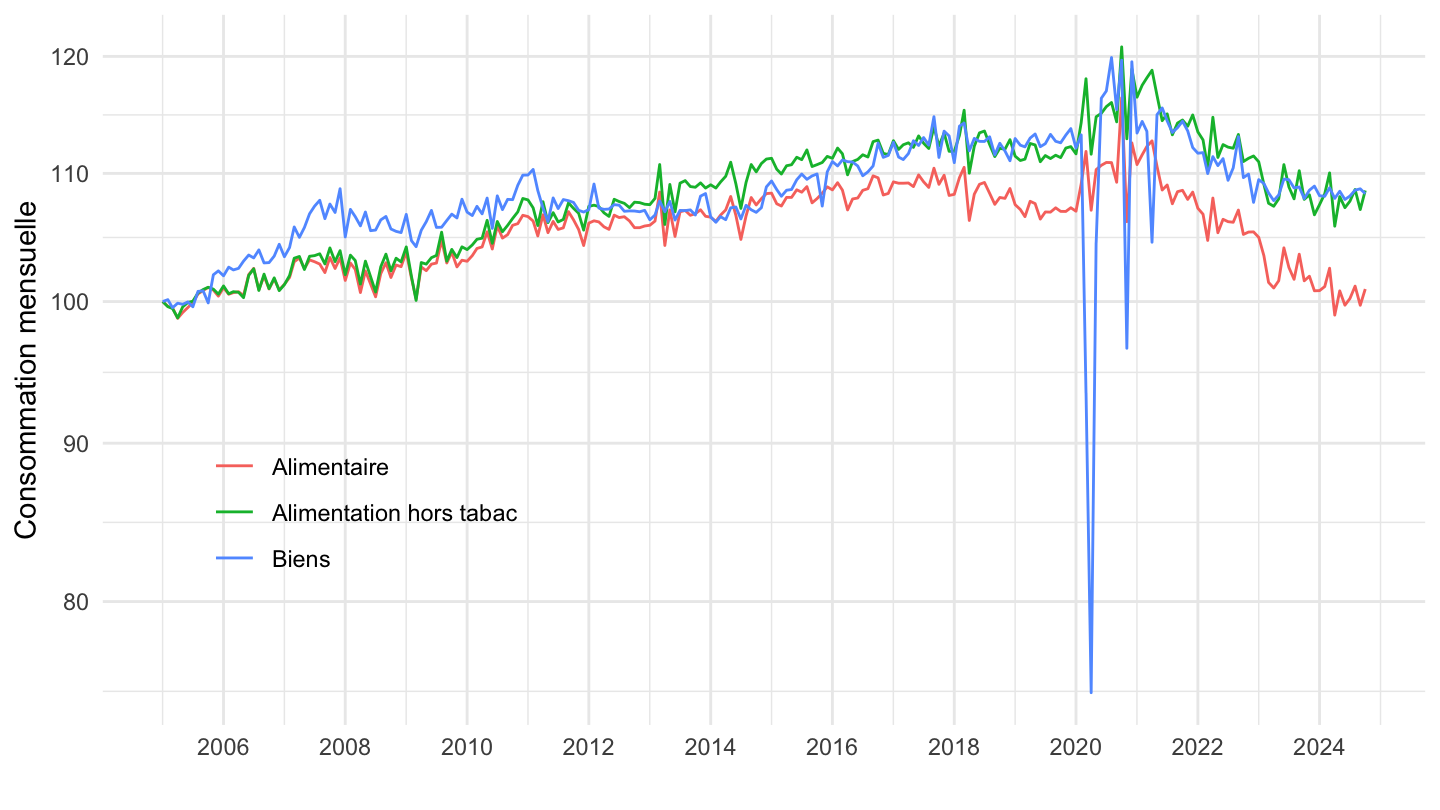
2010-
Code
`CONSO-MENAGES-2020` %>%
  filter(PRODUIT_CONSO_MENAGES %in% c("BIENS", "ALIMENTAIRE", "ALIMENTAIRE-HORS-TABAC")) %>%

  month_to_date %>%
  filter(date >= as.Date("2010-01-01")) %>%
  group_by(Produit_conso_menages) %>%
  arrange(date) %>%
  mutate(OBS_VALUE = 100*OBS_VALUE/OBS_VALUE[1]) %>%
  ggplot + geom_line(aes(x = date, y = OBS_VALUE, color = Produit_conso_menages)) +
  theme_minimal() + ylab("Consommation mensuelle") + xlab("") +
  theme(legend.title = element_blank(),
        legend.position = c(0.2, 0.3)) +
  scale_x_date(breaks = seq(1950, 2030, 1) %>% paste0("-01-01") %>% as.Date,
               labels = date_format("%Y")) +
  scale_y_log10(breaks = seq(10, 300, 5))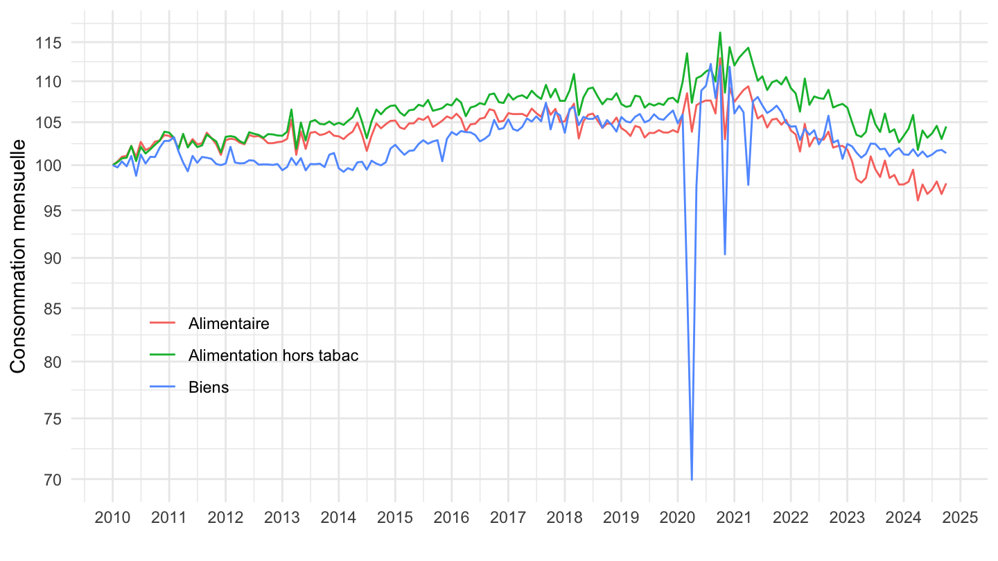
2017-
Code
`CONSO-MENAGES-2020` %>%
  filter(PRODUIT_CONSO_MENAGES %in% c("BIENS", "ALIMENTAIRE", "ALIMENTAIRE-HORS-TABAC")) %>%

  month_to_date %>%
  filter(date >= as.Date("2017-01-01")) %>%
  group_by(Produit_conso_menages) %>%
  arrange(date) %>%
  mutate(OBS_VALUE = 100*OBS_VALUE/OBS_VALUE[1]) %>%
  ggplot + geom_line(aes(x = date, y = OBS_VALUE, color = Produit_conso_menages)) +
  theme_minimal() + ylab("Consommation mensuelle") + xlab("") +
  theme(legend.title = element_blank(),
        legend.position = c(0.2, 0.3)) +
  scale_x_date(breaks = seq(1950, 2030, 1) %>% paste0("-01-01") %>% as.Date,
               labels = date_format("%Y")) +
  scale_y_log10(breaks = seq(10, 300, 5))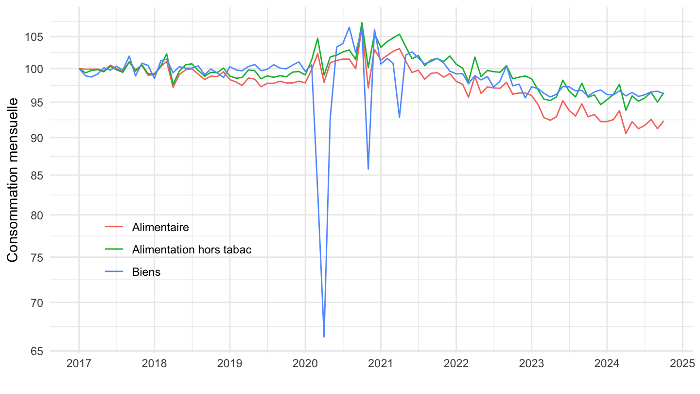
2010
Comparer version
Code
Sys.setlocale("LC_TIME", "fr_CA.UTF-8")# [1] "fr_CA.UTF-8"Code
`CONSO-MENAGES-2020` %>%
  mutate(methode = "Méthode 2020") %>%
  bind_rows(`CONSO-MENAGES-2014` %>%
              mutate(methode = "Méthode 2014, 10/2023")) %>%
  bind_rows(`CONSO-MENAGES-2014-vieux` %>%
              mutate(methode = "Méthode 2014, 09/2023")) %>%
  filter(PRODUIT_CONSO_MENAGES %in% c("ALIMENTAIRE","ALIMENTAIRE-HORS-TABAC")) %>%

  month_to_date %>%
  filter(date >= as.Date("2010-01-01")) %>%
  group_by(Produit_conso_menages, methode) %>%
  arrange(date) %>%
  mutate(OBS_VALUE = 100*OBS_VALUE/OBS_VALUE[1]) %>%
  select(date, OBS_VALUE, Produit_conso_menages, methode) %>%
  ggplot + geom_line(aes(x = date, y = OBS_VALUE, color = Produit_conso_menages, linetype = methode)) +
  theme_minimal() + ylab("Consommation mensuelle (vs Janvier 2010)") + xlab("") +
  theme(legend.title = element_blank(),
               axis.text.x = element_text(angle = 45, vjust = 1, hjust = 1),
        legend.position = c(0.2, 0.8)) +
  scale_x_date(breaks = "6 months",
               labels = date_format("%B %Y")) +
  scale_y_log10(breaks = seq(10, 300, 1),
                labels = percent(seq(10, 300, 1)/100-1, acc = 1)) +
  geom_hline(yintercept = 100, linetype = "dashed")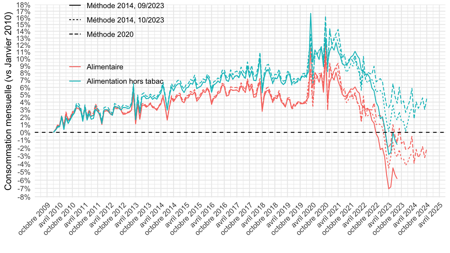
Janvier 2018-
Comparer version
Code
Sys.setlocale("LC_TIME", "fr_CA.UTF-8")# [1] "fr_CA.UTF-8"Code
`CONSO-MENAGES-2020` %>%
  mutate(methode = "Méthode 2020") %>%
  bind_rows(`CONSO-MENAGES-2014` %>%
              mutate(methode = "Méthode 2014, octobre 2023")) %>%
  bind_rows(`CONSO-MENAGES-2014-vieux` %>%
              mutate(methode = "Méthode 2014, septembre 2023")) %>%
  filter(PRODUIT_CONSO_MENAGES %in% c("ALIMENTAIRE","ALIMENTAIRE-HORS-TABAC")) %>%

  month_to_date %>%
  filter(date >= as.Date("2018-01-01")) %>%
  group_by(Produit_conso_menages, methode) %>%
  arrange(date) %>%
  mutate(OBS_VALUE = 100*OBS_VALUE/OBS_VALUE[1]) %>%
  select(date, OBS_VALUE, Produit_conso_menages, methode) %>%
  ggplot + geom_line(aes(x = date, y = OBS_VALUE, color = Produit_conso_menages, linetype = methode)) +
  theme_minimal() + ylab("Consommation mensuelle (vs. Janvier 2018)") + xlab("") +
  theme(legend.title = element_blank(),
               axis.text.x = element_text(angle = 45, vjust = 1, hjust = 1),
        legend.position = c(0.2, 0.3)) +
  scale_x_date(breaks = "3 months",
               labels = date_format("%B %Y")) +
  scale_y_log10(breaks = seq(10, 300, 1),
                labels = percent(seq(10, 300, 1)/100-1, acc = 1)) +
  geom_hline(yintercept = 100, linetype = "dashed")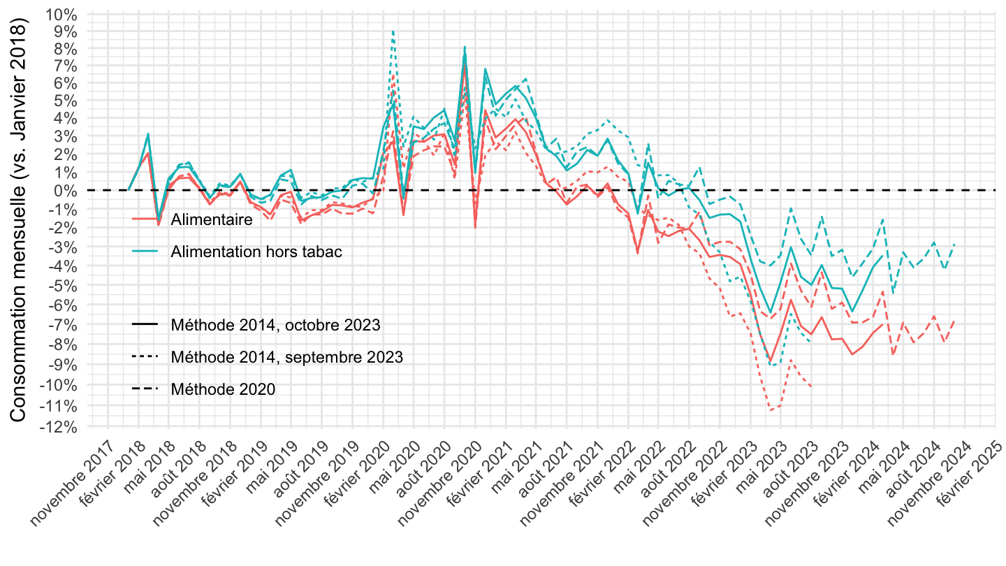
Mai 2020-
Code
Sys.setlocale("LC_TIME", "fr_CA.UTF-8")# [1] "fr_CA.UTF-8"Code
`CONSO-MENAGES-2020` %>%
  filter(PRODUIT_CONSO_MENAGES %in% c("BIENS", "ALIMENTAIRE", "ALIMENTAIRE-HORS-TABAC")) %>%

  month_to_date %>%
  filter(date >= as.Date("2020-05-01")) %>%
  group_by(Produit_conso_menages) %>%
  arrange(date) %>%
  mutate(OBS_VALUE = 100*OBS_VALUE/OBS_VALUE[1]) %>%
  ggplot + geom_line(aes(x = date, y = OBS_VALUE, color = Produit_conso_menages)) +
  theme_minimal() + ylab("Consommation mensuelle") + xlab("") +
  theme(legend.title = element_blank(),
               axis.text.x = element_text(angle = 45, vjust = 1, hjust = 1),
        legend.position = c(0.2, 0.15)) +
  scale_x_date(breaks = "3 months",
               labels = date_format("%b %Y")) +
  scale_y_log10(breaks = seq(10, 300, 5))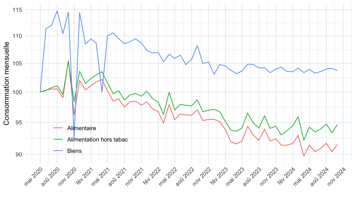
Janvier 2019-
Comparer version
Code
Sys.setlocale("LC_TIME", "fr_CA.UTF-8")# [1] "fr_CA.UTF-8"Code
`CONSO-MENAGES-2020` %>%
  mutate(methode = "Méthode 2020") %>%
  bind_rows(`CONSO-MENAGES-2014` %>%
              mutate(methode = "Méthode 2014, octobre 2023")) %>%
  bind_rows(`CONSO-MENAGES-2014-vieux` %>%
              mutate(methode = "Méthode 2014, septembre 2023")) %>%
  filter(PRODUIT_CONSO_MENAGES %in% c("ALIMENTAIRE","ALIMENTAIRE-HORS-TABAC")) %>%

  month_to_date %>%
  filter(date >= as.Date("2019-01-01")) %>%
  group_by(Produit_conso_menages, methode) %>%
  arrange(date) %>%
  mutate(OBS_VALUE = 100*OBS_VALUE/OBS_VALUE[1]) %>%
  select(date, OBS_VALUE, Produit_conso_menages, methode) %>%
  ggplot + geom_line(aes(x = date, y = OBS_VALUE, color = Produit_conso_menages, linetype = methode)) +
  theme_minimal() + ylab("Consommation mensuelle (Base 100 = Janvier 2019)") + xlab("") +
  theme(legend.title = element_blank(),
               axis.text.x = element_text(angle = 45, vjust = 1, hjust = 1),
        legend.position = c(0.2, 0.3)) +
  scale_x_date(breaks = "3 months",
               labels = date_format("%B %Y")) +
  scale_y_log10(breaks = seq(10, 300, 1),
                labels = percent(seq(10, 300, 1)/100-1, acc = 1))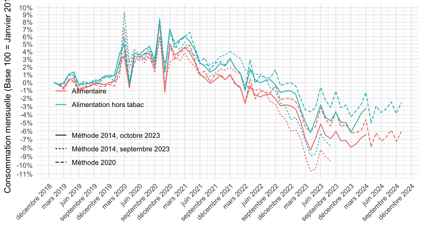
Janvier 2020-
Comparer version
Code
Sys.setlocale("LC_TIME", "fr_CA.UTF-8")# [1] "fr_CA.UTF-8"Code
`CONSO-MENAGES-2020` %>%
  mutate(methode = "Méthode 2020") %>%
  bind_rows(`CONSO-MENAGES-2014` %>%
              mutate(methode = "Méthode 2014, octobre 2023")) %>%
  bind_rows(`CONSO-MENAGES-2014-vieux` %>%
              mutate(methode = "Méthode 2014, septembre 2023")) %>%
  filter(PRODUIT_CONSO_MENAGES %in% c("ALIMENTAIRE","ALIMENTAIRE-HORS-TABAC")) %>%

  month_to_date %>%
  filter(date >= as.Date("2020-01-01")) %>%
  group_by(Produit_conso_menages, methode) %>%
  arrange(date) %>%
  mutate(OBS_VALUE = 100*OBS_VALUE/OBS_VALUE[1]) %>%
  select(date, OBS_VALUE, Produit_conso_menages, methode) %>%
  ggplot + geom_line(aes(x = date, y = OBS_VALUE, color = Produit_conso_menages, linetype = methode)) +
  theme_minimal() + ylab("Consommation mensuelle (Base 100 = Janvier 2020)") + xlab("") +
  theme(legend.title = element_blank(),
               axis.text.x = element_text(angle = 45, vjust = 1, hjust = 1),
        legend.position = c(0.2, 0.3)) +
  scale_x_date(breaks = "3 months",
               labels = date_format("%B %Y")) +
  scale_y_log10(breaks = seq(10, 300, 1),
                labels = percent(seq(10, 300, 1)/100-1, acc = 1))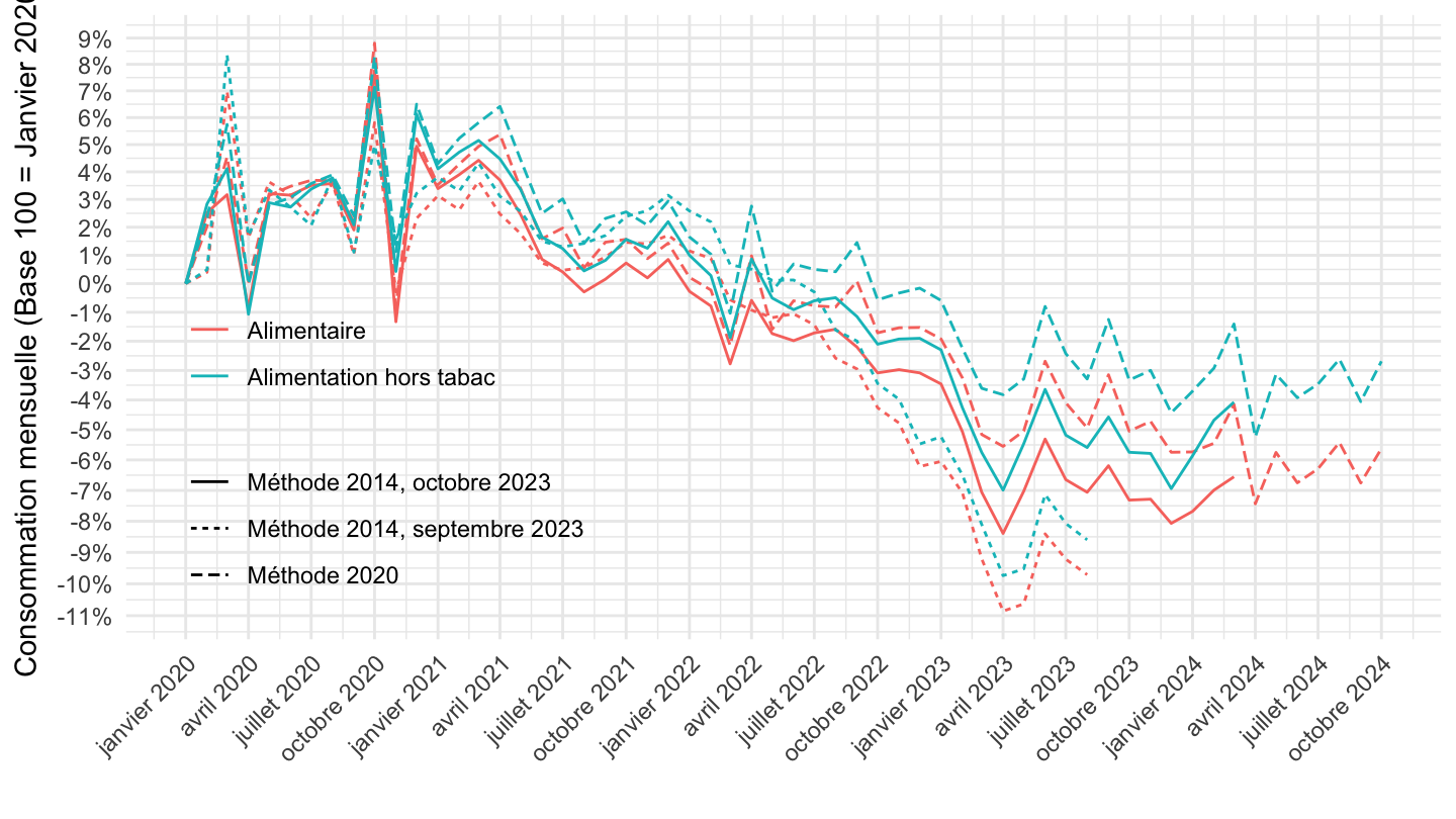
Janvier 2020 - Mai 2024
Comparer version
Code
Sys.setlocale("LC_TIME", "fr_CA.UTF-8")# [1] "fr_CA.UTF-8"Code
`CONSO-MENAGES-2020` %>%
  mutate(methode = "Méthode 2020") %>%
  bind_rows(`CONSO-MENAGES-2014` %>%
              mutate(methode = "Méthode 2014, octobre 2023")) %>%
  bind_rows(`CONSO-MENAGES-2014-vieux` %>%
              mutate(methode = "Méthode 2014, septembre 2023")) %>%
  filter(PRODUIT_CONSO_MENAGES %in% c("ALIMENTAIRE","ALIMENTAIRE-HORS-TABAC")) %>%

  month_to_date %>%
  filter(date >= as.Date("2020-01-01"),
         date <= as.Date("2024-05-01")) %>%
  group_by(Produit_conso_menages, methode) %>%
  arrange(date) %>%
  mutate(OBS_VALUE = 100*OBS_VALUE/OBS_VALUE[1]) %>%
  select(date, OBS_VALUE, Produit_conso_menages, methode) %>%
  mutate(methode = factor(methode, levels = c("Méthode 2014, septembre 2023",
                                             "Méthode 2014, octobre 2023",
                                             "Méthode 2020"))) %>%
  ggplot + geom_line(aes(x = date, y = OBS_VALUE, color = Produit_conso_menages, linetype = methode)) +
  theme_minimal() + ylab("Consommation mensuelle (Base 100 = Janvier 2020)") + xlab("") +
  theme(legend.title = element_blank(),
               axis.text.x = element_text(angle = 45, vjust = 1, hjust = 1),
        legend.position = c(0.2, 0.25)) +
  scale_x_date(breaks = "3 months",
               labels = date_format("%B %Y")) +
  scale_y_log10(breaks = seq(10, 300, 1),
                labels = percent(seq(10, 300, 1)/100-1, acc = 1))
Janvier 2022-
Nouvelle version
Code
Sys.setlocale("LC_TIME", "fr_CA.UTF-8")# [1] "fr_CA.UTF-8"Code
`CONSO-MENAGES-2020` %>%
  filter(PRODUIT_CONSO_MENAGES %in% c("BIENS", "ALIMENTAIRE")) %>%

  month_to_date %>%
  filter(date >= as.Date("2022-01-01")) %>%
  group_by(Produit_conso_menages) %>%
  arrange(date) %>%
  mutate(OBS_VALUE = 100*OBS_VALUE/OBS_VALUE[1]) %>%
  ggplot + geom_line(aes(x = date, y = OBS_VALUE, color = Produit_conso_menages)) +
  theme_minimal() + ylab("Consommation mensuelle\n(Base 100 = Janvier 2022)") + xlab("") +
  theme(legend.title = element_blank(),
               axis.text.x = element_text(angle = 45, vjust = 1, hjust = 1),
        legend.position = c(0.2, 0.2)) +
  scale_x_date(breaks = "2 months",
               labels = date_format("%B %Y")) +
  scale_y_log10(breaks = seq(10, 300, 1))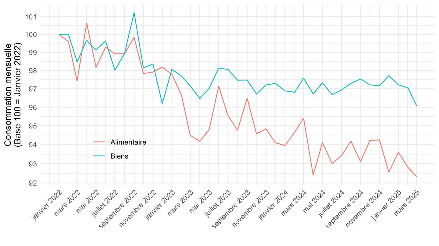
Décembre 2019-
Nouvelle version
Code
Sys.setlocale("LC_TIME", "fr_CA.UTF-8")# [1] "fr_CA.UTF-8"Code
`CONSO-MENAGES-2020` %>%
  filter(PRODUIT_CONSO_MENAGES %in% c("BIENS", "ALIMENTAIRE")) %>%

  month_to_date %>%
  filter(date >= as.Date("2019-12-01")) %>%
  group_by(Produit_conso_menages) %>%
  arrange(date) %>%
  mutate(OBS_VALUE = 100*OBS_VALUE/OBS_VALUE[1]) %>%
  mutate(OBS_VALUE = ifelse(year(date) == 2020 & month(date) %in% c(3, 4, 5, 10, 11), NA, OBS_VALUE)) %>%
  mutate(OBS_VALUE = ifelse(year(date) == 2021 & month(date) %in% c(3, 4), NA, OBS_VALUE)) %>%
  ggplot + geom_line(aes(x = date, y = OBS_VALUE, color = Produit_conso_menages)) +
  theme_minimal() + ylab("Consommation mensuelle\n(Base 100 = Décembre 2019)") + xlab("") +
  theme(legend.title = element_blank(),
               axis.text.x = element_text(angle = 45, vjust = 1, hjust = 1),
        legend.position = c(0.2, 0.2)) +
  scale_x_date(breaks = "2 months",
               labels = date_format("%B %Y")) +
  scale_y_log10(breaks = seq(10, 300, 1)) +
  geom_rect(data = data_frame(start = as.Date("2020-02-01"),
                                end = as.Date("2020-06-01")),
              aes(xmin = start, xmax = end, ymin = 0, ymax = +Inf), fill = viridis(4)[4], alpha = 0.2)+
  geom_rect(data = data_frame(start = as.Date("2020-09-01"),
                                end = as.Date("2020-12-01")),
              aes(xmin = start, xmax = end, ymin = 0, ymax = +Inf), fill = viridis(4)[4], alpha = 0.2)+
  geom_rect(data = data_frame(start = as.Date("2021-02-01"),
                                end = as.Date("2021-05-01")),
              aes(xmin = start, xmax = end, ymin = 0, ymax = +Inf), fill = viridis(4)[4], alpha = 0.2)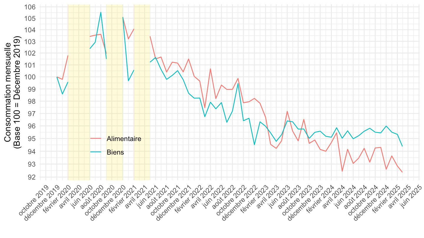
Juillet 2021-
Nouvelle version
Code
Sys.setlocale("LC_TIME", "fr_CA.UTF-8")# [1] "fr_CA.UTF-8"Code
`CONSO-MENAGES-2020` %>%
  filter(PRODUIT_CONSO_MENAGES %in% c("BIENS", "ALIMENTAIRE")) %>%

  month_to_date %>%
  filter(date >= as.Date("2021-07-01")) %>%
  group_by(Produit_conso_menages) %>%
  arrange(date) %>%
  mutate(OBS_VALUE = 100*OBS_VALUE/OBS_VALUE[1]) %>%
  ggplot + geom_line(aes(x = date, y = OBS_VALUE, color = Produit_conso_menages)) +
  theme_minimal() + ylab("Consommation mensuelle\n(Base 100 = Juillet 2021)") + xlab("") +
  theme(legend.title = element_blank(),
               axis.text.x = element_text(angle = 45, vjust = 1, hjust = 1),
        legend.position = c(0.2, 0.2)) +
  scale_x_date(breaks = "2 months",
               labels = date_format("%B %Y")) +
  scale_y_log10(breaks = seq(10, 300, 1))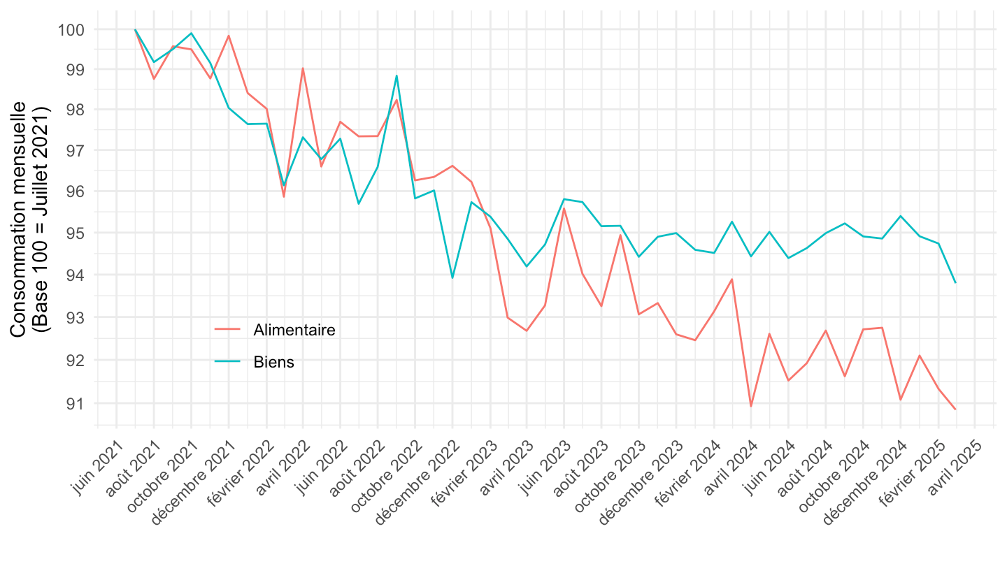
Comparer version
Code
Sys.setlocale("LC_TIME", "fr_CA.UTF-8")# [1] "fr_CA.UTF-8"Code
`CONSO-MENAGES-2020` %>%
  mutate(methode = "Méthode 2020") %>%
  bind_rows(`CONSO-MENAGES-2014` %>%
              mutate(methode = "Méthode 2014, octobre 2023")) %>%
  bind_rows(`CONSO-MENAGES-2014-vieux` %>%
              mutate(methode = "Méthode 2014, septembre 2023")) %>%
  filter(PRODUIT_CONSO_MENAGES %in% c("BIENS","ALIMENTAIRE-HORS-TABAC")) %>%

  month_to_date %>%
  filter(date >= as.Date("2021-07-01")) %>%
  group_by(Produit_conso_menages, methode) %>%
  arrange(date) %>%
  mutate(OBS_VALUE = 100*OBS_VALUE/OBS_VALUE[1]) %>%
  select(date, OBS_VALUE, Produit_conso_menages, methode) %>%
  ggplot + geom_line(aes(x = date, y = OBS_VALUE, color = Produit_conso_menages, linetype = methode)) +
  theme_minimal() + ylab("Consommation mensuelle (Base 100 = Février 2021)") + xlab("") +
  theme(legend.title = element_blank(),
               axis.text.x = element_text(angle = 45, vjust = 1, hjust = 1),
        legend.position = c(0.2, 0.3)) +
  scale_x_date(breaks = "1 month",
               labels = date_format("%B %Y")) +
  scale_y_log10(breaks = seq(10, 300, 1))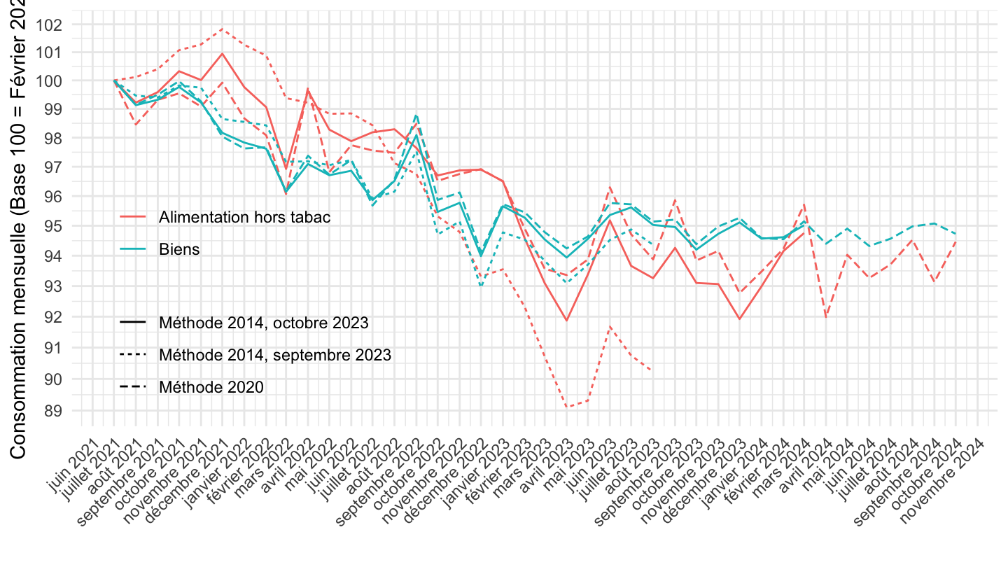
Dec 2021-
Nouvelle version
Code
Sys.setlocale("LC_TIME", "fr_CA.UTF-8")# [1] "fr_CA.UTF-8"Code
`CONSO-MENAGES-2020` %>%
  filter(PRODUIT_CONSO_MENAGES %in% c("BIENS", "ALIMENTAIRE", "ALIMENTAIRE-HORS-TABAC")) %>%

  month_to_date %>%
  filter(date >= as.Date("2021-12-01")) %>%
  group_by(Produit_conso_menages) %>%
  arrange(date) %>%
  mutate(OBS_VALUE = 100*OBS_VALUE/OBS_VALUE[1]) %>%
  ggplot + geom_line(aes(x = date, y = OBS_VALUE, color = Produit_conso_menages)) +
  theme_minimal() + ylab("Consommation mensuelle (Base 100 = Déc. 2021)") + xlab("") +
  theme(legend.title = element_blank(),
               axis.text.x = element_text(angle = 45, vjust = 1, hjust = 1),
        legend.position = c(0.2, 0.2)) +
  scale_x_date(breaks = "2 months",
               labels = date_format("%B %Y")) +
  scale_y_log10(breaks = seq(10, 300, 1))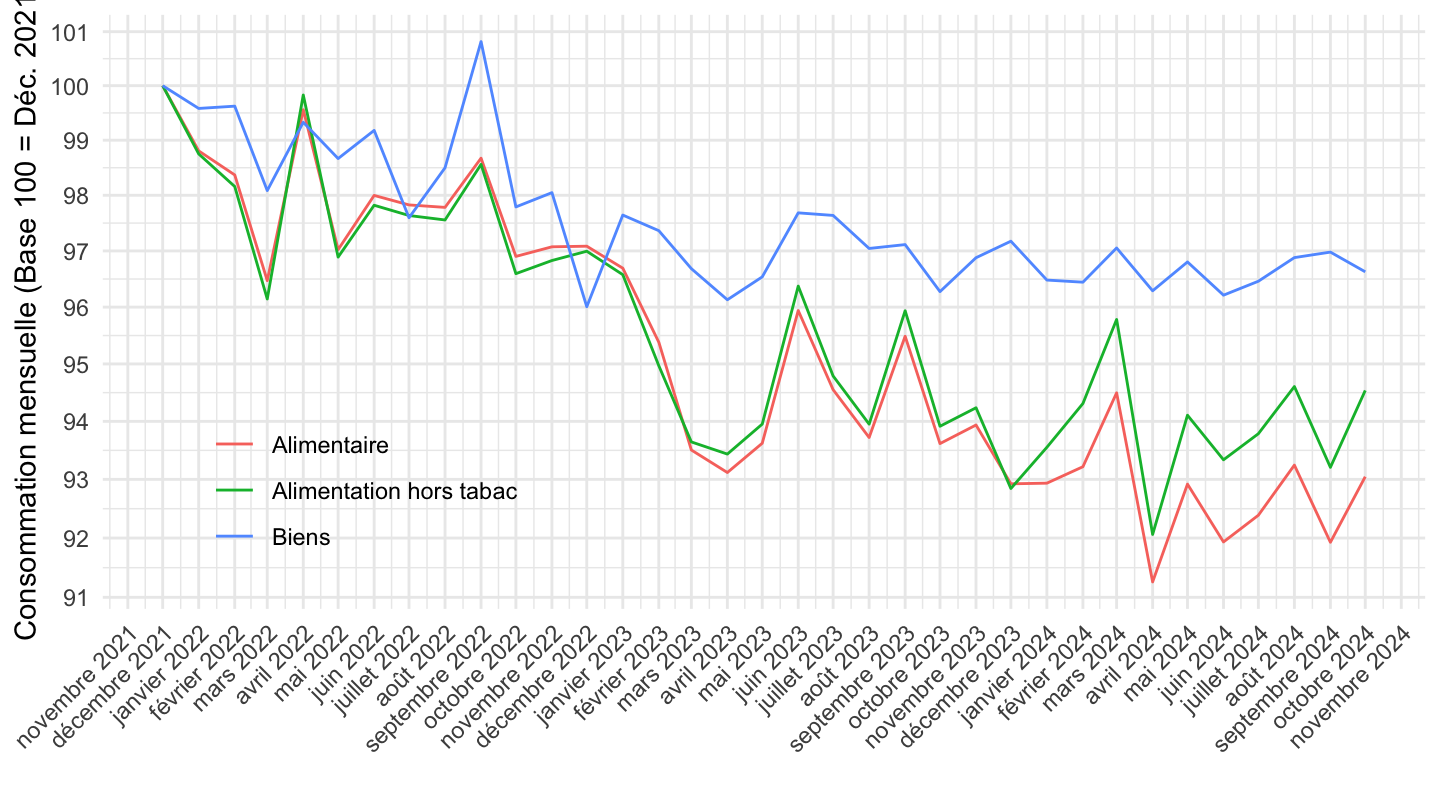
Comparer version
Code
Sys.setlocale("LC_TIME", "fr_CA.UTF-8")# [1] "fr_CA.UTF-8"Code
`CONSO-MENAGES-2020` %>%
  mutate(methode = "Base 2020") %>%
  bind_rows(`CONSO-MENAGES-2014` %>%
              mutate(methode = "Base 2014, méthode 10/2023")) %>%
  bind_rows(`CONSO-MENAGES-2014-vieux` %>%
              mutate(methode = "Base 2014, méthode 09/2023")) %>%
  filter(PRODUIT_CONSO_MENAGES %in% c("BIENS","ALIMENTAIRE-HORS-TABAC")) %>%

  month_to_date %>%
  filter(date >= as.Date("2021-12-01")) %>%
  group_by(Produit_conso_menages, methode) %>%
  arrange(date) %>%
  mutate(OBS_VALUE = 100*OBS_VALUE/OBS_VALUE[1]) %>%
  ggplot + geom_line(aes(x = date, y = OBS_VALUE, color = Produit_conso_menages, linetype = methode)) +
  theme_minimal() + ylab("Consommation mensuelle (Base 100 = Déc. 2021)") + xlab("") +
  theme(legend.title = element_blank(),
               axis.text.x = element_text(angle = 45, vjust = 1, hjust = 1),
        legend.position = c(0.2, 0.3)) +
  scale_x_date(breaks = "1 month",
               labels = date_format("%B %Y")) +
  scale_y_log10(breaks = seq(10, 300, 1))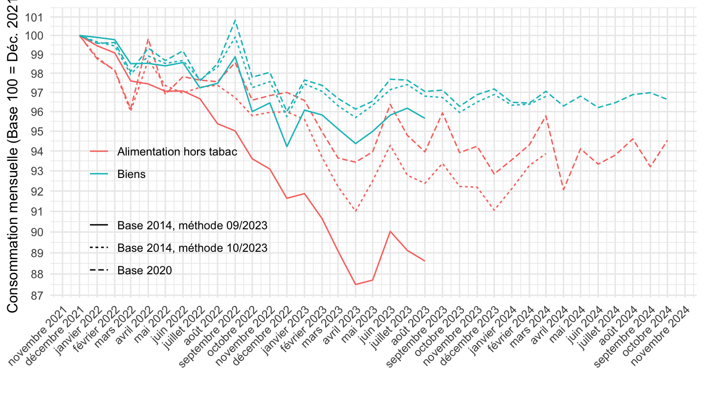
Comparer version
Code
Sys.setlocale("LC_TIME", "fr_CA.UTF-8")# [1] "fr_CA.UTF-8"Code
`CONSO-MENAGES-2020` %>%
  mutate(methode = "Base 2020") %>%
  bind_rows(`CONSO-MENAGES-2014` %>%
              mutate(methode = "Base 2014, méthode 10/2023")) %>%
  bind_rows(`CONSO-MENAGES-2014-vieux` %>%
              mutate(methode = "Base 2014, méthode 09/2023")) %>%
  filter(PRODUIT_CONSO_MENAGES %in% c("ALIMENTAIRE-HORS-TABAC")) %>%

  month_to_date %>%
  filter(date >= as.Date("2021-12-01")) %>%
  group_by(Produit_conso_menages, methode) %>%
  arrange(date) %>%
  mutate(OBS_VALUE = 100*OBS_VALUE/OBS_VALUE[1]) %>%
  ggplot + geom_line(aes(x = date, y = OBS_VALUE, color = methode)) +
  theme_minimal() + ylab("Consommation mensuelle (Base 100 = Déc. 2021)") + xlab("") +
  theme(legend.title = element_blank(),
               axis.text.x = element_text(angle = 45, vjust = 1, hjust = 1),
        legend.position = c(0.2, 0.3)) +
  scale_x_date(breaks = "1 month",
               labels = date_format("%B %Y")) +
  scale_y_log10(breaks = seq(10, 300, 1)) +
  geom_label(data = . %>% filter(date %in% c(as.Date("2023-08-01"))),
                                 aes(x = date, y = OBS_VALUE, label = percent(OBS_VALUE/100-1, acc = 0.1), color = methode))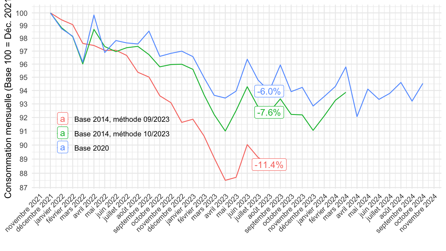
Février 2022-
Comparer version
Code
Sys.setlocale("LC_TIME", "fr_CA.UTF-8")# [1] "fr_CA.UTF-8"Code
`CONSO-MENAGES-2020` %>%
  mutate(methode = "Méthode 2020") %>%
  bind_rows(`CONSO-MENAGES-2014` %>%
              mutate(methode = "Méthode 2014, octobre 2023")) %>%
  bind_rows(`CONSO-MENAGES-2014-vieux` %>%
              mutate(methode = "Méthode 2014, septembre 2023")) %>%
  filter(PRODUIT_CONSO_MENAGES %in% c("BIENS","ALIMENTAIRE-HORS-TABAC")) %>%

  month_to_date %>%
  filter(date >= as.Date("2022-02-01")) %>%
  group_by(Produit_conso_menages, methode) %>%
  arrange(date) %>%
  mutate(OBS_VALUE = 100*OBS_VALUE/OBS_VALUE[1]) %>%
  select(date, OBS_VALUE, Produit_conso_menages, methode) %>%
  ggplot + geom_line(aes(x = date, y = OBS_VALUE, color = Produit_conso_menages, linetype = methode)) +
  theme_minimal() + ylab("Consommation mensuelle (Base 100 = Février 2021)") + xlab("") +
  theme(legend.title = element_blank(),
               axis.text.x = element_text(angle = 45, vjust = 1, hjust = 1),
        legend.position = c(0.2, 0.3)) +
  scale_x_date(breaks = "1 month",
               labels = date_format("%B %Y")) +
  scale_y_log10(breaks = seq(10, 300, 1))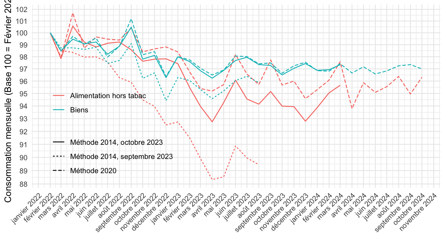
Total, Alimentaire
All
Code
`CONSO-MENAGES-2020` %>%
  filter(PRODUIT_CONSO_MENAGES %in% c("BIENS", "ALIMENTAIRE")) %>%

  month_to_date %>%
  group_by(Produit_conso_menages) %>%
  arrange(date) %>%
  mutate(OBS_VALUE = 100*OBS_VALUE/OBS_VALUE[1]) %>%
  ggplot + geom_line(aes(x = date, y = OBS_VALUE, color = Produit_conso_menages)) +
  theme_minimal() + ylab("Consommation mensuelle") + xlab("") +
  theme(legend.title = element_blank(),
        legend.position = c(0.2, 0.9)) +
  scale_x_date(breaks = seq(1950, 2030, 5) %>% paste0("-01-01") %>% as.Date,
               labels = date_format("%Y")) +
  scale_y_log10(breaks = seq(100, 300, 10))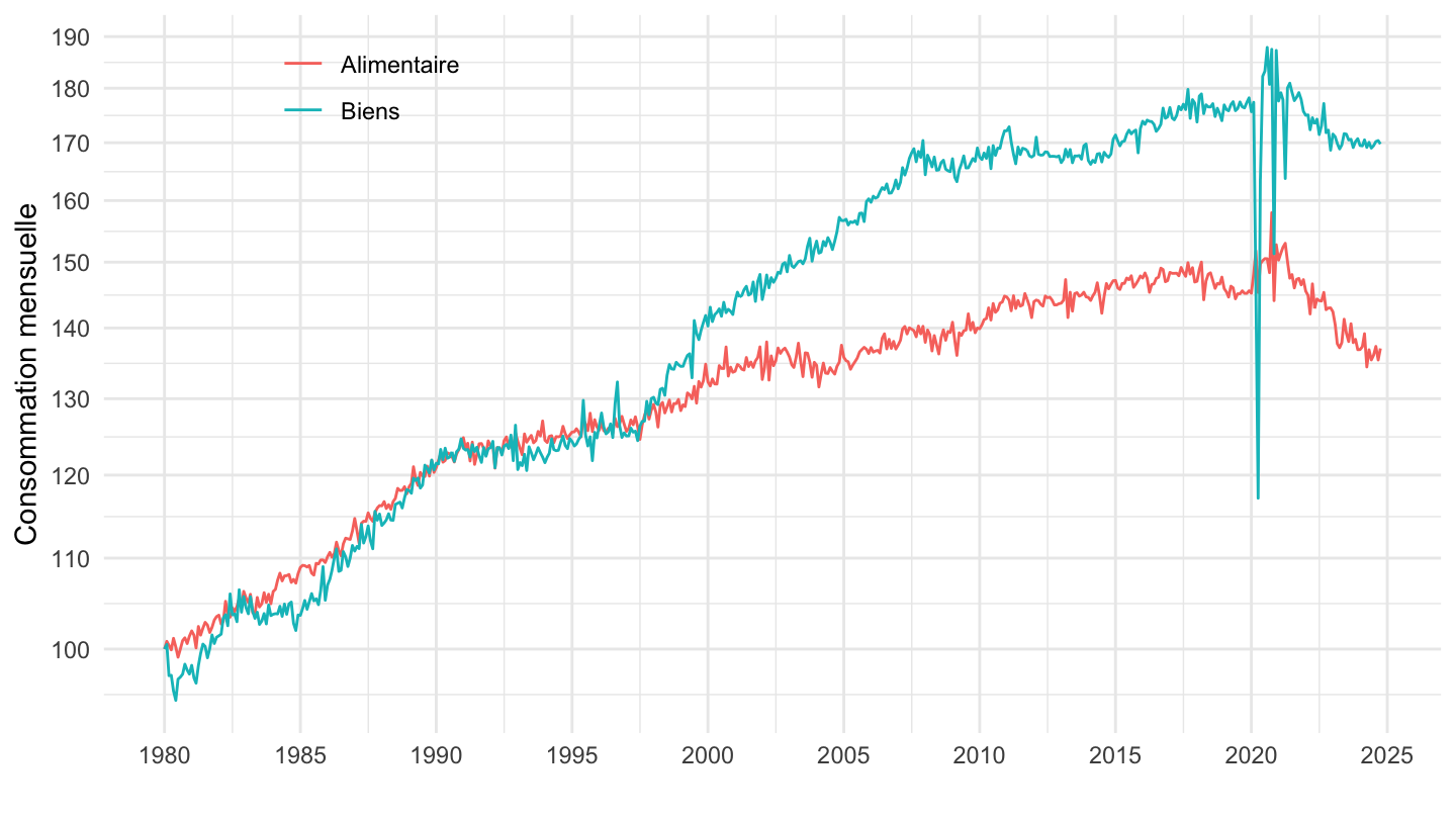
1996-
Code
`CONSO-MENAGES-2020` %>%
  filter(PRODUIT_CONSO_MENAGES %in% c("BIENS", "ALIMENTAIRE")) %>%

  month_to_date %>%
  filter(date >= as.Date("1996-01-01")) %>%
  group_by(Produit_conso_menages) %>%
  arrange(date) %>%
  mutate(OBS_VALUE = 100*OBS_VALUE/OBS_VALUE[1]) %>%
  ggplot + geom_line(aes(x = date, y = OBS_VALUE, color = Produit_conso_menages)) +
  theme_minimal() + ylab("Consommation mensuelle") + xlab("") +
  theme(legend.title = element_blank(),
        legend.position = c(0.2, 0.9)) +
  scale_x_date(breaks = seq(1950, 2030, 2) %>% paste0("-01-01") %>% as.Date,
               labels = date_format("%Y")) +
  scale_y_log10(breaks = seq(10, 300, 10))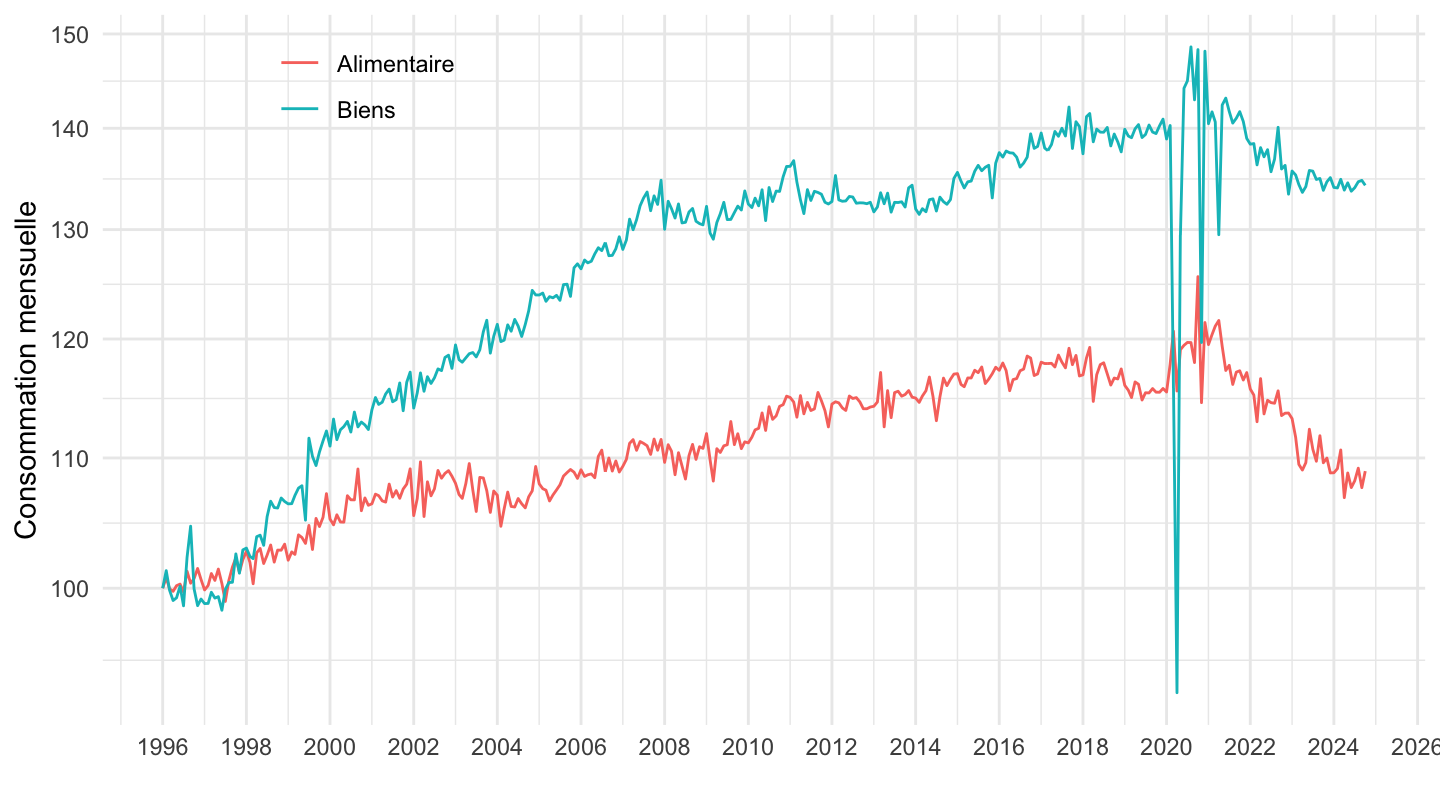
2005-
Code
`CONSO-MENAGES-2020` %>%
  filter(PRODUIT_CONSO_MENAGES %in% c("BIENS", "ALIMENTAIRE")) %>%

  month_to_date %>%
  filter(date >= as.Date("2005-01-01")) %>%
  group_by(Produit_conso_menages) %>%
  arrange(date) %>%
  mutate(OBS_VALUE = 100*OBS_VALUE/OBS_VALUE[1]) %>%
  ggplot + geom_line(aes(x = date, y = OBS_VALUE, color = Produit_conso_menages)) +
  theme_minimal() + ylab("Consommation mensuelle") + xlab("") +
  theme(legend.title = element_blank(),
        legend.position = c(0.2, 0.9)) +
  scale_x_date(breaks = seq(1950, 2030, 2) %>% paste0("-01-01") %>% as.Date,
               labels = date_format("%Y")) +
  scale_y_log10(breaks = seq(10, 300, 10))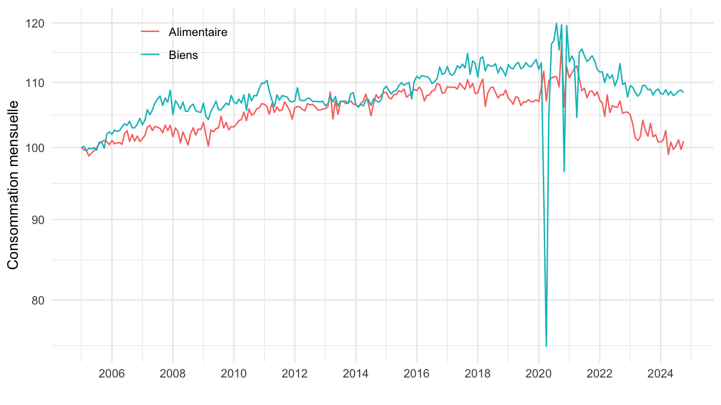
2017-
Code
`CONSO-MENAGES-2020` %>%
  filter(PRODUIT_CONSO_MENAGES %in% c("BIENS", "ALIMENTAIRE")) %>%

  month_to_date %>%
  filter(date >= as.Date("2017-01-01")) %>%
  group_by(Produit_conso_menages) %>%
  arrange(date) %>%
  mutate(OBS_VALUE = 100*OBS_VALUE/OBS_VALUE[1]) %>%
  ggplot + geom_line(aes(x = date, y = OBS_VALUE, color = Produit_conso_menages)) +
  theme_minimal() + ylab("Consommation mensuelle") + xlab("") +
  theme(legend.title = element_blank(),
        legend.position = c(0.2, 0.3)) +
  scale_x_date(breaks = seq(1950, 2030, 1) %>% paste0("-01-01") %>% as.Date,
               labels = date_format("%Y")) +
  scale_y_log10(breaks = seq(10, 300, 5))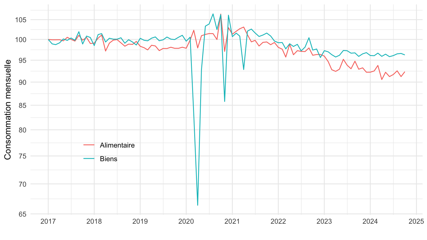
Mai 2020-
Code
Sys.setlocale("LC_TIME", "fr_CA.UTF-8")# [1] "fr_CA.UTF-8"Code
`CONSO-MENAGES-2020` %>%
  filter(PRODUIT_CONSO_MENAGES %in% c("BIENS", "ALIMENTAIRE")) %>%

  month_to_date %>%
  filter(date >= as.Date("2020-05-01")) %>%
  group_by(Produit_conso_menages) %>%
  arrange(date) %>%
  mutate(OBS_VALUE = 100*OBS_VALUE/OBS_VALUE[1]) %>%
  ggplot + geom_line(aes(x = date, y = OBS_VALUE, color = Produit_conso_menages)) +
  theme_minimal() + ylab("Consommation mensuelle") + xlab("") +
  theme(legend.title = element_blank(),
               axis.text.x = element_text(angle = 45, vjust = 1, hjust = 1),
        legend.position = c(0.2, 0.1)) +
  scale_x_date(breaks = "3 months",
               labels = date_format("%b %Y")) +
  scale_y_log10(breaks = seq(10, 300, 5))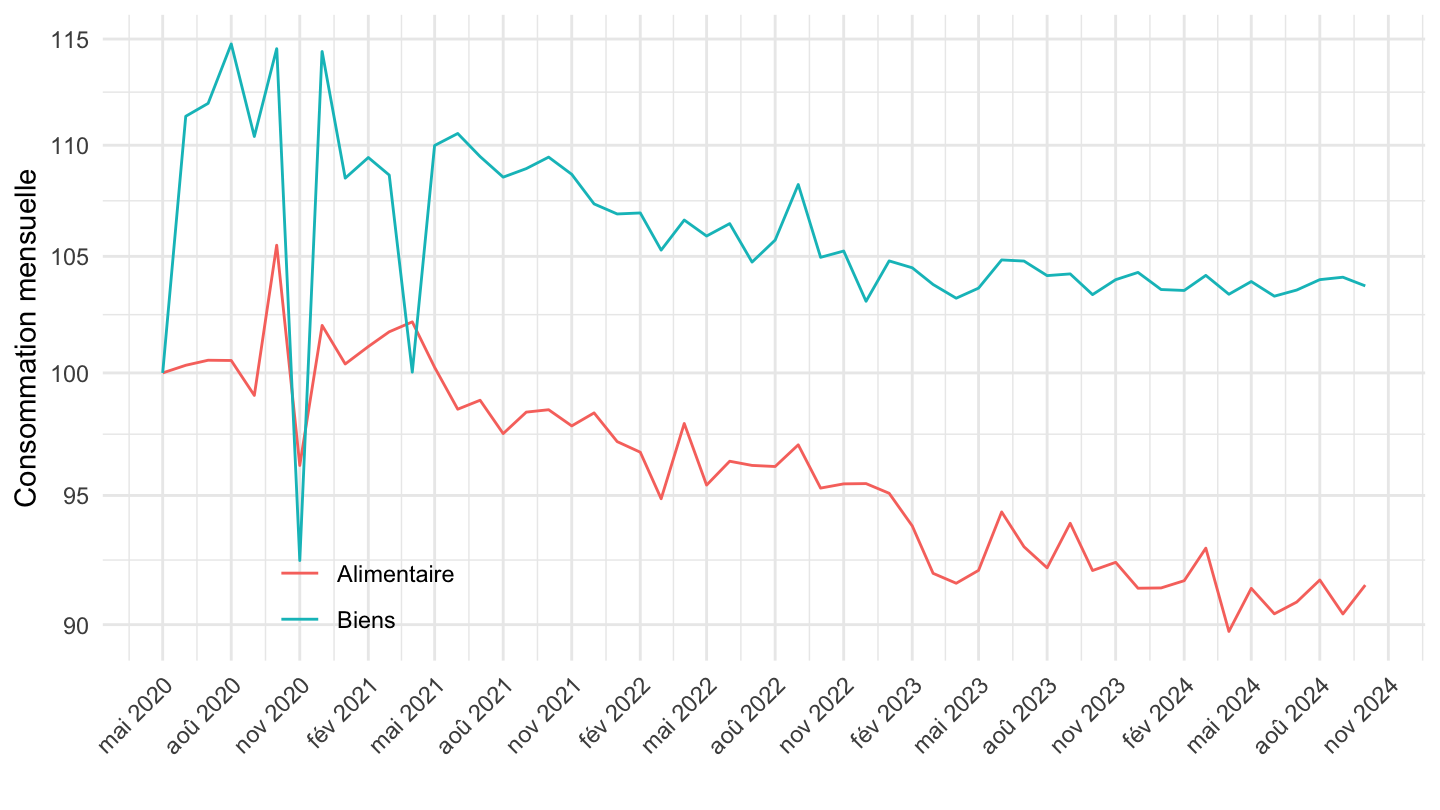
Dec 2021-
Code
Sys.setlocale("LC_TIME", "fr_CA.UTF-8")# [1] "fr_CA.UTF-8"Code
`CONSO-MENAGES-2020` %>%
  filter(PRODUIT_CONSO_MENAGES %in% c("BIENS", "ALIMENTAIRE", "ALIMENTAIRE-HORS-TABAC")) %>%

  month_to_date %>%
  filter(date >= as.Date("2022-01-01")) %>%
  group_by(Produit_conso_menages) %>%
  arrange(date) %>%
  mutate(OBS_VALUE = OBS_VALUE/OBS_VALUE[1]-1) %>%
  ggplot + geom_line(aes(x = date, y = OBS_VALUE, color = Produit_conso_menages)) +
  theme_minimal() + ylab("Consommation mensuelle (par rapport à Janvier 2022)") + xlab("") +
  theme(legend.title = element_blank(),
               axis.text.x = element_text(angle = 45, vjust = 1, hjust = 1),
        legend.position = c(0.2, 0.2)) +
  scale_x_date(breaks = "1 month",
               labels = date_format("%B %Y")) +
  scale_y_continuous(breaks = 0.01*seq(-100, 300, 1),
                labels = percent_format(acc = 1))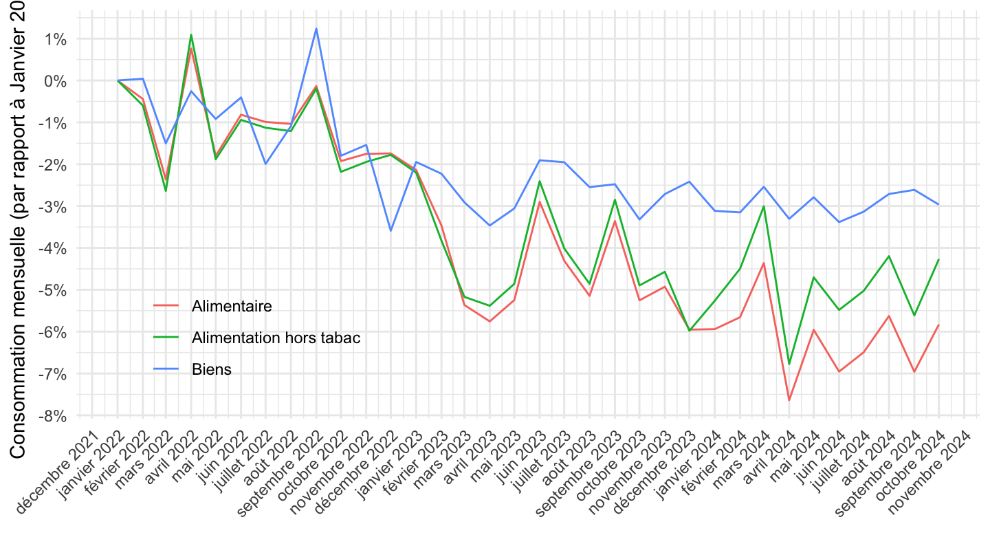
Feb 2022
Code
Sys.setlocale("LC_TIME", "fr_CA.UTF-8")# [1] "fr_CA.UTF-8"Code
`CONSO-MENAGES-2020` %>%
  filter(PRODUIT_CONSO_MENAGES %in% c("BIENS", "ALIMENTAIRE", "ALIMENTAIRE-HORS-TABAC")) %>%

  month_to_date %>%
  filter(date >= as.Date("2022-02-01")) %>%
  group_by(Produit_conso_menages) %>%
  arrange(date) %>%
  mutate(OBS_VALUE = OBS_VALUE/OBS_VALUE[1]-1) %>%
  ggplot + geom_line(aes(x = date, y = OBS_VALUE, color = Produit_conso_menages)) +
  theme_minimal() + ylab("Consommation mensuelle (vs. Fév. 2022)") + xlab("") +
  theme(legend.title = element_blank(),
               axis.text.x = element_text(angle = 45, vjust = 1, hjust = 1),
        legend.position = c(0.2, 0.2)) +
  scale_x_date(breaks = "1 month",
               labels = date_format("%B %Y")) +
  scale_y_continuous(breaks = 0.01*seq(-100, 300, 1),
                labels = percent_format(acc = 1))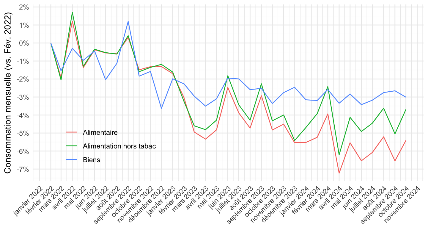
24 months
Code
Sys.setlocale("LC_TIME", "fr_CA.UTF-8")# [1] "fr_CA.UTF-8"Code
`CONSO-MENAGES-2020` %>%
  filter(PRODUIT_CONSO_MENAGES %in% c("BIENS", "ALIMENTAIRE", "ALIMENTAIRE-HORS-TABAC")) %>%

  month_to_date %>%
  filter(date >= Sys.Date() - months(24)) %>%
  group_by(Produit_conso_menages) %>%
  arrange(date) %>%
  mutate(OBS_VALUE = OBS_VALUE/OBS_VALUE[1]-1) %>%
  ggplot + geom_line(aes(x = date, y = OBS_VALUE, color = Produit_conso_menages)) +
  theme_minimal() + ylab("Consommation mensuelle (par rapport à Janvier 2022)") + xlab("") +
  theme(legend.title = element_blank(),
               axis.text.x = element_text(angle = 45, vjust = 1, hjust = 1),
        legend.position = c(0.2, 0.2)) +
  scale_x_date(breaks = "1 month",
               labels = date_format("%B %Y")) +
  scale_y_continuous(breaks = 0.01*seq(-100, 300, 1),
                labels = percent_format(acc = 1))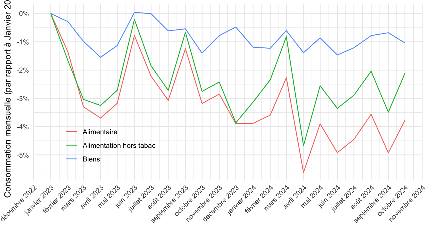
18 months
Code
Sys.setlocale("LC_TIME", "fr_CA.UTF-8")# [1] "fr_CA.UTF-8"Code
`CONSO-MENAGES-2020` %>%
  filter(PRODUIT_CONSO_MENAGES %in% c("BIENS", "ALIMENTAIRE", "ALIMENTAIRE-HORS-TABAC")) %>%

  month_to_date %>%
  filter(date >= Sys.Date() - months(18)) %>%
  group_by(Produit_conso_menages) %>%
  arrange(date) %>%
  mutate(OBS_VALUE = OBS_VALUE/OBS_VALUE[1]-1) %>%
  ggplot + geom_line(aes(x = date, y = OBS_VALUE, color = Produit_conso_menages)) +
  theme_minimal() + ylab("Consommation mensuelle (par rapport à Janvier 2022)") + xlab("") +
  theme(legend.title = element_blank(),
               axis.text.x = element_text(angle = 45, vjust = 1, hjust = 1),
        legend.position = c(0.2, 0.2)) +
  scale_x_date(breaks = "1 month",
               labels = date_format("%B %Y")) +
  scale_y_continuous(breaks = 0.01*seq(-100, 300, 1),
                labels = percent_format(acc = 1))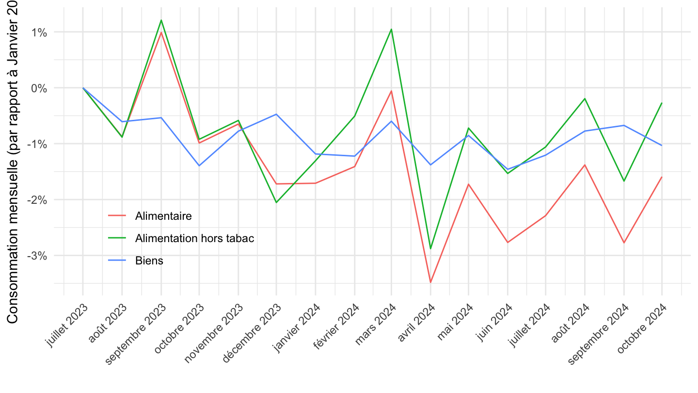
Biens, Biens Manufacturés, Biens Fabriqués
All
Code
`CONSO-MENAGES-2020` %>%
  filter(PRODUIT_CONSO_MENAGES %in% c("BIENS", "BIENS-MANUFACTURES", "BIENS-FABRIQUES")) %>%

  month_to_date %>%
  ggplot + geom_line(aes(x = date, y = OBS_VALUE, color = Produit_conso_menages)) +
  xlab("") + ylab("") +  theme_minimal() +
  scale_x_date(breaks = "5 years",
               labels = date_format("%Y")) +
  scale_y_log10(breaks = seq(0, 120, 5)) +
  theme(legend.position = c(0.8, 0.2),
        legend.title = element_blank())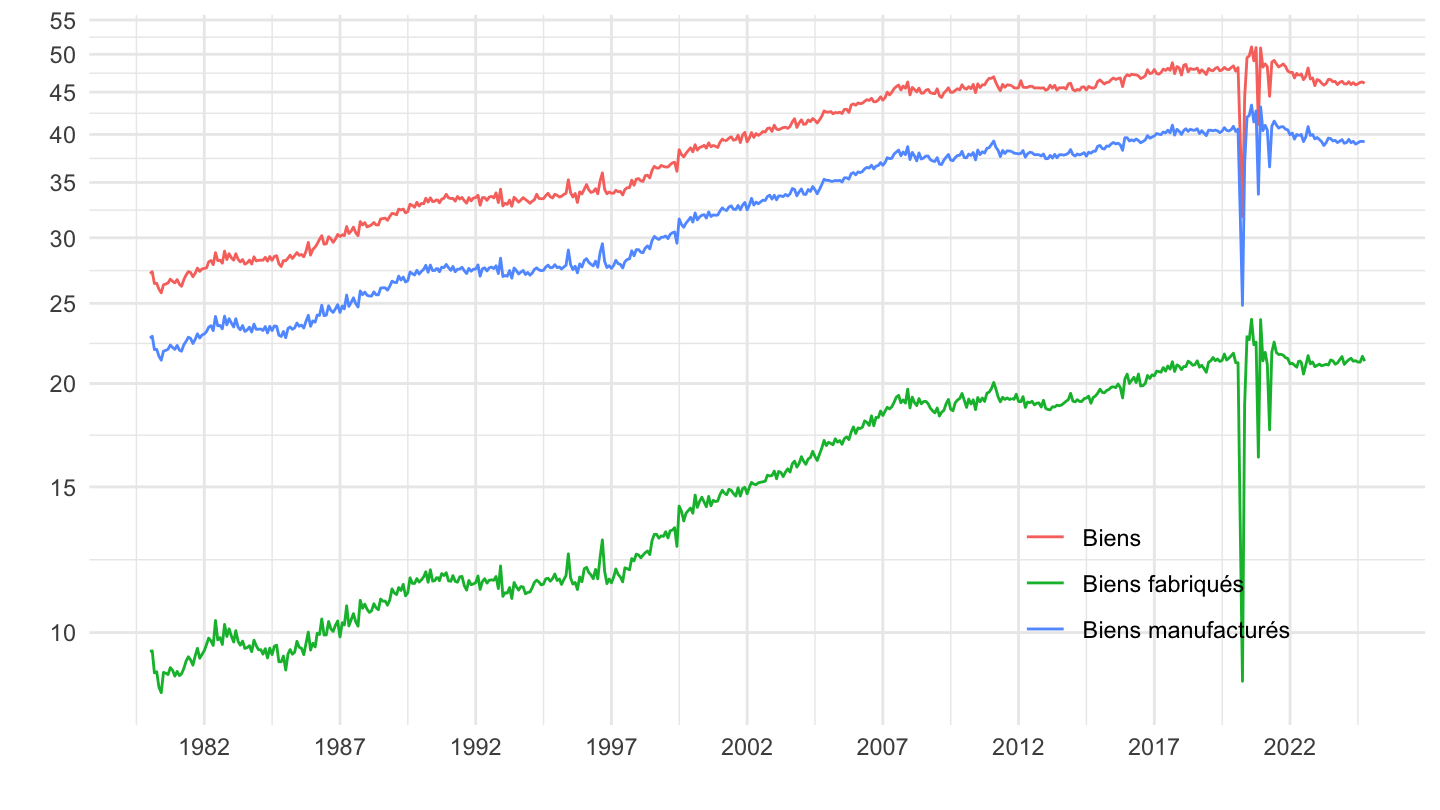
1996-
Code
`CONSO-MENAGES-2020` %>%
  filter(PRODUIT_CONSO_MENAGES %in% c("BIENS", "BIENS-MANUFACTURES", "BIENS-FABRIQUES")) %>%

  month_to_date %>%
  filter(date >= as.Date("1996-01-01")) %>%
  ggplot + geom_line(aes(x = date, y = OBS_VALUE, color = Produit_conso_menages)) +
  xlab("") + ylab("") +  theme_minimal() +
  scale_x_date(breaks = seq(1920, 2025, 2) %>% paste0("-01-01") %>% as.Date,
               labels = date_format("%Y")) +
  scale_y_log10(breaks = seq(0, 120, 5)) +

  theme(legend.position = c(0.8, 0.2),
        legend.title = element_blank())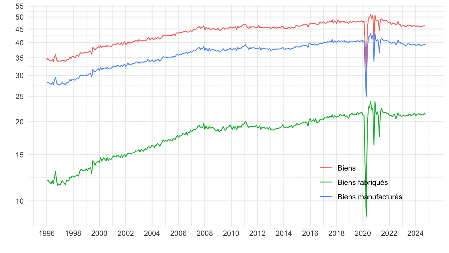
Alimentaire, Alimentaire hors Tabac, Biens durables
All
Code
`CONSO-MENAGES-2020` %>%
  filter(PRODUIT_CONSO_MENAGES %in% c("ALIMENTAIRE", "ALIMENTAIRE-HORS-TABAC", "BIENS-DURABLES")) %>%

  month_to_date %>%
  ggplot + geom_line(aes(x = date, y = OBS_VALUE, color = Produit_conso_menages)) +
  xlab("") + ylab("") +  theme_minimal() +
  scale_x_date(breaks = seq(1920, 2025, 5) %>% paste0("-01-01") %>% as.Date,
               labels = date_format("%Y")) +
  scale_y_log10(breaks = seq(0, 120, 1)) +

  theme(legend.position = c(0.8, 0.2),
        legend.title = element_blank())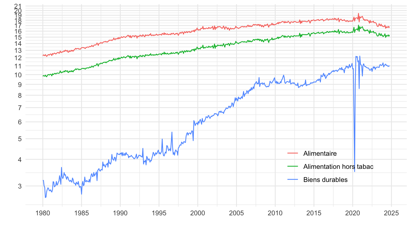
Equipement du logement, Matériels de Transport
Code
`CONSO-MENAGES-2020` %>%
  filter(PRODUIT_CONSO_MENAGES %in% c("MATERIELS-TRANSPORT", "EQUIPEMENT-LOGEMENT")) %>%

  month_to_date %>%
  ggplot + geom_line(aes(x = date, y = OBS_VALUE, color = Produit_conso_menages)) +
  xlab("") + ylab("") +  theme_minimal() +
  scale_x_date(breaks = seq(1920, 2025, 5) %>% paste0("-01-01") %>% as.Date,
               labels = date_format("%Y")) +
  scale_y_log10(breaks = seq(0, 120, 1)) +
  scale_color_manual(values = viridis(3)[1:2]) +
  theme(legend.position = c(0.8, 0.2),
legend.title = element_blank())![]()
Dec 2021
Table
Code
`CONSO-MENAGES-2020` %>%

  filter(TIME_PERIOD %in% c("2021-12", "2023-05")) %>%
  select(TIME_PERIOD, PRODUIT_CONSO_MENAGES, Produit_conso_menages, OBS_VALUE) %>%
  spread(TIME_PERIOD, OBS_VALUE) %>%
  mutate(croissance = round(100*(`2023-05`/`2021-12`-1), 1)) %>%
  arrange(croissance) %>%
print_table_conditional()| PRODUIT_CONSO_MENAGES | Produit_conso_menages | 2021-12 | 2023-05 | croissance |
|---|---|---|---|---|
| ALIMENTAIRE | Alimentaire | 18.146 | 16.833 | -7.2 |
| ALIMENTAIRE-HORS-TABAC | Alimentation hors tabac | 16.314 | 15.181 | -6.9 |
| ENERGIE_C2 | Cokéfaction et raffinage (C2) | 3.737 | 3.588 | -4.0 |
| PRODUITS-PETROLIERS | Produits pétroliers | 4.587 | 4.415 | -3.7 |
| EQUIPEMENT-LOGEMENT | Équipement du logement | 3.747 | 3.641 | -2.8 |
| BIENS | Biens | 47.639 | 46.386 | -2.6 |
| BIENS-MANUFACTURES | Biens manufacturés | 40.443 | 39.464 | -2.4 |
| BIENS-FABRIQUES-AUTRES | Autres biens fabriqués | 6.394 | 6.246 | -2.3 |
| ENERGIE_DEC2 | Énergie, eau, déchets, cokéfaction et raffinage (DE, C2) | 8.231 | 8.059 | -2.1 |
| BIENS-DURABLES-EQUIPEMENT | Biens durables d'équipement personnel | 1.756 | 1.733 | -1.3 |
| ENERGIE_DE | Énergie, eau et déchets (DE) | 4.494 | 4.457 | -0.8 |
| ENERGIE_PETROLE | Énergie hors produits pétroliers | 3.643 | 3.653 | 0.3 |
| BIENS-FABRIQUES | Biens fabriqués | 21.263 | 21.542 | 1.3 |
| TEXTILE | Textile-cuir | 4.203 | 4.312 | 2.6 |
| BIENS-DURABLES | Biens durables | 10.666 | 10.988 | 3.0 |
| MATERIELS-TRANSPORT | Matériels de transport | 5.163 | 5.612 | 8.7 |
Graph
Code
Sys.setlocale("LC_TIME", "fr_CA.UTF-8")# [1] "fr_CA.UTF-8"Code
`CONSO-MENAGES-2020` %>%

  month_to_date %>%
  filter(date >= as.Date("2022-01-01")) %>%
  group_by(Produit_conso_menages) %>%
  arrange(date) %>%
  mutate(OBS_VALUE = 100*OBS_VALUE/OBS_VALUE[1]) %>%
  ggplot + geom_line(aes(x = date, y = OBS_VALUE, color = Produit_conso_menages)) +
  theme_minimal() + ylab("Consommation mensuelle (Base 100 = Déc. 2021)") + xlab("") +
  theme(legend.title = element_blank(),
               axis.text.x = element_text(angle = 45, vjust = 1, hjust = 1),
        legend.position = c(0.5, 0.3)) +
  scale_x_date(breaks = "1 month",
               labels = date_format("%B %Y")) +
  scale_y_log10(breaks = seq(10, 300, 1)) +
  guides(color=guide_legend(ncol=2))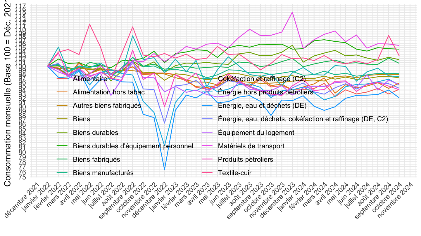
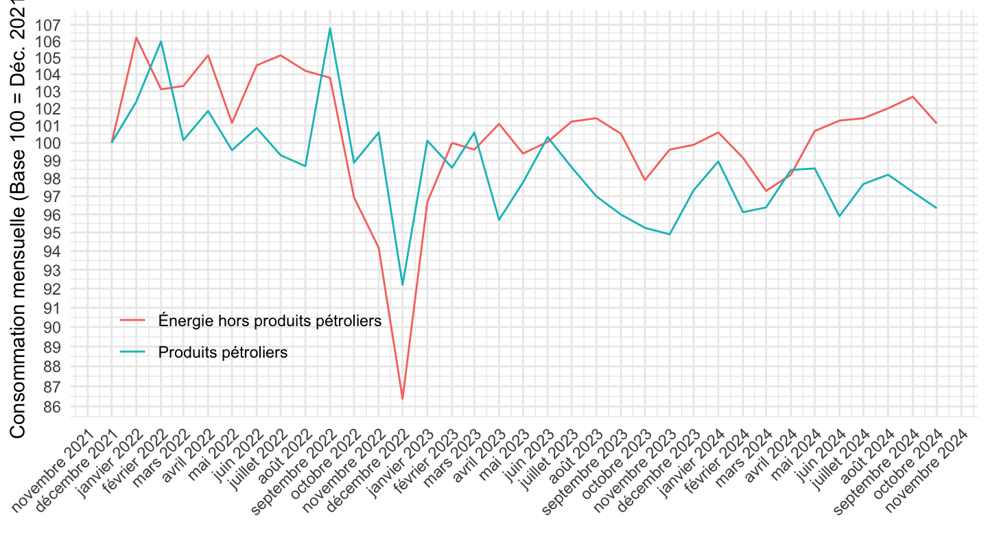
Produits pétroliers
Code
Sys.setlocale("LC_TIME", "fr_CA.UTF-8")# [1] "fr_CA.UTF-8"Code
`CONSO-MENAGES-2020` %>%
  filter(PRODUIT_CONSO_MENAGES %in% c("PRODUITS-PETROLIERS", "ENERGIE_PETROLE")) %>%

  month_to_date %>%
  filter(date >= as.Date("2021-12-01")) %>%
  group_by(Produit_conso_menages) %>%
  arrange(date) %>%
  mutate(OBS_VALUE = 100*OBS_VALUE/OBS_VALUE[1]) %>%
  ggplot + geom_line(aes(x = date, y = OBS_VALUE, color = Produit_conso_menages)) +
  theme_minimal() + ylab("Consommation mensuelle (Base 100 = Déc. 2021)") + xlab("") +
  theme(legend.title = element_blank(),
               axis.text.x = element_text(angle = 45, vjust = 1, hjust = 1),
        legend.position = c(0.2, 0.2)) +
  scale_x_date(breaks = "1 month",
               labels = date_format("%B %Y")) +
  scale_y_log10(breaks = seq(10, 300, 1))