
Last observation: 2025 (N = 21)
First observation: 1949 (N = 5)
Last data update: 15 oct. 2026, 23:08
Last compile: 16 oct. 2026, 01:28
Base = un ensemble fixé de concepts, nomenclatures, et méthodes. (dans le vocabulaire de la Comptabilité Nationale Française (CNF))
Création de la CNF dans les années 1950.
Changements de base: 1956, 1959, 1962, 1971, 1980, 1995, 2000, 2005, 2010, 2014
Les comptes de la nation en 2022. html
`CNA-2020-PIB` |>
  filter(TIME_PERIOD == max(TIME_PERIOD)) |>
  select(TIME_PERIOD, TITLE_FR, OBS_VALUE) |>
print_table_conditional()| TIME_PERIOD | TITLE_FR | OBS_VALUE |
|---|---|---|
| 2025 | Comptes nationaux annuels base 2020 - Dépense de consommation finale - APU Administrations publiques - Total des produits (nouvelle nomenclature) - Contribution à l'évolution du produit intérieur brut en volume | 0.146 |
| 2025 | Comptes nationaux annuels base 2020 - Importations de biens et de services - Total des secteurs institutionnels - Total des produits (nouvelle nomenclature) - Contribution à l'évolution du produit intérieur brut en volume | -0.958 |
| 2025 | Comptes nationaux annuels base 2020 - Formation brute de capital fixe - APU Administrations publiques - Total des produits (nouvelle nomenclature) - Contribution à l'évolution du produit intérieur brut en volume | 0.115 |
| 2025 | Comptes nationaux annuels base 2020 - Formation brute de capital fixe - Ménages hors entrepreneurs individuels - Total des produits (nouvelle nomenclature) - Contribution à l'évolution du produit intérieur brut en volume | -0.009 |
| 2025 | Comptes nationaux annuels base 2020 - Produit intérieur brut approche produit - Total des secteurs institutionnels - Total des produits - Prix chaîné année de base (non équilibré) | 2646746.000 |
| 2025 | Comptes nationaux annuels base 2020 - Produit intérieur brut approche produit - Total des secteurs institutionnels - Total des produits - Prix courant | 2991056.000 |
| 2025 | Comptes nationaux annuels base 2020 - Produit intérieur brut approche produit - Total des secteurs institutionnels - Total des produits - Indice de prix chaîné année de base (non équilibré) | 113.000 |
| 2025 | Comptes nationaux annuels base 2020 - Formation brute de capital fixe - Sociétés et E.I. financières - Total des produits (nouvelle nomenclature) - Contribution à l'évolution du produit intérieur brut en volume | -0.053 |
| 2025 | Comptes nationaux annuels base 2020 - Formation brute de capital fixe - Total des secteurs institutionnels - Total des produits (nouvelle nomenclature) - Contribution à l'évolution du produit intérieur brut en volume | 0.107 |
| 2025 | Comptes nationaux annuels base 2020 - Acquisitions moins cessions d'objets de valeur - Total des secteurs institutionnels - Total des produits (nouvelle nomencl.) - Contribution à l'évolution du produit intérieur brut en volume | -0.002 |
| 2025 | Comptes nationaux annuels base 2020 - Dépense de consommation finale - Total des secteurs institutionnels - Total des produits (nouvelle nomenclature) - Contribution à l'évolution du produit intérieur brut en volume | 0.343 |
| 2025 | Comptes nationaux annuels base 2020 - Dépense de consommation finale - Instituts sans but lucratif au service des ménages - Total des produits (nouvelle nomenclature) - Contribution à l'évolution du produit intérieur brut en volume | -0.005 |
| 2025 | Comptes nationaux annuels base 2020 - Produit intérieur brut par habitant - Total des secteurs institutionnels - Total des produits (nouvelle nomenclature) - Prix courant | 43350.238 |
| 2025 | Comptes nationaux annuels base 2020 - Formation brute de capital fixe - Sociétés et E.I. non financières - Total des produits (nouvelle nomenclature) - Contribution à l'évolution du produit intérieur brut en volume | 0.054 |
| 2025 | Comptes nationaux annuels base 2020 - Formation brute de capital fixe - Instituts sans but lucratif au service des ménages - Total des produits (nouvelle nomenclature) - Contribution à l'évolution du produit intérieur brut en volume | 0.001 |
| 2025 | Comptes nationaux annuels base 2020 - Solde des échanges extérieurs de biens et services - Total des sect. institutionnels - Total des produits (nouvelle nomencl.) - Contribution à l'évolution du produit intérieur brut en volume | -0.172 |
| 2025 | Comptes nationaux annuels base 2020 - Variation des stocks - Total des secteurs institutionnels - Total des produits (nouvelle nomenclature) - Contribution à l'évolution du produit intérieur brut en volume | 0.528 |
| 2025 | Comptes nationaux annuels base 2020 - Produit intérieur brut - Evolution en volume - Prix chaîné année de base (non équilibré) | 0.805 |
| 2025 | Comptes nationaux annuels base 2020 - Produit intérieur brut par habitant - Total des secteurs institutionnels - Total des produits (nouvelle nomenclature) - Prix chaîné année de base (non équilibré) | 38360.050 |
| 2025 | Comptes nationaux annuels base 2020 - Dépense de consommation finale - Ménages hors entrepreneurs individuels - Total des produits (nouvelle nomenclature) - Contribution à l'évolution du produit intérieur brut en volume | 0.202 |
| 2025 | Comptes nationaux annuels base 2020 - Exportations de biens et de services - Total des secteurs institutionnels - Total des produits (nouvelle nomenclature) - Contribution à l'évolution du produit intérieur brut en volume | 0.786 |
SECT-INST, UNIT_MEASURE`CNA-2020-PIB` |>
group_by(OPERATION, NATURE, `SECT-INST`, UNIT_MEASURE) |>
summarise(Nobs = n()) %>%
mutate_at(vars(-Nobs, -OPERATION), funs(as.factor(.))) |>
arrange(-Nobs) |>
print_table_conditional()| OPERATION | NATURE | SECT-INST | UNIT_MEASURE | Nobs |
|---|---|---|---|---|
| PIB_H | VALEUR_ABSOLUE | S0 | EUROS_HABITANTS | 154 |
| PIB | INDICE | S0 | SO | 77 |
| PIB | VALEUR_ABSOLUE | S0 | EUR2020 | 77 |
| PIB | VALEUR_ABSOLUE | S0 | EUROS_COURANTS | 77 |
| B11 | PROPORTION_POURCENTAGE | S0 | SO | 76 |
| P3 | PROPORTION_POURCENTAGE | S0 | SO | 76 |
| P3 | PROPORTION_POURCENTAGE | S13 | SO | 76 |
| P3 | PROPORTION_POURCENTAGE | S14B | SO | 76 |
| P3 | PROPORTION_POURCENTAGE | S15 | SO | 76 |
| P51G | PROPORTION_POURCENTAGE | S0 | SO | 76 |
| P51G | PROPORTION_POURCENTAGE | S11ES14AA | SO | 76 |
| P51G | PROPORTION_POURCENTAGE | S12ES14AF | SO | 76 |
| P51G | PROPORTION_POURCENTAGE | S13 | SO | 76 |
| P51G | PROPORTION_POURCENTAGE | S14B | SO | 76 |
| P51G | PROPORTION_POURCENTAGE | S15 | SO | 76 |
| P52 | PROPORTION_POURCENTAGE | S0 | SO | 76 |
| P53 | PROPORTION_POURCENTAGE | S0 | SO | 76 |
| P6 | PROPORTION_POURCENTAGE | S0 | SO | 76 |
| P7 | PROPORTION_POURCENTAGE | S0 | SO | 76 |
| PIB | PROPORTION_POURCENTAGE | S0 | POURCENT | 76 |
`CNA-2020-PIB` |>
  year_to_date() |>
  filter(OPERATION == "PIB",
         UNIT_MEASURE %in% c("EUR2020", "EUROS_COURANTS")) |>
  select(date, UNIT_MEASURE, OBS_VALUE) |>
  mutate(OBS_VALUE = OBS_VALUE |> as.numeric(),
         UNIT_MEASURE = paste0("PIB_", UNIT_MEASURE)) |>
  spread(UNIT_MEASURE, OBS_VALUE) |>
print_table_conditional()`CNA-2020-PIB` |>
filter(as.numeric(TIME_PERIOD) >= 2017) |>
filter(OPERATION == "PIB",
UNIT_MEASURE %in% c("EUR2020", "EUROS_COURANTS")) |>
select(TIME_PERIOD, UNIT_MEASURE, OBS_VALUE) |>
mutate(OBS_VALUE = OBS_VALUE |> as.numeric(),
UNIT_MEASURE = paste0("PIB_", UNIT_MEASURE)) |>
spread(UNIT_MEASURE, OBS_VALUE) |>
print_table_conditional()| TIME_PERIOD | PIB_EUR2020 | PIB_EUROS_COURANTS |
|---|---|---|
| 2017 | 2415116 | 2291681 |
| 2018 | 2454866 | 2355363 |
| 2019 | 2504637 | 2432207 |
| 2020 | 2318276 | 2318276 |
| 2021 | 2477828 | 2508102 |
| 2022 | 2545145 | 2653997 |
| 2023 | 2586706 | 2833826 |
| 2024 | 2625622 | 2935236 |
| 2025 | 2646746 | 2991056 |
`CNA-2020-PIB` |>
  filter(OPERATION == "PIB",
         UNIT_MEASURE == "EUROS_COURANTS") |>
  select(TIME_PERIOD, `PIB Nominal` = OBS_VALUE) |>
  year_to_date() |>
  mutate(year = year(date)) |>
  filter(is.finite(`PIB Nominal`)) |>
  group_by(date) |>
  select(-year) |>
  gather(variable, value, -date) |>
  ggplot() + theme_minimal() + xlab("") + ylab("PIB nominal de la France (en € courants)") +
  geom_line(aes(x = date, y = value/10^3, color = variable, linetype = variable)) +
  scale_linetype_manual(values = c("solid", "solid", "dashed", "solid")) +
  theme(legend.title = element_blank(),
        legend.position = c(0.8, 0.2)) +
  scale_x_date(breaks = seq(1920, 2100, 5) |> paste0("-01-01") |> as.Date(),
               labels = date_format("%Y")) +
  scale_y_continuous(breaks = seq(200, 3000, 200),
                labels = scales::dollar_format(a = 1, prefix = "", suffix = "Md€"))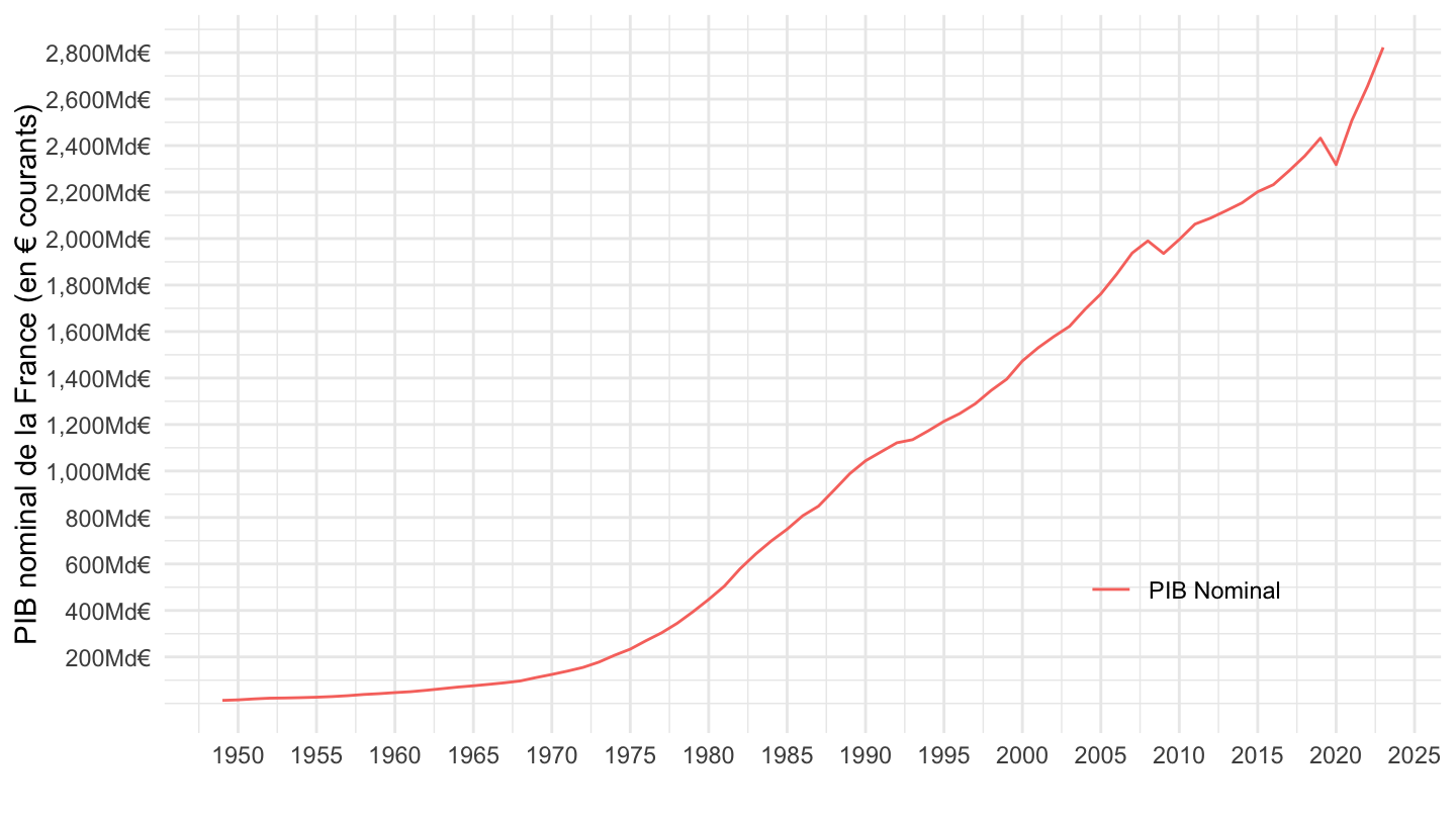
fit <- `CNA-2020-PIB` |>
  filter(OPERATION == "PIB",
         UNIT_MEASURE == "EUR2020") |>
  select(TIME_PERIOD, `Real GDP` = OBS_VALUE) |>
  year_to_date() |>
  mutate(year = year(date)) |>
  filter(is.finite(`Real GDP`))  |>
  filter(year <= 1971) %>%
  lm(log(`Real GDP`) ~ year, data = .) |>
  pluck("coefficients")


fit_2019 <- `CNA-2020-PIB` |>
  filter(OPERATION == "PIB",
         UNIT_MEASURE == "EUR2020") |>
  select(TIME_PERIOD, `Real GDP` = OBS_VALUE) |>
  year_to_date() |>
  mutate(year = year(date)) |>
  filter(is.finite(`Real GDP`)) %>%
  lm(log(`Real GDP`) ~ year, data = .) |>
  pluck("coefficients")

fit
# (Intercept) year
# -87.4994240 0.0513393fit_2019# (Intercept) year
# -42.17299922 0.02827044`CNA-2020-PIB` |>
filter(OPERATION == "PIB",
UNIT_MEASURE == "EUR2020") |>
select(TIME_PERIOD, `Real GDP` = OBS_VALUE) |>
year_to_date() |>
mutate(year = year(date)) |>
filter(is.finite(`Real GDP`)) |>
mutate(`Trend to 2024 (g = 2.9%)` = lm(log(`Real GDP`) ~ year) |> fitted() |> exp(),
`Trend to 1971, extrapolated` = ifelse(year>=1971,
(fit[1]+fit[2]*year) |> exp(),
NA),
`Trend to 1971 (g = 5.1%)` = ifelse(year<=1971,
(fit[1]+fit[2]*year) |> exp(),
NA)) |>
group_by(date) |>
select(-year) |>
gather(variable, value, -date) |>
ggplot() + theme_minimal() + xlab("") + ylab("France's GDP") +
geom_line(aes(x = date, y = value/10^6, color = variable, linetype = variable)) +
scale_color_manual(values = viridis(4)[c(3, 1, 1, 2)]) +
scale_linetype_manual(values = c("solid", "solid", "dashed", "solid")) +
theme(legend.title = element_blank(),
legend.position = c(0.8, 0.2)) +
scale_x_date(breaks = seq(1920, 2100, 5) |> paste0("-01-01") |> as.Date(),
labels = date_format("%Y")) +
scale_y_log10(breaks = 20*2^seq(-7, 1, 1),
labels = scales::dollar_format(a = .1, prefix = "", suffix = "Tn€"))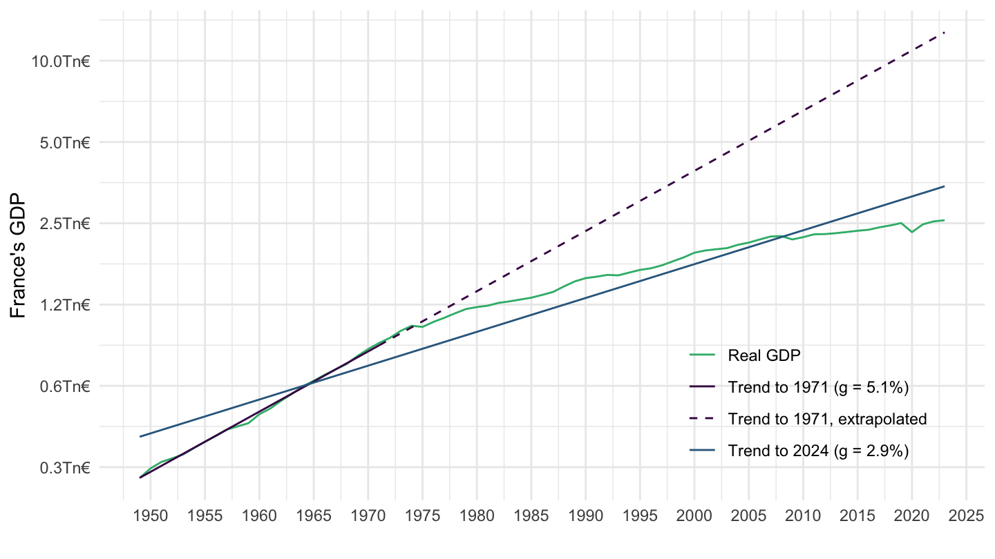
plot_lineaire <- `CNA-2020-PIB` |>
  filter(OPERATION %in% c("PIB", "P3"),
         UNIT_MEASURE == "EUR2020") |>

  year_to_date() |>
  mutate(year = year(date)) |>
  group_by(date) |>
  select(-year) |>
  ggplot() + theme_minimal() + xlab("") + ylab("PIB réel de la France (en € 2020)") +
  geom_line(aes(x = date, y = OBS_VALUE/10^3, color = Operation)) +
  scale_linetype_manual(values = c("solid", "solid", "dashed", "solid")) +
  theme(legend.title = element_blank(),
        legend.position = c(0.8, 0.2)) +
  scale_x_date(breaks = seq(1920, 2100, 10) |> paste0("-01-01") |> as.Date(),
               labels = date_format("%Y")) +
  scale_y_continuous(breaks = seq(200, 3000, 200),
                labels = scales::dollar_format(a = 1, prefix = "", suffix = "Md€"))

plot_lineaire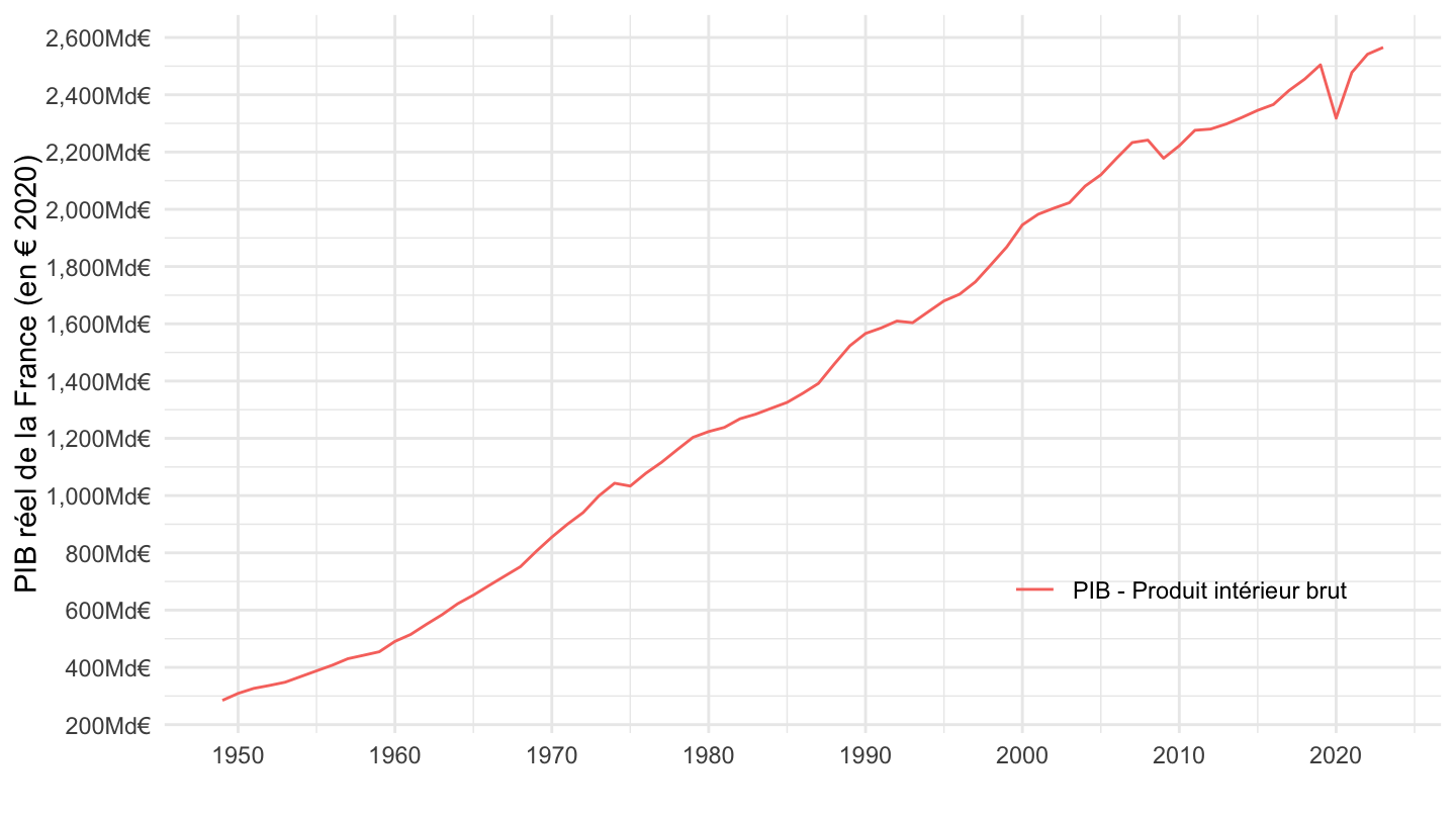
plot_log <- plot_lineaire+
  scale_y_log10(breaks = 20000*2^seq(-7, 1, 0.5),
                labels = scales::dollar_format(a = 1, prefix = "", suffix = "Md€"))

plot_log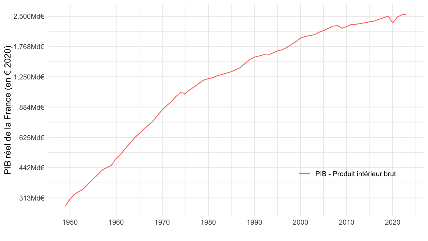
ggarrange(plot_lineaire + ggtitle("Echelle Linéaire"), plot_log + ylab("") + ggtitle("Echelle Log"), common.legend = T)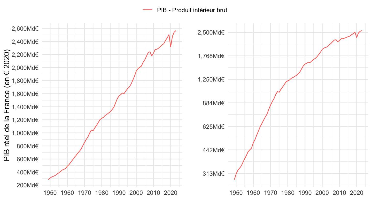
plot_lineaire <- `CNA-2020-PIB` |>
  filter(OPERATION %in% c("PIB", "P3"),
         UNIT_MEASURE == "EUR2020") |>

  year_to_date() |>
  mutate(year = year(date)) |>
  filter(year >= 1960) |>
  group_by(date) |>
  select(-year) |>
  ggplot() + theme_minimal() + xlab("") + ylab("PIB réel de la France (en € 2020)") +
  geom_line(aes(x = date, y = OBS_VALUE/10^3, color = Operation)) +
  scale_linetype_manual(values = c("solid", "solid", "dashed", "solid")) +
  theme(legend.title = element_blank(),
        legend.position = c(0.8, 0.2)) +
  scale_x_date(breaks = seq(1920, 2100, 10) |> paste0("-01-01") |> as.Date(),
               labels = date_format("%Y")) +
  scale_y_continuous(breaks = seq(200, 3000, 200),
                labels = scales::dollar_format(a = 1, prefix = "", suffix = "Md€"))

plot_lineaire
plot_log <- plot_lineaire+
  scale_y_log10(breaks = 20000*2^seq(-7, 1, 0.5),
                labels = scales::dollar_format(a = 1, prefix = "", suffix = "Md€"))

plot_log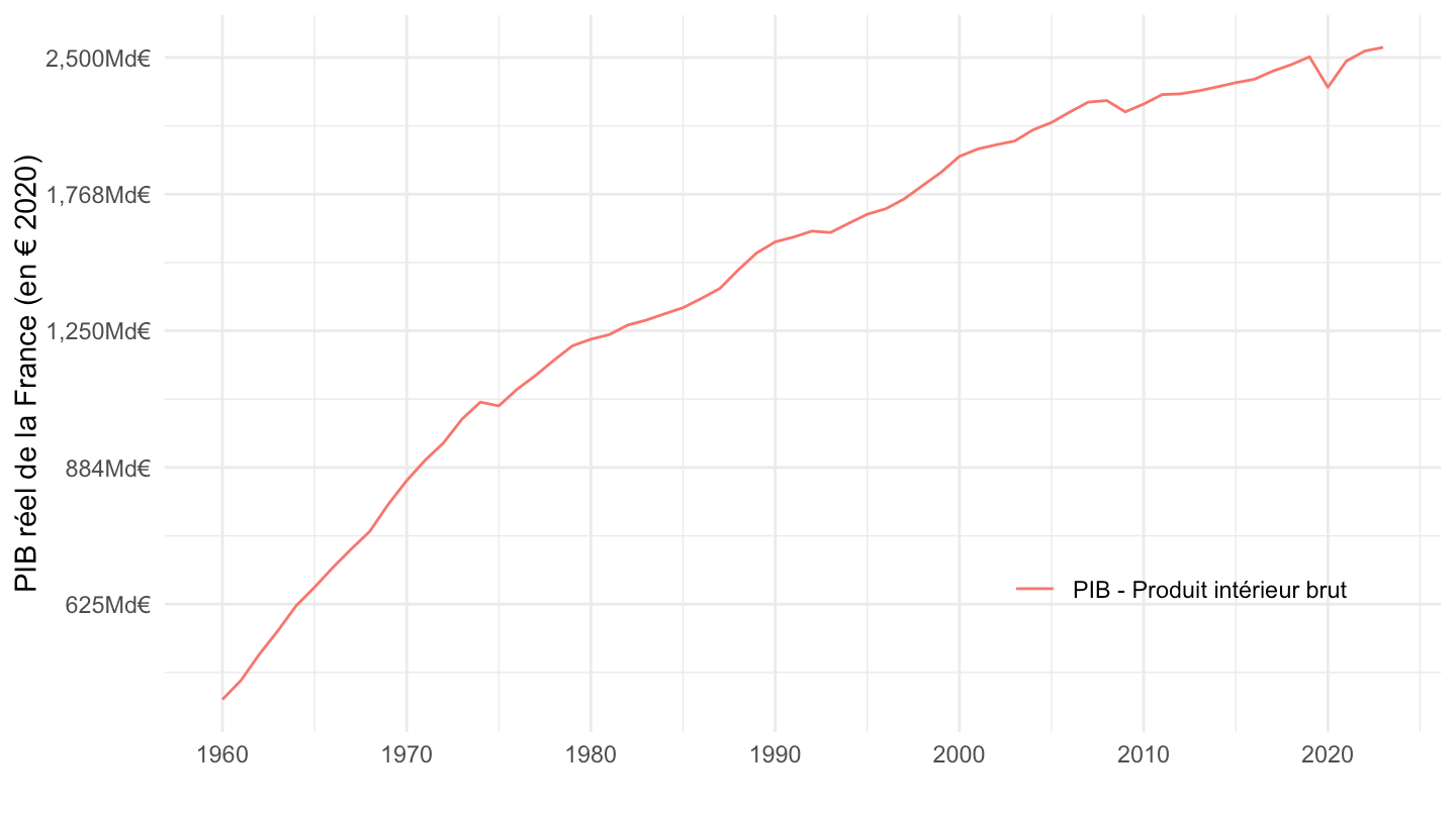
ggarrange(plot_lineaire + ggtitle("Echelle Linéaire"), plot_log + ggtitle("Echelle Log") + ylab(""), common.legend = T)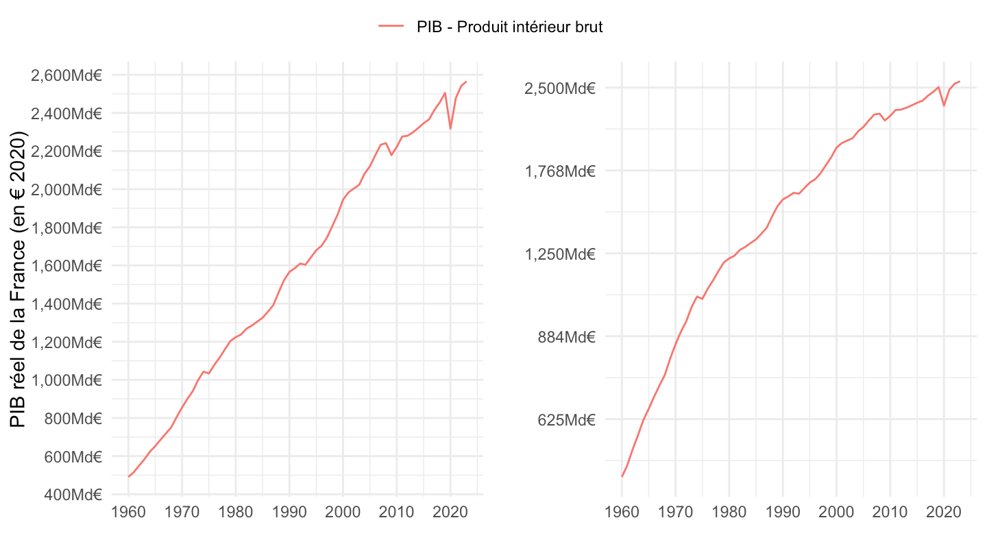
plot_lineaire <- `CNA-2020-PIB` |>
  filter(OPERATION %in% c("PIB", "P3"),
         UNIT_MEASURE == "EUR2020") |>

  year_to_date() |>
  mutate(year = year(date)) |>
  filter(year >= 2011,
         year <= 2013) |>
  arrange(date) |>
  mutate(OBS_VALUE = 100*OBS_VALUE/OBS_VALUE[1]) |>
  group_by(date) |>
  select(-year) |>
  ggplot() + theme_minimal() + xlab("") + ylab("PIB réel de la France (en € 2020)") +
  geom_line(aes(x = date, y = OBS_VALUE, color = Operation)) +
  scale_linetype_manual(values = c("solid", "solid", "dashed", "solid")) +
  theme(legend.title = element_blank(),
        legend.position = c(0.8, 0.2)) +
  scale_x_date(breaks = seq(1920, 2100, 1) |> paste0("-01-01") |> as.Date(),
               labels = date_format("%Y")) +
  scale_y_continuous(breaks = seq(100, 3000, 0.1))

plot_lineaire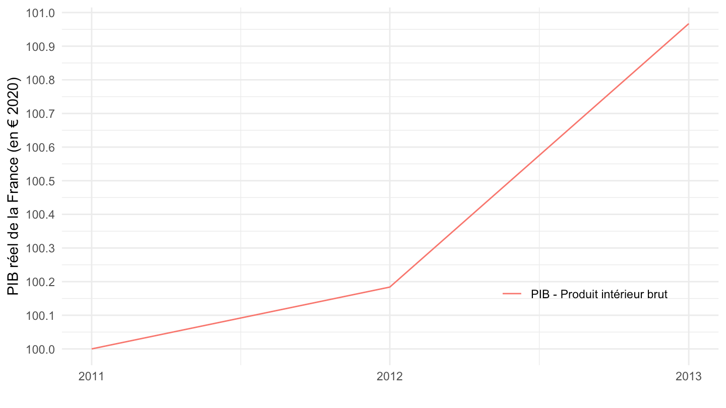
`CNA-2020-PIB` |>
  filter(OPERATION == "PIB",
         UNIT_MEASURE == "EUR2020") |>
  select(TIME_PERIOD, `PIB Réel` = OBS_VALUE) |>
  year_to_date() |>
  mutate(year = year(date)) |>
  filter(is.finite(`PIB Réel`)) |>
  mutate(`Tendance jusque 2024 (g = 2.9%)` = lm(log(`PIB Réel`) ~ year) |> fitted() |> exp()) |>
  group_by(date) |>
  select(-year) |>
  gather(variable, value, -date) |>
  ggplot() + theme_minimal() + xlab("") + ylab("PIB réel de la France (en € 2020)") +
  geom_line(aes(x = date, y = value/10^3, color = variable, linetype = variable)) +
  scale_linetype_manual(values = c("solid", "solid", "dashed", "solid")) +
  theme(legend.title = element_blank(),
        legend.position = c(0.8, 0.2)) +
  scale_x_date(breaks = seq(1920, 2100, 5) |> paste0("-01-01") |> as.Date(),
               labels = date_format("%Y")) +
  scale_y_log10(breaks = 20000*2^seq(-7, 1, 1),
                labels = scales::dollar_format(a = 1, prefix = "", suffix = "Md€"))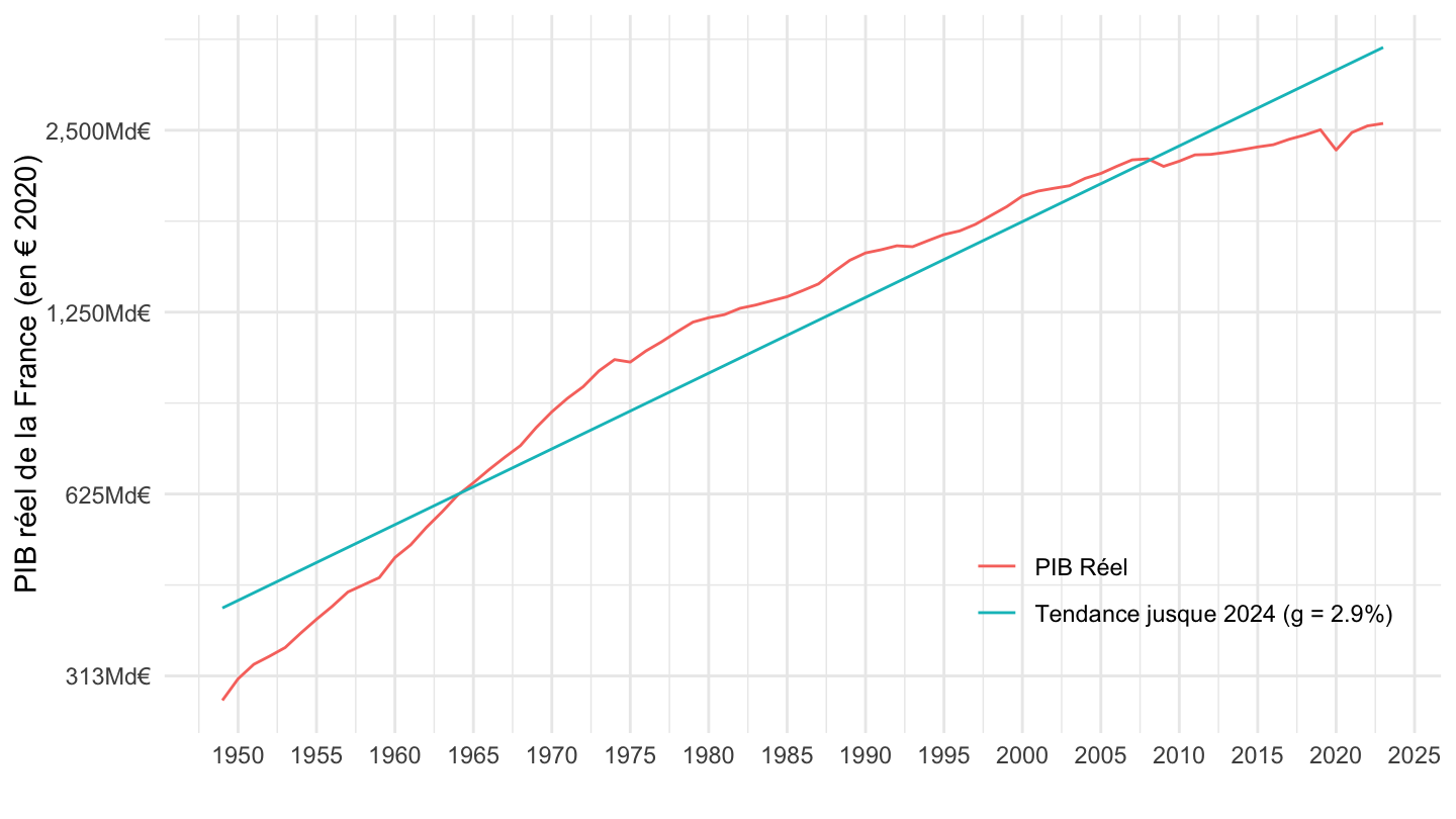
`CNA-2020-PIB` |>
  filter(OPERATION == "PIB",
         UNIT_MEASURE == "EUR2020") |>
  select(TIME_PERIOD, `PIB Réel` = OBS_VALUE) |>
  year_to_date() |>
  mutate(year = year(date)) |>
  filter(is.finite(`PIB Réel`)) |>
  mutate(`Tendance jusque 1971, extrapolée` = ifelse(year>=1971,
                                                (fit[1]+fit[2]*year) |> exp(),
                                                NA),
         `Tendance jusque 1971 (g = 5.1%)` = ifelse(year<=1971,
                                             (fit[1]+fit[2]*year) |> exp(),
                                             NA)) |>
  group_by(date) |>
  select(-year) |>
  gather(variable, value, -date) |>
  ggplot() + theme_minimal() + xlab("") + ylab("PIB réel de la France (en € 2020)") +
  geom_line(aes(x = date, y = value/10^3, color = variable, linetype = variable)) +
  scale_linetype_manual(values = c("solid", "solid", "dashed", "solid")) +
  theme(legend.title = element_blank(),
        legend.position = c(0.8, 0.2)) +
  scale_x_date(breaks = seq(1920, 2100, 5) |> paste0("-01-01") |> as.Date(),
               labels = date_format("%Y")) +
  scale_y_log10(breaks = 20000*2^seq(-7, 1, 1),
                labels = scales::dollar_format(a = 1, prefix = "", suffix = "Md€"))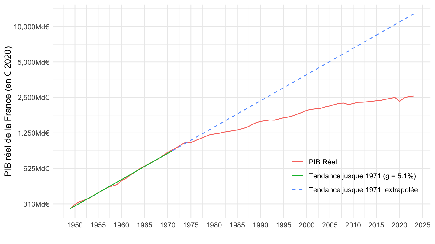
`CNA-2020-PIB` |>
  filter(OPERATION == "PIB",
         UNIT_MEASURE == "EUR2020") |>
  select(TIME_PERIOD, `PIB Réel` = OBS_VALUE) |>
  year_to_date() |>
  mutate(year = year(date)) |>
  filter(is.finite(`PIB Réel`)) |>
  mutate(`Tendance jusque 2024 (g = 2.9%)` = lm(log(`PIB Réel`) ~ year) |> fitted() |> exp(),
         `Tendance jusque 1971, extrapolée` = ifelse(year>=1971,
                                                (fit[1]+fit[2]*year) |> exp(),
                                                NA),
         `Tendance jusque 1971 (g = 5.1%)` = ifelse(year<=1971,
                                             (fit[1]+fit[2]*year) |> exp(),
                                             NA)) |>
  group_by(date) |>
  select(-year) |>
  gather(variable, value, -date) |>
  ggplot() + theme_minimal() + xlab("") + ylab("PIB réel de la France (en € 2020)") +
  geom_line(aes(x = date, y = value/10^3, color = variable, linetype = variable)) +
  scale_linetype_manual(values = c("solid", "solid", "dashed", "solid")) +
  theme(legend.title = element_blank(),
        legend.position = c(0.8, 0.2)) +
  scale_x_date(breaks = seq(1920, 2100, 5) |> paste0("-01-01") |> as.Date(),
               labels = date_format("%Y")) +
  scale_y_log10(breaks = 20000*2^seq(-7, 1, 1),
                labels = scales::dollar_format(a = 1, prefix = "", suffix = "Md€"))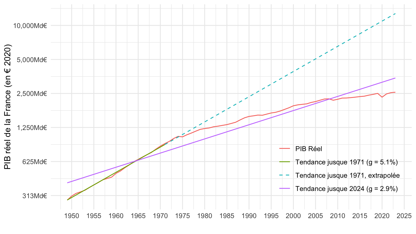
`CNA-2020-PIB` |>
  filter(OPERATION %in% c("P3", "P51G"),
         NATURE == "PROPORTION_POURCENTAGE",
         `SECT-INST` == "S0") |>
  year_to_date() |>
  select(OPERATION, OBS_VALUE, date) |>
  left_join(OPERATION,  by = "OPERATION") |>
  ggplot() + theme_minimal() + xlab("") + ylab("Contribution à la croissance du PIB") +
  geom_line(aes(x = date, y = OBS_VALUE/100, color = Operation)) +

  theme(legend.title = element_blank(),
        legend.position = c(0.7, 0.9)) +
  scale_x_date(breaks = seq(1920, 2100, 5) |> paste0("-01-01") |> as.Date(),
               labels = date_format("%Y")) +
  scale_y_continuous(breaks = 0.01*seq(-200, 200, 1),
                     labels = scales::percent_format(accuracy = 1)) +
  geom_hline(yintercept = 0, linetype = "dashed")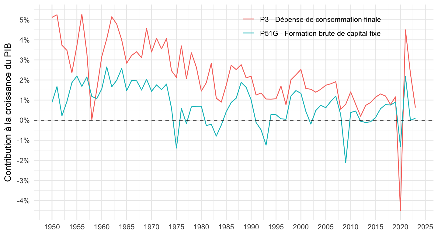
`CNA-2020-PIB` |>
  filter(OPERATION %in% c("P6", "P7"),
         NATURE == "PROPORTION_POURCENTAGE",
         `SECT-INST` == "S0") |>
  year_to_date() |>
  select(OPERATION, OBS_VALUE, date) |>
  left_join(OPERATION,  by = "OPERATION") |>
  ggplot() + theme_minimal() + xlab("") + ylab("") +
  geom_line(aes(x = date, y = OBS_VALUE/100, color = Operation)) +

  theme(legend.title = element_blank(),
        legend.position = c(0.8, 0.2)) +
  scale_x_date(breaks = seq(1920, 2100, 5) |> paste0("-01-01") |> as.Date(),
               labels = date_format("%Y")) +
  scale_y_continuous(breaks = 0.01*seq(-200, 200, 1),
                     labels = scales::percent_format(accuracy = 1)) +
  geom_hline(yintercept = 0, linetype = "dashed")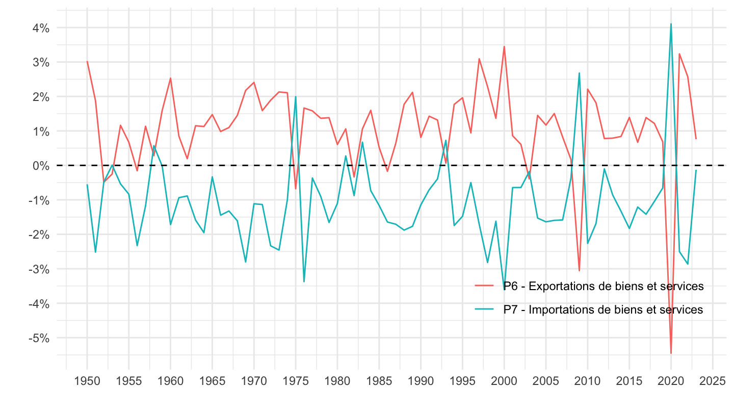
`CNA-2020-PIB` |>
  filter(OPERATION %in% c("B11", "P6", "P7"),
         NATURE == "PROPORTION_POURCENTAGE",
         `SECT-INST` == "S0") |>
  year_to_date() |>
  select(OPERATION, OBS_VALUE, date) |>
  left_join(OPERATION,  by = "OPERATION") |>
  ggplot() + theme_minimal() + xlab("") + ylab("") +
  geom_line(aes(x = date, y = OBS_VALUE/100, color = Operation)) +

  theme(legend.title = element_blank(),
        legend.position = c(0.7, 0.2)) +
  scale_x_date(breaks = seq(1920, 2100, 5) |> paste0("-01-01") |> as.Date(),
               labels = date_format("%Y")) +
  scale_y_continuous(breaks = 0.01*seq(-200, 200, 1),
                     labels = scales::percent_format(accuracy = 1)) +
  geom_hline(yintercept = 0, linetype = "dashed")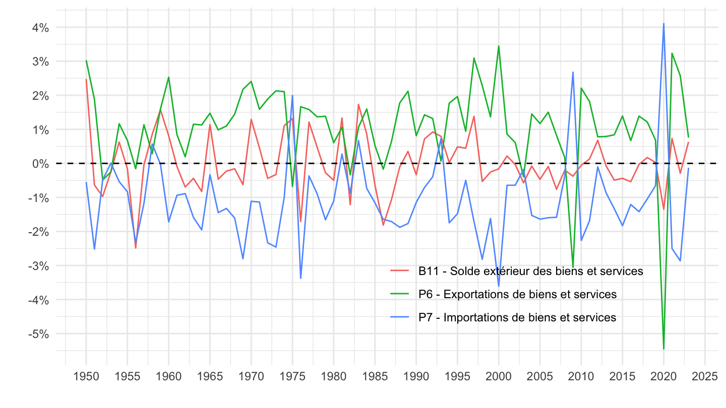
| source | dataset | Title | Updated |
|---|---|---|---|

