Code
i_g("bib/insee/FPORSOC22/F29/table2.png")
Data - INSEE
i_g("bib/insee/FPORSOC22/F29/table2.png")
i_g("bib/insee/FPS2021/revenu-primaire-RDB.png")
t_2101 %>%
  group_by(line, variable, Variable) %>%
  summarise(Nobs = n()) %>%
print_table_conditional| line | variable | Variable | Nobs |
|---|---|---|---|
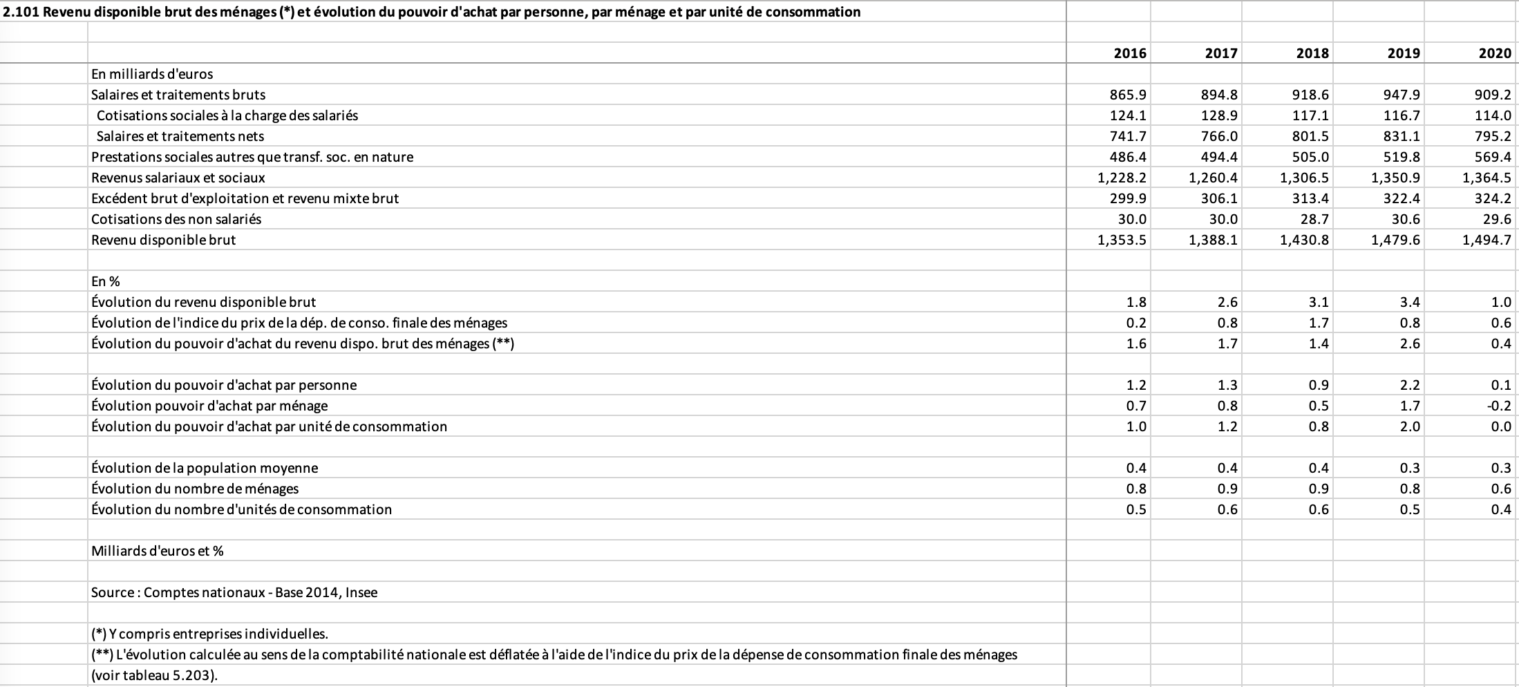
| 1 | D11 | Salaires et traitements bruts | 64 |
| 2 | D613CE | Cotisations sociales effectives obligatoires à la charge des salariés | 64 |
| 3 | D11X613CE | Salaires et traitements nets | 64 |
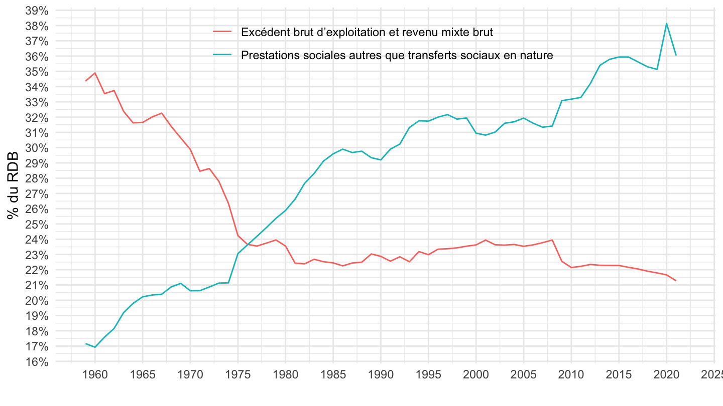
| 4 | D62 | Prestations sociales autres que transferts sociaux en nature | 64 |
| 5 | RSS | Revenus salariaux et sociaux | 64 |
| 6 | B2A3G | Excédent brut d’exploitation et revenu mixte brut | 64 |
| 7 | D613NSI | Cotisations des non salariés | 64 |
| 8 | B6G | Revenu disponible brut | 64 |
| 9 | B6G | Revenu disponible brut | 64 |
| 10 | P31 | Dépense de consommation individuelle | 64 |
| 11 | _PAM | Pouvoir d’achat du rdb des ménages (**) | 63 |
| 12 | _PAM_PERSONNE | Pouvoir d’achat du rdb par personne | 63 |
| 13 | _PAM_MENAGE | Pouvoir d’achat du rdb par ménage | 63 |
| 14 | _PAM_UC | Pouvoir d’achat du rdb par unité de consommation | 63 |
| 15 | POP | Population | 64 |
| 16 | MENF | Moyenne annuelle du nombre de ménages en France entière | 63 |
| 17 | UC | Unités de consommation | 63 |
t_2101 %>%
  filter(line %in% c(1, 3)) %>%
  left_join(gdp, by = "year") %>%
  year_to_date2 %>%
  ggplot + geom_line(aes(x = date, y = value / gdp, color = Variable)) +
  theme_minimal() + xlab("") + ylab("% du PIB") +
  scale_x_date(breaks ="5 years",
               labels = date_format("%Y")) +
  scale_y_continuous(breaks = 0.01*seq(-10, 100, 1),
                     labels = percent_format(accuracy = 1)) +
  theme(legend.position = c(0.2, 0.15),
        legend.title = element_blank())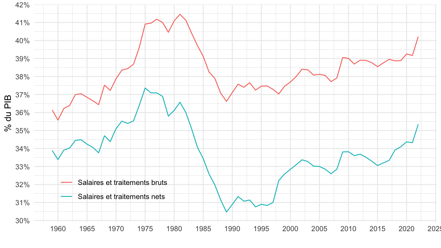
t_2101 %>%
  filter(line %in% c(1, 3)) %>%
  left_join(rdb, by = "year") %>%
  year_to_date2 %>%
  ggplot + geom_line(aes(x = date, y = value / rdb, color = Variable)) +
  theme_minimal() + xlab("") + ylab("% du RDB") +
  scale_x_date(breaks ="5 years",
               labels = date_format("%Y")) +
  scale_y_continuous(breaks = 0.01*seq(-10, 100, 1),
                     labels = percent_format(accuracy = 1)) +
  theme(legend.position = c(0.15, 0.93),
        legend.title = element_blank())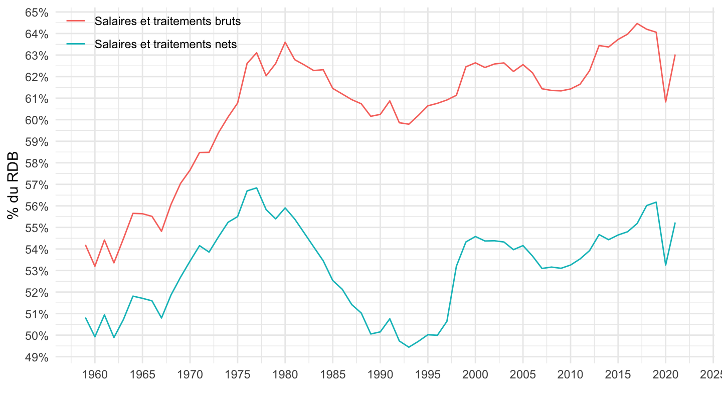
t_2101 %>%
  filter(line %in% c(4, 6)) %>%
  left_join(gdp, by = "year") %>%
  year_to_date2 %>%
  ggplot + geom_line(aes(x = date, y = value / gdp, color = Variable)) +
  theme_minimal() + xlab("") + ylab("% du PIB") +
  scale_x_date(breaks ="5 years",
               labels = date_format("%Y")) +
  scale_y_continuous(breaks = 0.01*seq(-10, 100, 1),
                     labels = percent_format(accuracy = 1)) +
  theme(legend.position = c(0.5, 0.9),
        legend.title = element_blank())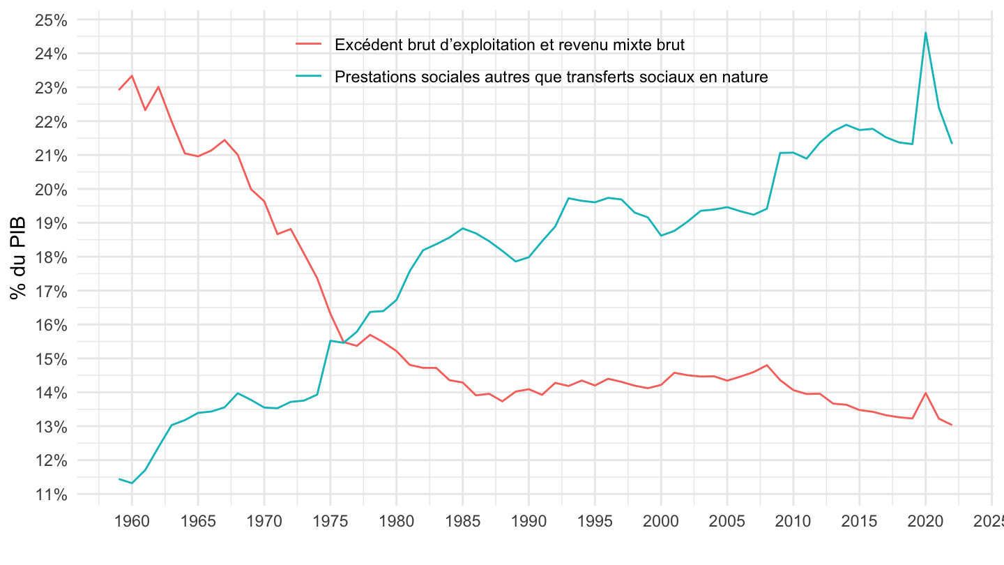
t_2101 %>%
  filter(line %in% c(4, 6)) %>%
  left_join(rdb, by = "year") %>%
  year_to_date2 %>%
  ggplot + geom_line(aes(x = date, y = value / rdb, color = Variable)) +
  theme_minimal() + xlab("") + ylab("% du RDB") +
  scale_x_date(breaks ="5 years",
               labels = date_format("%Y")) +
  scale_y_continuous(breaks = 0.01*seq(-10, 100, 1),
                     labels = percent_format(accuracy = 1)) +
  theme(legend.position = c(0.5, 0.9),
        legend.title = element_blank())