1.101 – Le produit intérieur brut et ses composantes à prix courants (En milliards d’euros)

Data - INSEE

Info

  • Comptes de la Nation 2021. html

  • Comptes de la Nation 2020. html

  • Comptes de la Nation 2019. html

2020

Désordonné

Code
t_1101 %>%
  left_join(gdp, by = "date") %>%
  filter(date == as.Date("2020-01-01")) %>%
  select(-date) %>%
  mutate(`% du PIB` = (100*value/gdp) %>% round(., digits = 2) %>% paste0(., " %"),
         value = round(value) %>% paste0(" Mds€")) %>%
  select(-gdp) %>%
  {if (is_html_output()) datatable(., filter = 'top', rownames = F) else .}

Ordre

Code
t_1101 %>%
  left_join(gdp, by = "date") %>%
  filter(date == as.Date("2020-01-01")) %>%
  select(-date) %>%
  arrange(-value) %>%
  mutate(`% du PIB` = (100*value/gdp) %>% round(., digits = 2) %>% paste0(., " %"),
         value = round(value) %>% paste0(" Mds€")) %>%
  select(-gdp) %>%
  {if (is_html_output()) datatable(., filter = 'top', rownames = F) else .}

2019

Désordonné

Code
t_1101 %>%
  left_join(gdp, by = "date") %>%
  filter(date == as.Date("2019-01-01")) %>%
  select(-date) %>%
  mutate(`% du PIB` = (100*value/gdp) %>% round(., digits = 2) %>% paste0(., " %"),
         value = round(value) %>% paste0(" Mds€")) %>%
  select(-gdp) %>%
  {if (is_html_output()) datatable(., filter = 'top', rownames = F) else .}

Ordre

Code
t_1101 %>%
  left_join(gdp, by = "date") %>%
  filter(date == as.Date("2019-01-01")) %>%
  select(-date) %>%
  arrange(-value) %>%
  mutate(`% du PIB` = (100*value/gdp) %>% round(., digits = 2) %>% paste0(., " %"),
         value = round(value) %>% paste0(" Mds€")) %>%
  select(-gdp) %>%
  {if (is_html_output()) datatable(., filter = 'top', rownames = F) else .}

Administration publique: Dépenses collective et individuelle

Code
t_1101 %>%
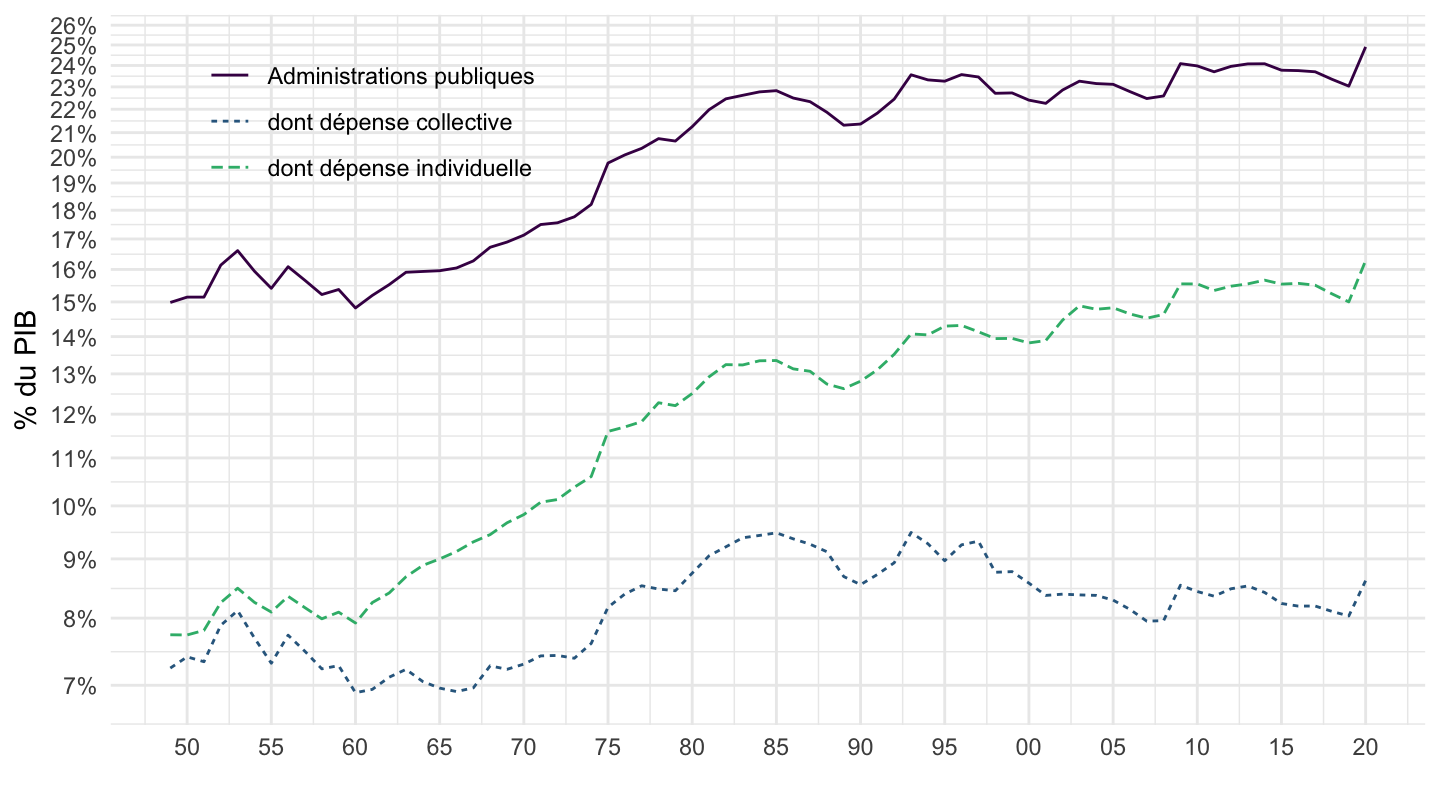
  filter(line %in% c(8, 10, 9)) %>%
  left_join(gdp, by = "date") %>%
  ggplot(.) + theme_minimal() + ylab("% du PIB") + xlab("") +
  geom_line(aes(x = date, y = value/gdp, color = Line, linetype = Line)) +
  theme(legend.title = element_blank(),
        legend.position = c(0.2, 0.85)) +
  scale_x_date(breaks = seq(1950, 2020, 5) %>% paste0("-01-01") %>% as.Date,
               labels = date_format("%y")) +
  scale_color_manual(values = viridis(4)[1:3]) +
  scale_y_log10(breaks = 0.01*seq(0, 100, 1),
                     labels = scales::percent_format(accuracy = 1))

GDP Components

Code
t_1101 %>%
  filter(line %in% c(8, 12, 9)) %>%
  left_join(gdp, by = "date") %>%
  ggplot(.) + theme_minimal() + ylab("% du PIB") + xlab("") +
  geom_line(aes(x = date, y = value/gdp, color = Line, linetype = Line)) +
  theme(legend.title = element_blank(),
        legend.position = c(0.7, 0.15)) +
  scale_x_date(breaks = seq(1950, 2020, 5) %>% paste0("-01-01") %>% as.Date,
               labels = date_format("%y")) +
  scale_color_manual(values = viridis(4)[1:3]) +
  scale_y_log10(breaks = 0.01*seq(0, 100, 1),
                     labels = scales::percent_format(accuracy = 1))

Investissement et taux de marge

Code
t_1101 %>%
  filter(line %in% c(12)) %>%
  left_join(gdp, by = "date") %>%
  mutate(value = value/gdp) %>%
  select(Variable = Line, date, value) %>%
  mutate(Variable = "Investissement (% du PIB)") %>%
  bind_rows(t_txmargesnf_val %>%
              filter(variable == "taux_marge") %>%
              mutate(Variable = "Taux de marge") %>%
              mutate(value = value/100)) %>%
  ggplot(.) + theme_minimal() + ylab("") + xlab("") +
  geom_line(aes(x = date, y = value, color = Variable)) +
  theme(legend.title = element_blank(),
        legend.position = c(0.3, 0.9)) +
  scale_x_date(breaks = seq(1950, 2020, 5) %>% paste0("-01-01") %>% as.Date,
               labels = date_format("%y")) +
  scale_color_manual(values = viridis(3)[1:2]) +
  scale_y_continuous(breaks = 0.01*seq(0, 100, 1),
                     labels = scales::percent_format(accuracy = 1))