Comptes Financiers Trimestriels

Data - BDF

Author

Info

source	dataset	Title	.html	.rData
bdf	CFT	Comptes Financiers Trimestriels	2025-12-20	2025-03-09

Méthodologie. pdf

Last

date	Nobs
2024-09-30	4

Liste des publications

Épargne et Patrimoine financiers des ménages, 2024T1. pdf / html
Comptes financiers des agents non financiers. STAT INFO – 4e trimestre 2023. pdf
Épargne des ménages. STAT INFO – février 2024. pdf

Info

Épargne et Patrimoine financiers des ménages, 2024T2. pdf html
Épargne et Patrimoine financiers des ménages, Comptes financiers des agents non financiers, 15 avril 2024, 2023T4. pdf html
Épargne et Patrimoine financiers des ménages, 2023T3. pdf
Épargne et Patrimoine financiers des ménages, 2023T2. pdf
Présentation trimestrielle de l’épargne des ménages, 2023T1. html pdf
Méthodologie. pdf
Liste séries. html
Épargne et Patrimoine financiers des ménages, 2022T2. pdf
Epargne des ménages, 2021T1. pdf
Taux d’endettement des agents non financiers – Comparaisons internationales, 2020T4. html / pdf
Epargne des ménages, 2020T3. pdf

STO

Code

CFT %>%
  left_join(CFT_var, by = "variable") %>%
  left_join(STO, by = "STO") %>%
  group_by(STO, Sto) %>%
  summarise(Nobs = n()) %>%
  arrange(-Nobs) %>%
  print_table_conditional

STO	Sto	Nobs
F	flux	13459
LE	Encours	8793
B8G	Taux d'épargne des ménages	836
B9Z	Taux d'épargne financière des ménages	693
K	Réévaluations et autres changements de volume	258
K5	Impact de valorisation	167
P51G	Formation brute de capital fixe	143

FREQ Frequency

Code

CFT %>%
  left_join(CFT_var, by = "variable") %>%
  left_join(FREQ, by = "FREQ") %>%
  group_by(FREQ, Freq) %>%
  summarise(Nobs = n()) %>%
  arrange(-Nobs) %>%
  print_table_conditional

FREQ	Freq	Nobs
Q	Trimestriel	22870
A	Annuel	1479

ADJUSTMENT Adjustment

Code

CFT %>%
  left_join(CFT_var, by = "variable") %>%
  left_join(ADJUSTMENT, by = "ADJUSTMENT") %>%
  group_by(ADJUSTMENT, Adjustment) %>%
  summarise(Nobs = n()) %>%
  arrange(-Nobs) %>%
  print_table_conditional

ADJUSTMENT	Adjustment	Nobs
N	Brut	11931
S	CVS	11874
Y	CVS/CJO	286
_Z	Non applicable	258

REF_AREA Reference area - ISO2

Code

CFT %>%
  left_join(CFT_var, by = "variable") %>%
  left_join(REF_AREA, by = "REF_AREA") %>%
  group_by(REF_AREA, Ref_area) %>%
  summarise(Nobs = n()) %>%
  arrange(-Nobs) %>%
  print_table_conditional

REF_AREA	Ref_area	Nobs
FR	France	18452
DE	Germany	936
ES	Spain	936
IT	Italy	936
US	United States	936
GB	United Kingdom	831
I9	NA	710
JP	Japan	612

COUNTERPART_AREA Counterpart area

Code

CFT %>%
  left_join(CFT_var, by = "variable") %>%
  left_join(COUNTERPART_AREA, by = "COUNTERPART_AREA") %>%
  group_by(COUNTERPART_AREA, Counterpart_area) %>%
  summarise(Nobs = n()) %>%
  arrange(-Nobs) %>%
  print_table_conditional

COUNTERPART_AREA	Counterpart_area	Nobs
W0	World (all areas, including reference area, including IO)	23314
W2	Domestic (home or reference area)	1035

REF_SECTOR Reference sector

Code

CFT %>%
  left_join(CFT_var, by = "variable") %>%
  left_join(REF_SECTOR, by = "REF_SECTOR") %>%
  group_by(REF_SECTOR, Ref_sector) %>%
  summarise(Nobs = n()) %>%
  arrange(-Nobs) %>%
  print_table_conditional

REF_SECTOR	Ref_sector	Nobs
S1M	Ménages et Institution sans but lucratif au service des ménages (ISBLSM)	14519
S11	Sociétés non financières	5326
S13	Administrations publiques	3586
S1V	Sociétés non-financières, ménages et NPISH	918

COUNTERPART_SECTOR Counterpart sector

Code

CFT %>%
  left_join(CFT_var, by = "variable") %>%
  left_join(COUNTERPART_SECTOR, by = "COUNTERPART_SECTOR") %>%
  group_by(COUNTERPART_SECTOR, Counterpart_sector) %>%
  summarise(Nobs = n()) %>%
  arrange(-Nobs) %>%
  print_table_conditional

COUNTERPART_SECTOR	Counterpart_sector	Nobs
S1	Ensemble de l`économie	23314
S124	des OPC non monétaires	1035

ACCOUNTING_ENTRY Accounting entries

Code

CFT %>%
  left_join(CFT_var, by = "variable") %>%
  left_join(ACCOUNTING_ENTRY, by = "ACCOUNTING_ENTRY") %>%
  group_by(ACCOUNTING_ENTRY, Accounting_entry) %>%
  summarise(Nobs = n()) %>%
  arrange(-Nobs) %>%
  print_table_conditional

ACCOUNTING_ENTRY	Accounting_entry	Nobs
A	Créances	13245
L	Engagements	8673
B	Balance (Crédit moins débit)	1529
N	Net (avoirs moins engagements)	506
NE	Engagements Nets (engagements moins avoirs)	253
D	Débit (dépenses)	143

INSTR_ASSET Instrument and assets classification

Code

CFT %>%
  left_join(CFT_var, by = "variable") %>%
  left_join(INSTR_ASSET, by = "INSTR_ASSET") %>%
  group_by(INSTR_ASSET, Instr_asset) %>%
  summarise(Nobs = n()) %>%
  #arrange(-Nobs) %>%
  print_table_conditional

MATURITY Maturity

Code

CFT %>%
  left_join(CFT_var, by = "variable") %>%
  left_join(MATURITY, by = "MATURITY") %>%
  group_by(MATURITY, Maturity) %>%
  summarise(Nobs = n()) %>%
  arrange(-Nobs) %>%
  print_table_conditional

MATURITY	Maturity	Nobs
T	Toutes maturités d`origine	12536
_Z	Non applicable	11813

UNIT_MEASURE Unit of measure

Code

CFT %>%
  left_join(CFT_var, by = "variable") %>%
  left_join(UNIT_MEASURE, by = "UNIT_MEASURE") %>%
  group_by(UNIT_MEASURE, Unit_measure) %>%
  summarise(Nobs = n()) %>%
  arrange(-Nobs) %>%
  print_table_conditional

UNIT_MEASURE	Unit_measure	Nobs
XDC	Monnaie nationale	17073
XDC_R_B1GQ_CY	Monnaie nationale (incl. une conversion à la monnaie courante en utilisant une parité fixe); ratio à la somme du glissement annuel du produit intérieur brut	3260
XDC_R_B6G_S1M	en % du RDB	2202
XDC_R_B1G_CY	NA	809
XDC_R_DEBT	NA	612
PC	Pourcent	393

CURRENCY_DENOM Currency denominator

Code

CFT %>%
  left_join(CFT_var, by = "variable") %>%
  left_join(CURRENCY_DENOM, by = "CURRENCY_DENOM") %>%
  group_by(CURRENCY_DENOM, Currency_denom) %>%
  summarise(Nobs = n()) %>%
  arrange(-Nobs) %>%
  print_table_conditional

CURRENCY_DENOM	Currency_denom	Nobs
_T	Toutes monnaies d`opération	24349

VALUATION Valuation

Code

CFT %>%
  left_join(CFT_var, by = "variable") %>%
  left_join(VALUATION, by = "VALUATION") %>%
  group_by(VALUATION, Valuation) %>%
  summarise(Nobs = n()) %>%
  arrange(-Nobs) %>%
  print_table_conditional

VALUATION	Valuation	Nobs
S	Valorisation standard basée sur ESA2010/SNA2008	23129
N	Valeur nominale (N)	612
F	Valeur nominale (F)	608

date

Code

CFT %>%
  group_by(date) %>%
  summarise(Nobs = n()) %>%
  arrange(desc(date)) %>%
  print_table_conditional

Grandes masses

2024T2

Code

ig_b("bdf", "CFT-2024T2")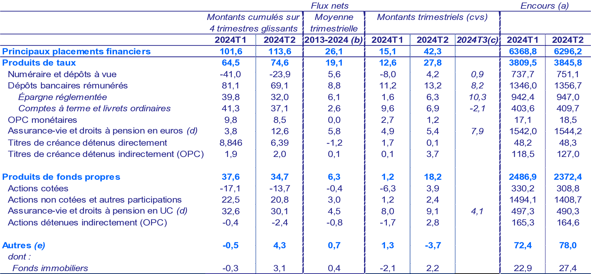

2023T4

Code

ig_b("bdf", "CFT-2023T4")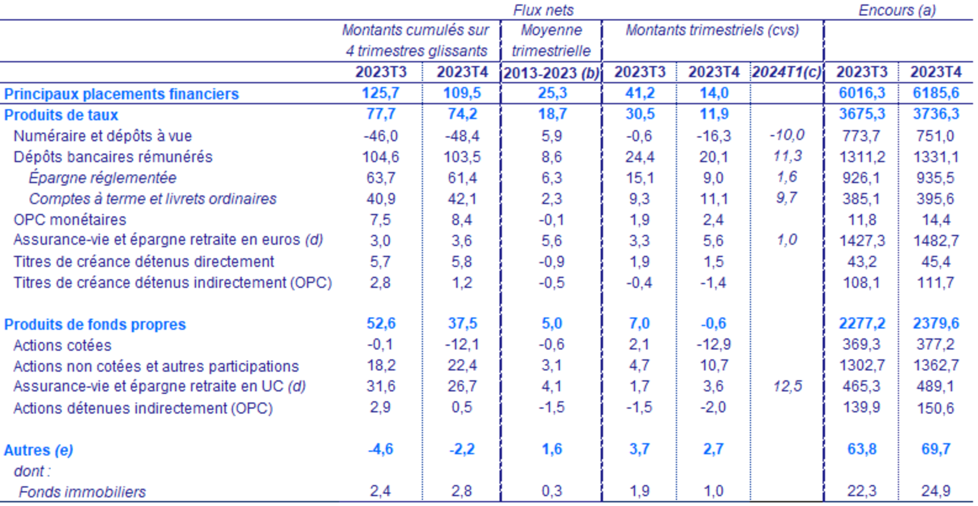

Produits de taux

Code

CFT %>%
  left_join(CFT_var, by = "variable") %>%
  filter(STO == "LE",
         INSTR_ASSET %in% c("PDTX")) %>%
  na.omit %>%
  ggplot + geom_line(aes(x = date, y = value, color = Variable)) + 
  xlab("") + ylab("") + theme_minimal() +
  scale_x_date(breaks = "1 year",
               labels = date_format("%Y")) +
  scale_y_log10(breaks = seq(-200, 10000, 100),
                     labels = dollar_format(acc = 1, prefix = "", su = "Mds€")) +
  theme(legend.position = c(0.35, 0.9),
        legend.title = element_blank(),
        legend.direction = "vertical") +
  geom_label(data = . %>% filter(date == as.Date("2023-12-31")),
             aes(x = date, y = value, color = Variable, label = round(value)))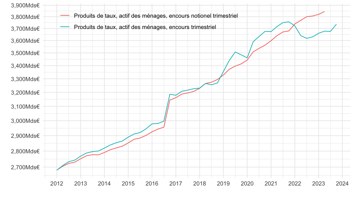

Produits de fonds propres

Code

CFT %>%
  left_join(CFT_var, by = "variable") %>%
  filter(STO == "LE",
         INSTR_ASSET %in% c("PDFP")) %>%
  na.omit %>%
  ggplot + geom_line(aes(x = date, y = value, color = Variable)) + 
  xlab("") + ylab("") + theme_minimal() +
  scale_x_date(breaks = "1 year",
               labels = date_format("%Y")) +
  scale_y_log10(breaks = seq(-200, 10000, 100),
                     labels = dollar_format(acc = 1, prefix = "", su = "Mds€")) +
  theme(legend.position = c(0.35, 0.9),
        legend.title = element_blank(),
        legend.direction = "vertical") +
  geom_label(data = . %>% filter(date == as.Date("2023-12-31")),
             aes(x = date, y = value, color = Variable, label = round(value)))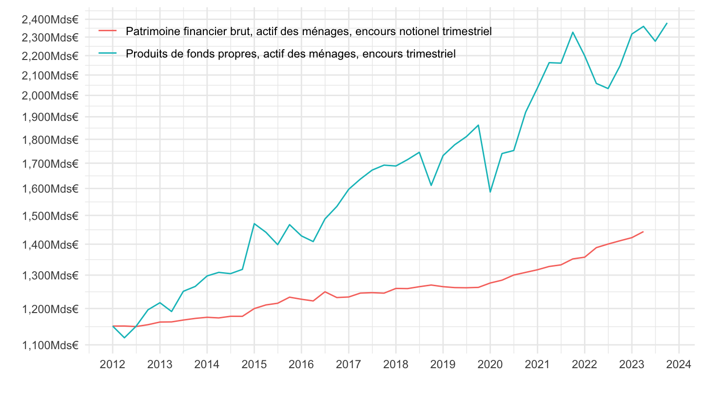

Côté, non côté

Code

CFT %>%
  left_join(CFT_var, by = "variable") %>%
  filter(STO == "LE",
         INSTR_ASSET %in% c("PDFP", "F51", "F511", "F51M", "F52")) %>%
  na.omit %>%
  ggplot + geom_line(aes(x = date, y = value, color = Variable)) + 
  xlab("") + ylab("") + theme_minimal() +
  scale_x_date(breaks = "1 year",
               labels = date_format("%Y")) +
  scale_y_log10(breaks = seq(-200, 10000, 100),
                     labels = dollar_format(acc = 1, prefix = "", su = "Mds€")) +
  theme(legend.position = c(0.5, 0.7),
        legend.title = element_blank(),
        legend.direction = "vertical") +
  geom_label(data = . %>% filter(date == as.Date("2023-12-31")),
             aes(x = date, y = value, color = Variable, label = round(value)))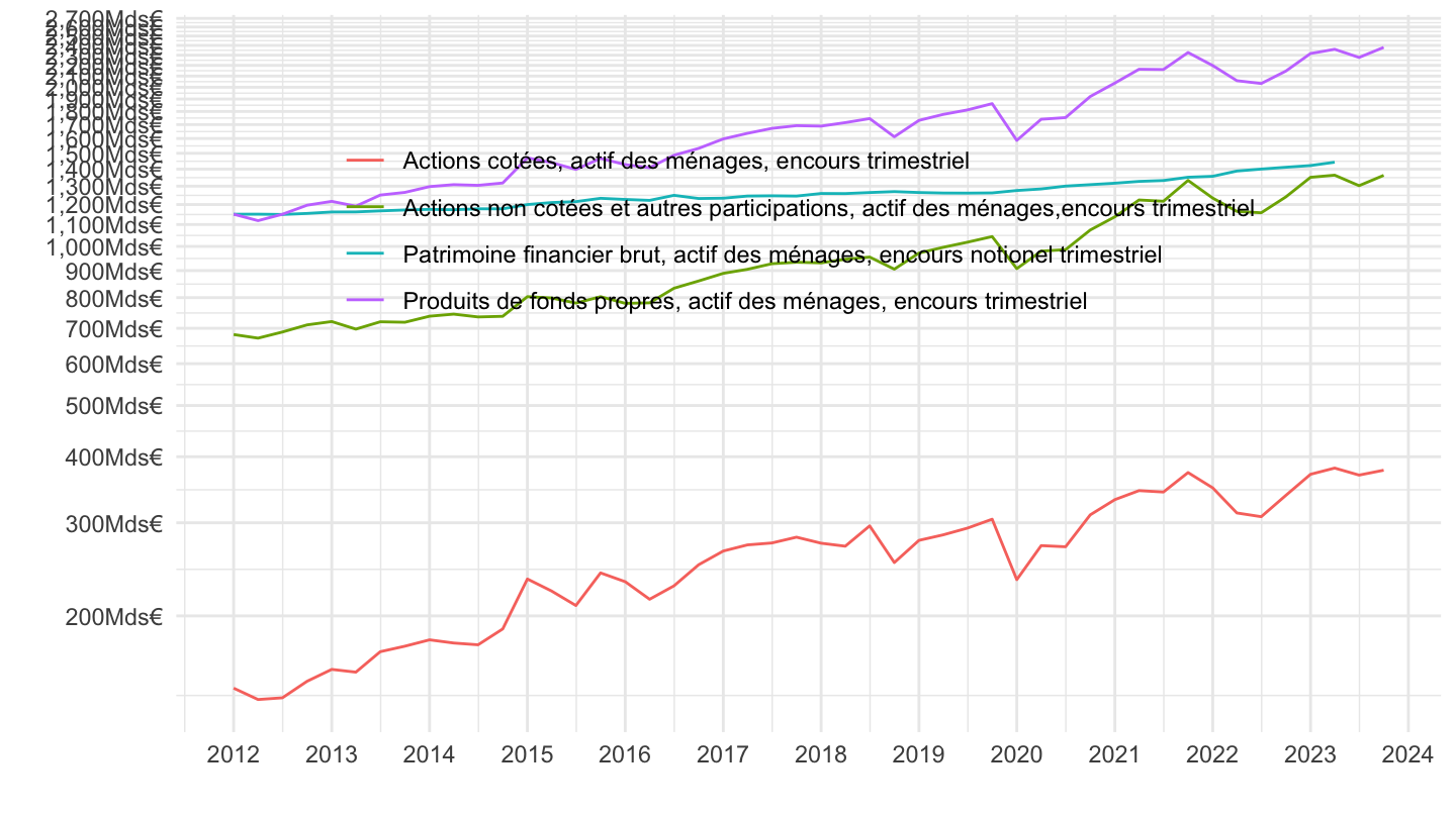

Detail

Linéaire

Code

CFT %>%
  left_join(CFT_var, by = "variable") %>%
  filter(STO == "LE",
         INSTR_ASSET %in% c("F62A", "F62B", "F29R", "F2A", "F29Z")) %>%
  na.omit %>%
  ggplot + geom_line(aes(x = date, y = value, color = Variable)) + 
  xlab("") + ylab("") + theme_minimal() +
  scale_x_date(breaks = "1 year",
               labels = date_format("%Y")) +
  scale_y_continuous(breaks = seq(-200, 10000, 100),
                     labels = dollar_format(acc = 1, prefix = "", su = "Mds€")) +
  theme(legend.position = c(0.45, 0.17),
        legend.title = element_blank(),
        legend.direction = "vertical") +
  geom_label(data = . %>% filter(date == as.Date("2023-12-31")),
             aes(x = date, y = value, color = Variable, label = round(value)))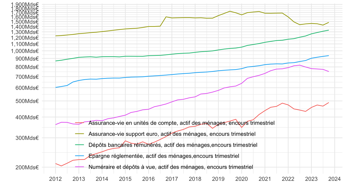

Log

Code

CFT %>%
  left_join(CFT_var, by = "variable") %>%
  filter(STO == "LE",
         INSTR_ASSET %in% c("F62A", "F62B", "F29R", "F2A", "F29Z")) %>%
  na.omit %>%
  ggplot + geom_line(aes(x = date, y = value, color = Variable)) + 
  xlab("") + ylab("") + theme_minimal() +
  scale_x_date(breaks = "1 year",
               labels = date_format("%Y")) +
  scale_y_log10(breaks = seq(-200, 10000, 100),
                     labels = dollar_format(acc = 1, prefix = "", su = "Mds€")) +
  theme(legend.position = c(0.45, 0.17),
        legend.title = element_blank(),
        legend.direction = "vertical") +
  geom_label(data = . %>% filter(date == as.Date("2023-12-31")),
             aes(x = date, y = value, color = Variable, label = round(value)))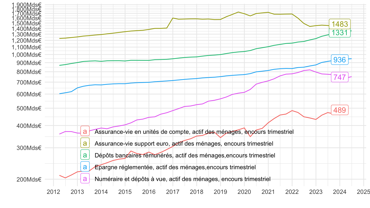

Stock

Numéraires et dépôts à vue

Code

CFT %>%
  left_join(CFT_var, by = "variable") %>%
  left_join(REF_AREA, by = "REF_AREA") %>%
  filter(REF_AREA %in% c("FR", "IT", "DE"),
         INSTR_ASSET == "F2A",
         STO == "LE") %>%
  mutate(Ref_area = ifelse(REF_AREA == "I8", "Europe", Ref_area)) %>%
  left_join(colors, by = c("Ref_area" = "country")) %>%
  na.omit %>%
  ggplot + geom_line(aes(x = date, y = value, color = color)) + 
  xlab("") + ylab("") + theme_minimal() + scale_color_identity() + add_3flags +
  scale_x_date(breaks = "1 year",
               labels = date_format("%Y")) +
  scale_y_log10(breaks = seq(100, 4000, 100),
                labels = dollar_format(accuracy = 1, pre = "", su = " Mds€")) +
  geom_label(data = . %>% filter(date == as.Date("2023-12-31")),
             aes(x = date, y = value, label = round(value)))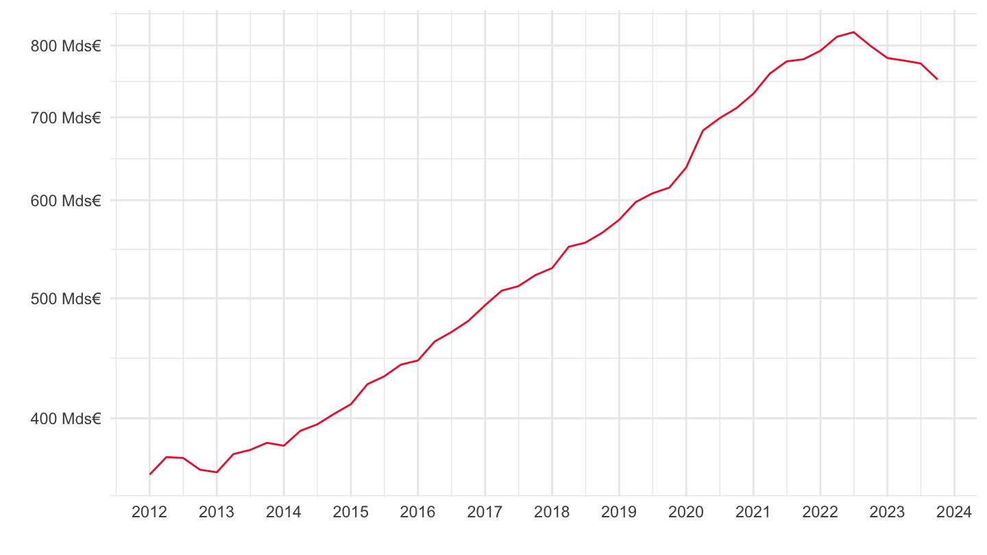

Stocks

Code

CFT %>%
  left_join(CFT_var, by = "variable") %>%
  left_join(INSTR_ASSET, by = "INSTR_ASSET") %>%
  filter(REF_AREA %in% c("FR"),
         INSTR_ASSET %in% c("F2A", "F29Z", "F62B", "F29R"),
         STO == "LE") %>%
  select(date, value, Instr_asset) %>%
  na.omit %>%
  ggplot + geom_line(aes(x = date, y = value, color = Instr_asset)) + 
  xlab("") + ylab("") + theme_minimal() +
  
  scale_x_date(breaks = "1 year",
               labels = date_format("%Y")) +
  scale_y_log10(breaks = seq(100, 4000, 100),
                labels = dollar_format(accuracy = 1, pre = "", su = " Mds€")) +
  theme(legend.position = c(0.4, 0.4),
        legend.title = element_blank(),
        legend.direction = "vertical") +
  geom_label(data = . %>% filter(date == as.Date("2023-12-31")),
             aes(x = date, y = value, color = Instr_asset, label = round(value)))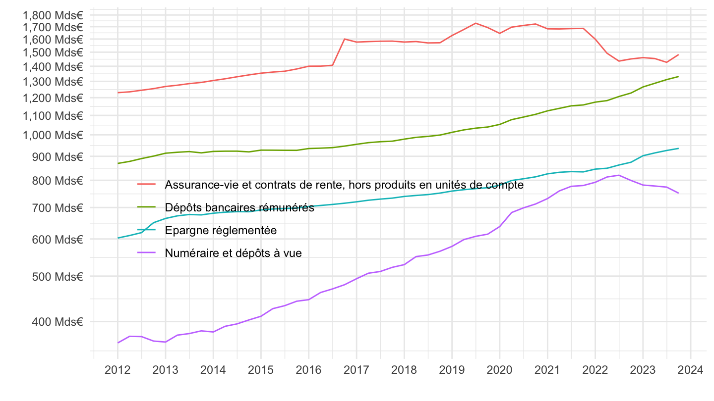

Numéraires et dépôts à vue

Stocks

All

Code

CFT %>%
  left_join(CFT_var, by = "variable") %>%
  left_join(INSTR_ASSET, by = "INSTR_ASSET") %>%
  filter(REF_AREA %in% c("FR"),
         INSTR_ASSET %in% c("F2A", "F29Z", "F62B"),
         STO == "LE") %>%
  select(date, value, Instr_asset) %>%
  na.omit %>%
  ggplot + geom_line(aes(x = date, y = value, color = Instr_asset)) + 
  xlab("") + ylab("") + theme_minimal() +
  
  scale_x_date(breaks = "1 year",
               labels = date_format("%Y")) +
  scale_y_log10(breaks = seq(100, 4000, 100),
                labels = dollar_format(accuracy = 1, pre = "", su = " Mds€")) +
  theme(legend.position = c(0.4, 0.4),
        legend.title = element_blank(),
        legend.direction = "vertical") +
  geom_label(data = . %>% filter(date == as.Date("2023-12-31")),
             aes(x = date, y = value, color = Instr_asset, label = round(value)))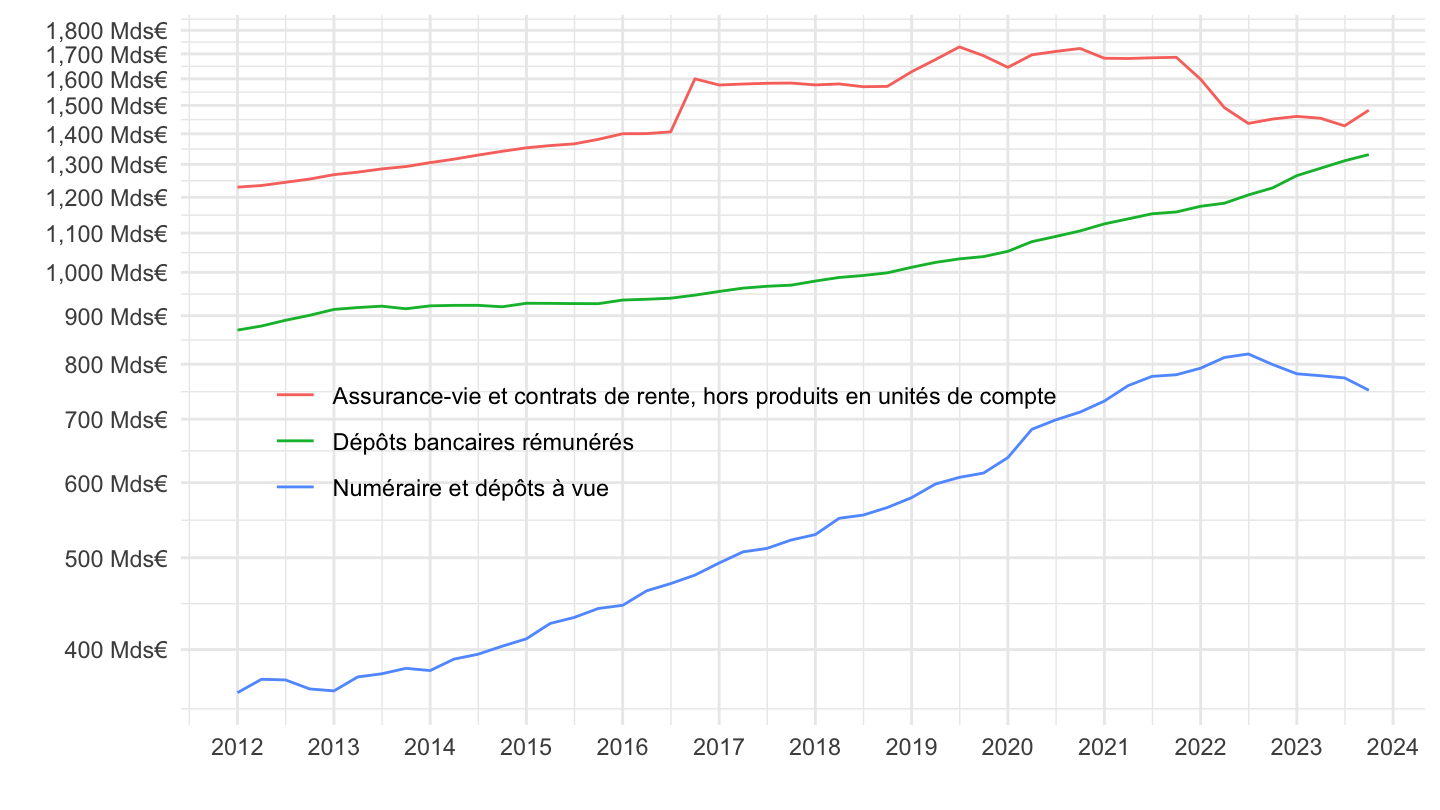

2019-

Code

CFT %>%
  left_join(CFT_var, by = "variable") %>%
  left_join(INSTR_ASSET, by = "INSTR_ASSET") %>%
  filter(REF_AREA %in% c("FR"),
         INSTR_ASSET %in% c("F2A", "F29Z", "F62B"),
         STO == "LE") %>%
  select(date, value, Instr_asset) %>%
  na.omit %>%
  filter(date >= as.Date("2022-01-01")) %>%
  ggplot + geom_line(aes(x = date, y = value, color = Instr_asset)) + 
  xlab("") + ylab("") + theme_minimal() +
  
  scale_x_date(breaks = "3 months",
               labels = date_format("%b %Y")) +
  scale_y_log10(breaks = seq(100, 4000, 100),
                labels = dollar_format(accuracy = 1, pre = "", su = " Mds€")) +
  theme(legend.position = c(0.4, 0.4),
        legend.title = element_blank(),
        legend.direction = "vertical") +
  geom_label(data = . %>% filter(date == as.Date("2023-12-31")),
             aes(x = date, y = value, color = Instr_asset, label = round(value)))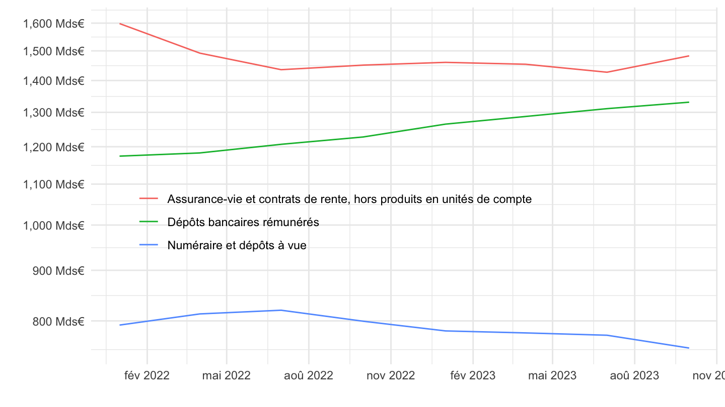

Flux - 4 trimestres

Code

CFT %>%
  left_join(CFT_var, by = "variable") %>%
  left_join(INSTR_ASSET, by = "INSTR_ASSET") %>%
  filter(REF_AREA %in% c("FR"),
         INSTR_ASSET %in% c("F2A", "F29Z", "F62B", "F29R"),
         STO == "F",
         TRANSFORMATION == "C4") %>%
  #filter(date >= as.Date("2016-01-01")) %>%
  select(date, value, Instr_asset) %>%
  na.omit %>%
  ggplot + geom_line(aes(x = date, y = value, color = Instr_asset)) + 
  xlab("") + ylab("") + theme_minimal() +
  
  scale_x_date(breaks = "1 year",
               labels = date_format("%Y")) +
  scale_y_continuous(breaks = seq(-2000, 4000, 10),
                labels = dollar_format(accuracy = 1, pre = "", su = " Mds€")) +
  theme(legend.position = c(0.4, 0.8),
        legend.title = element_blank(),
        legend.direction = "vertical")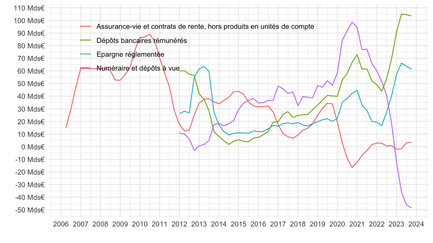

Flux

All

Code

CFT %>%
  left_join(CFT_var, by = "variable") %>%
  left_join(INSTR_ASSET, by = "INSTR_ASSET") %>%
  filter(REF_AREA %in% c("FR"),
         INSTR_ASSET %in% c("F2A", "F29Z", "F62B", "F29R"),
         STO == "F",
         TRANSFORMATION == "N",
         FREQ == "Q") %>%
  filter(date >= as.Date("2010-01-01")) %>%
  ggplot + geom_line(aes(x = date, y = value, color = Instr_asset)) + 
  xlab("") + ylab("") + theme_minimal() +
  
  scale_x_date(breaks = "1 year",
               labels = date_format("%Y")) +
  scale_y_continuous(breaks = seq(-1000, 4000, 10),
                labels = dollar_format(accuracy = 1, pre = "", su = " Mds€")) +
  theme(legend.position = c(0.4, 0.8),
        legend.title = element_blank(),
        legend.direction = "vertical")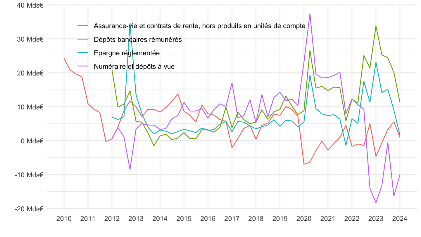

2016

Code

CFT %>%
  left_join(CFT_var, by = "variable") %>%
  left_join(INSTR_ASSET, by = "INSTR_ASSET") %>%
  filter(REF_AREA %in% c("FR"),
         INSTR_ASSET %in% c("F2A", "F29Z", "F62B", "F29R"),
         STO == "F",
         TRANSFORMATION == "N",
         FREQ == "Q") %>%
  filter(date >= as.Date("2016-01-01")) %>%
  ggplot + geom_line(aes(x = date, y = value, color = Instr_asset)) + 
  xlab("") + ylab("") + theme_minimal() +
  
  scale_x_date(breaks = "1 year",
               labels = date_format("%Y")) +
  scale_y_continuous(breaks = seq(-1000, 4000, 10),
                labels = dollar_format(accuracy = 1, pre = "", su = " Mds€")) +
  theme(legend.position = c(0.4, 0.9),
        legend.title = element_blank(),
        legend.direction = "vertical") +
  geom_hline(yintercept = 0, linetype = "dashed")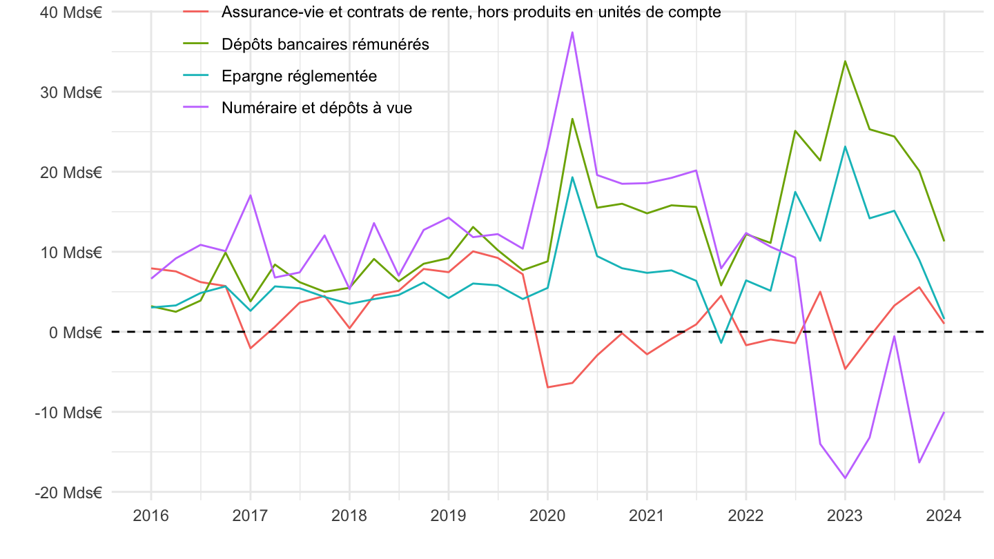

Actions côtées / non côtées, AV en unités de compte

Stocks

Code

CFT %>%
  left_join(CFT_var, by = "variable") %>%
  left_join(INSTR_ASSET, by = "INSTR_ASSET") %>%
  filter(REF_AREA %in% c("FR"),
         INSTR_ASSET %in% c( "F511", "F51M", "F51"),
         STO == "LE") %>%
  na.omit %>%
  ggplot + geom_line(aes(x = date, y = value, color = Instr_asset)) + 
  xlab("") + ylab("") + theme_minimal() +
  
  scale_x_date(breaks = "1 year",
               labels = date_format("%Y")) +
  scale_y_log10(breaks = seq(100, 4000, 100),
                labels = dollar_format(accuracy = 1, pre = "", su = " Mds€")) +
  theme(legend.position = c(0.4, 0.6),
        legend.title = element_blank(),
        legend.direction = "vertical") +
  geom_label(data = . %>% filter(date == as.Date("2023-12-31")),
             aes(x = date, y = value, color = Instr_asset, label = round(value)))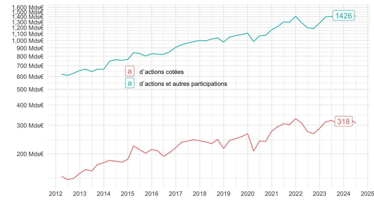

Actions côtées / non côtées, AV en unités de compte

Stocks

Code

CFT %>%
  left_join(CFT_var, by = "variable") %>%
  left_join(INSTR_ASSET, by = "INSTR_ASSET") %>%
  filter(REF_AREA %in% c("FR"),
         INSTR_ASSET %in% c( "F511", "F51M", "F62A"),
         STO == "LE") %>%
  na.omit %>%
  ggplot + geom_line(aes(x = date, y = value, color = Instr_asset)) + 
  xlab("") + ylab("") + theme_minimal() +
  
  scale_x_date(breaks = "1 year",
               labels = date_format("%Y")) +
  scale_y_log10(breaks = seq(100, 4000, 100),
                labels = dollar_format(accuracy = 1, pre = "", su = " Mds€")) +
  theme(legend.position = c(0.4, 0.6),
        legend.title = element_blank(),
        legend.direction = "vertical") +
  geom_label(data = . %>% filter(date == as.Date("2023-12-31")),
             aes(x = date, y = value, color = Instr_asset, label = round(value)))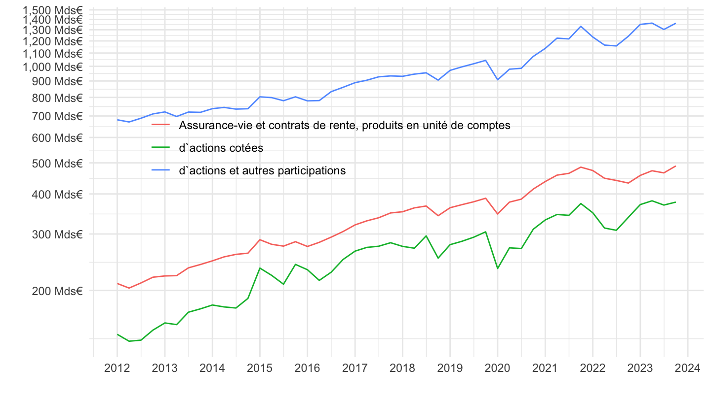

Flux

Code

CFT %>%
  left_join(CFT_var, by = "variable") %>%
  left_join(INSTR_ASSET, by = "INSTR_ASSET") %>%
  filter(REF_AREA %in% c("FR"),
         INSTR_ASSET %in% c( "F511", "F51M", "F62A"),
         STO == "F",
         TRANSFORMATION == "N",
         FREQ == "Q") %>%
  filter(date >= as.Date("2016-01-01")) %>%
  ggplot + geom_line(aes(x = date, y = value, color = Instr_asset)) + 
  xlab("") + ylab("") + theme_minimal() +
  
  scale_x_date(breaks = "1 year",
               labels = date_format("%Y")) +
  scale_y_continuous(breaks = seq(-2000, 4000, 5),
                labels = dollar_format(accuracy = 1, pre = "", su = " Mds€")) +
  theme(legend.position = c(0.4, 0.4),
        legend.title = element_blank(),
        legend.direction = "vertical")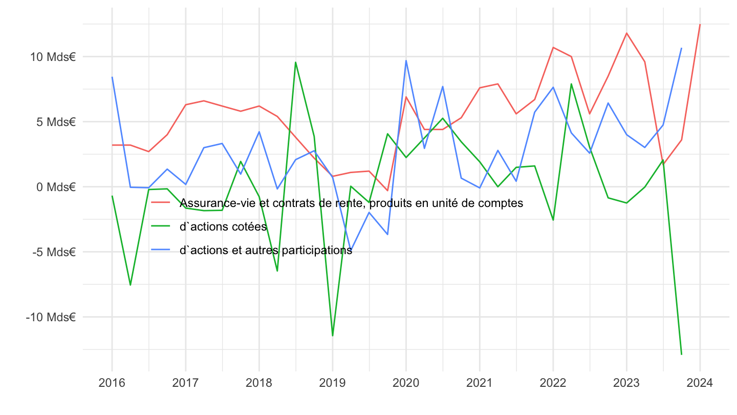

Numéraires et dépôts à vue

Code

CFT %>%
  left_join(CFT_var, by = "variable") %>%
  left_join(INSTR_ASSET, by = "INSTR_ASSET") %>%
  filter(REF_AREA %in% c("FR"),
         INSTR_ASSET %in% c("F2A", "F29Z"),
         STO == "LE") %>%
  na.omit %>%
  ggplot + geom_line(aes(x = date, y = value, color = Instr_asset)) + 
  xlab("") + ylab("") + theme_minimal() +
  
  scale_x_date(breaks = "1 year",
               labels = date_format("%Y")) +
  scale_y_log10(breaks = seq(100, 4000, 100),
                labels = dollar_format(accuracy = 1, pre = "", su = " Mds€")) +
  theme(legend.position = c(0.75, 0.1),
        legend.title = element_blank(),
        legend.direction = "vertical") +
  geom_label(data = . %>% filter(date == as.Date("2023-12-31")),
             aes(x = date, y = value, color = Instr_asset, label = round(value)))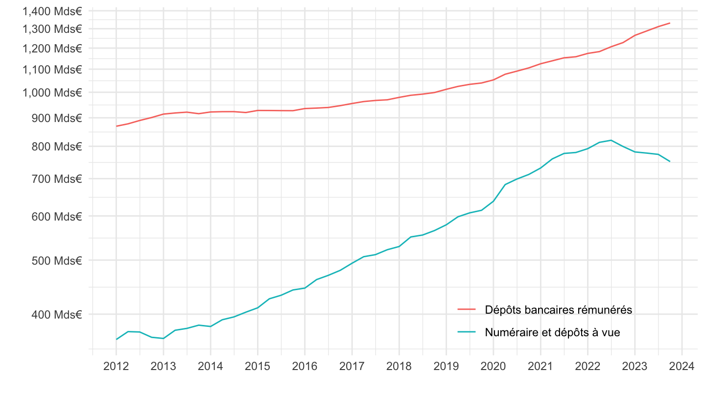

Assurance Vie

Toutes

2007-

Code

CFT %>%
  left_join(CFT_var, by = "variable") %>%
  filter(variable %in% c("CFT.Q.S.FR.W0.S1M.S1.N.A.F.F62B._Z._Z.XDC._T.S.V.N._T",
                         "CFT.Q.S.FR.W0.S1M.S1.N.A.F.F62A._Z._Z.XDC._T.S.V.N._T",
                         "CFT.Q.S.FR.W0.S1M.S1.N.A.F.F29R.T._Z.XDC._T.S.V.N._T",
                         "CFT.Q.S.FR.W0.S1M.S1.N.A.F.F2A.T._Z.XDC._T.S.V.N._T")) %>%
  na.omit %>%
  ggplot + geom_line(aes(x = date, y = value, color = Variable)) + 
  xlab("") + ylab("") + theme_minimal() +
  
  scale_x_date(breaks = "1 year",
               labels = date_format("%Y")) +
  scale_y_continuous(breaks = seq(-200, 1000, 5),
                     limits = c(-25 ,40),
                     labels = dollar_format(acc = 1, prefix = "", su = "Mds€")) +
  theme(legend.position = c(0.45, 0.17),
        legend.title = element_blank(),
        legend.direction = "vertical")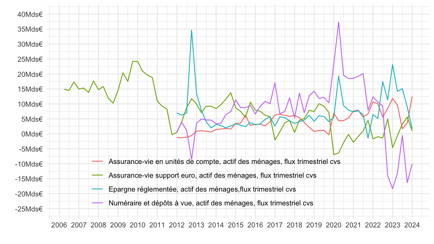

2015-

Code

CFT %>%
  left_join(CFT_var, by = "variable") %>%
  filter(variable %in% c("CFT.Q.S.FR.W0.S1M.S1.N.A.F.F62B._Z._Z.XDC._T.S.V.N._T",
                         "CFT.Q.S.FR.W0.S1M.S1.N.A.F.F29Z.T._Z.XDC._T.S.V.N._T",
                         "CFT.Q.S.FR.W0.S1M.S1.N.A.F.F29R.T._Z.XDC._T.S.V.N._T",
                         "CFT.Q.S.FR.W0.S1M.S1.N.A.F.F2A.T._Z.XDC._T.S.V.N._T")) %>%
  filter(date >= as.Date("2015-01-01")) %>%
  ggplot + geom_line(aes(x = date, y = value, color = Variable)) + 
  xlab("") + ylab("") + theme_minimal() +
  
  scale_x_date(breaks = "1 year",
               labels = date_format("%Y")) +
  scale_y_continuous(breaks = seq(-200, 1000, 5),
                     limits = c(-5 ,40),
                     labels = dollar_format(acc = 1, prefix = "", su = "Mds€")) +
  theme(legend.position = c(0.45, 0.8),
        legend.title = element_blank(),
        legend.direction = "vertical")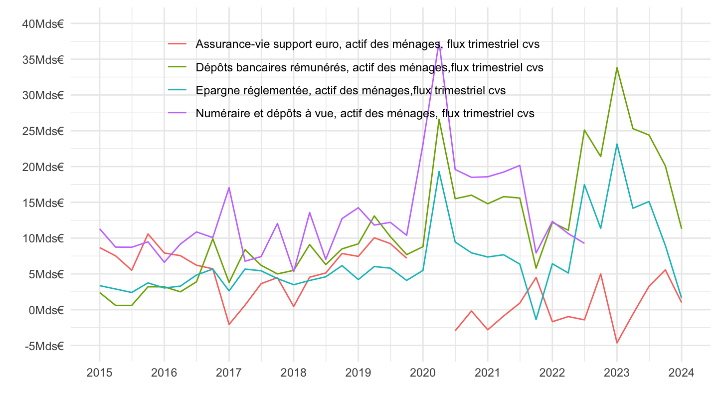

Taux d’épargne des ménages

Le taux d’épargne des ménages est le rapport entre l’épargne brute des ménages (B8G) et le revenu disponible brut ajusté des variations de droits à pension. Le revenu disponible brut (B6G) correspond aux revenus que perçoivent les ménages (revenus d’activité et revenus fonciers) après opérations de redistribution (ajout des prestations sociales en espèces reçues, soustraction des cotisations et impôts).

Quant au taux d’épargne financière, il s’agit de la part du revenu disponible brut investie dans des actifs financiers.

le taux d’épargne s’obtient en rapportant l’épargne brute au revenu disponible brut ajusté de la variation des droits des ménages sur les fonds de pension, préalablement corrigés des variations saisonnières
le taux d’épargne financière est estimé en soustrayant la formation brute de capital fixe à l’épargne brute, ensuite rapportée au revenu disponible brut ajusté de la variation des droits des ménages sur les fonds de pension, puis en corrigeant des variations saisonnières.

France

Annual

Code

CFT %>%
  left_join(CFT_var, by = "variable") %>%
  filter(variable %in% c("CFT.A.N.FR.W0.S1M.S1.N.B.B8G._Z._Z._Z.XDC_R_B6G_S1M._T.S.V.N._T",
                         "CFT.A.N.FR.W0.S1M.S1.N.B.B9Z._Z._Z._Z.XDC_R_B6G_S1M._T.S.V.N._T")) %>%
  na.omit %>%
  ggplot + geom_line(aes(x = date, y = value/100, color = Variable)) + 
  xlab("") + ylab("") + theme_minimal() +
  
  scale_x_date(breaks = "1 year",
               labels = date_format("%Y")) +
  scale_y_continuous(breaks = 0.01*seq(-10, 100, 1),
                labels = percent_format(accuracy = 1)) +
  theme(legend.position = c(0.4, 0.9),
        legend.title = element_blank(),
        legend.direction = "vertical")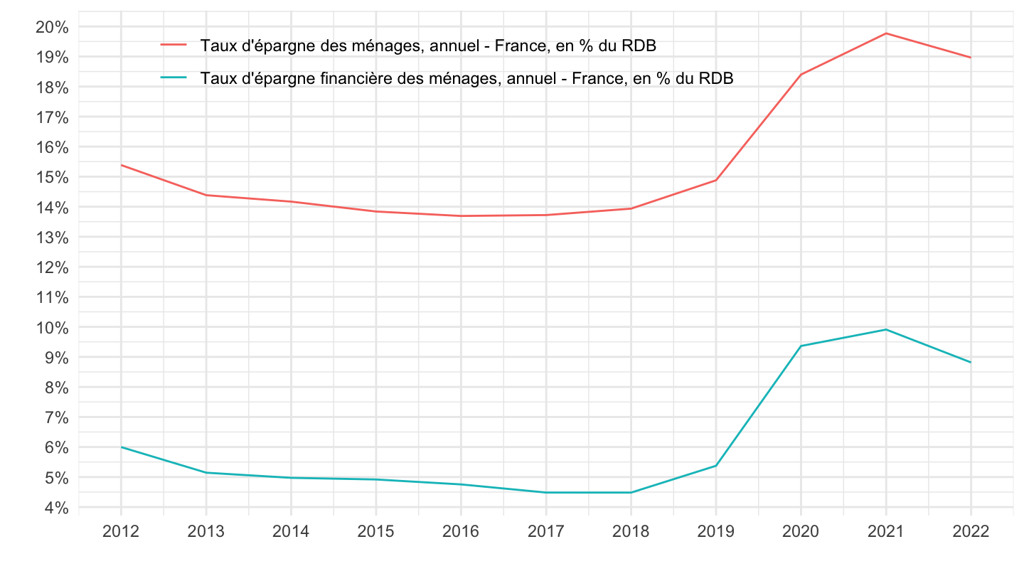

Quarterly

All

Code

CFT %>%
  left_join(CFT_var, by = "variable") %>%
  filter(variable %in% c("CFT.Q.N.FR.W0.S1M.S1.N.B.B8G._Z._Z._Z.XDC_R_B6G_S1M._T.S.V.C4._T",
                         "CFT.Q.N.FR.W0.S1M.S1.N.B.B9Z._Z._Z._Z.XDC_R_B6G_S1M._T.S.V.C4._T")) %>%
  na.omit %>%
  ggplot + geom_line(aes(x = date, y = value/100, color = Variable)) + 
  xlab("") + ylab("") + theme_minimal() +
  scale_x_date(breaks = "2 years",
               labels = date_format("%Y")) +
  scale_y_continuous(breaks = 0.01*seq(-10, 100, 1),
                labels = percent_format(accuracy = 1)) +
  theme(legend.position = c(0.42, 0.9),
        legend.title = element_blank(),
        legend.direction = "vertical")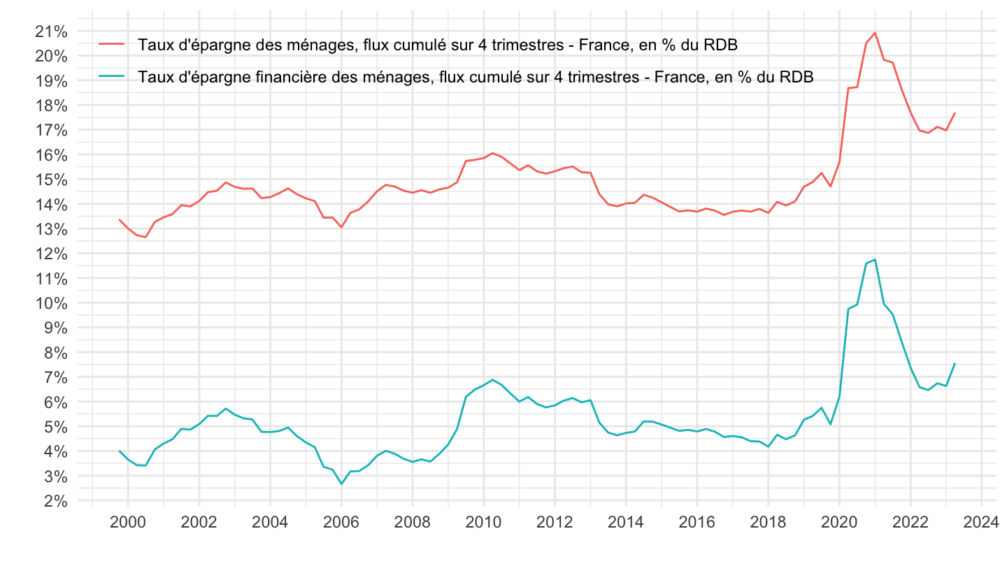

2010-

Code

CFT %>%
  left_join(CFT_var, by = "variable") %>%
  filter(variable %in% c("CFT.Q.N.FR.W0.S1M.S1.N.B.B8G._Z._Z._Z.XDC_R_B6G_S1M._T.S.V.C4._T",
                         "CFT.Q.N.FR.W0.S1M.S1.N.B.B9Z._Z._Z._Z.XDC_R_B6G_S1M._T.S.V.C4._T")) %>%
  na.omit %>%
  filter(date >= as.Date("2010-01-01")) %>%
  ggplot + geom_line(aes(x = date, y = value/100, color = Variable)) + 
  xlab("") + ylab("") + theme_minimal() +
  scale_x_date(breaks = "2 years",
               labels = date_format("%Y")) +
  scale_y_continuous(breaks = 0.01*seq(-10, 100, 1),
                labels = percent_format(accuracy = 1)) +
  theme(legend.position = c(0.45, 0.9),
        legend.title = element_blank(),
        legend.direction = "vertical")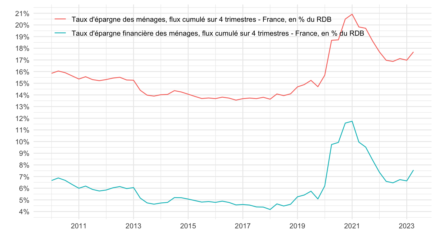

France, Spain, Italy

Table

Code

load_data("bdf/REF_AREA.RData")
CFT %>%
  left_join(CFT_var, by = "variable") %>%
  left_join(REF_AREA, by = "REF_AREA") %>%
  filter(FREQ == "Q",
         UNIT_MEASURE == "XDC_R_B6G_S1M",
         REF_SECTOR == "S1M",
         date == as.Date("2020-01-01")) %>%
  select(Variable, Ref_area, value) %>%
  arrange(Ref_area) %>%
  print_table_conditional

Variable	Ref_area	value
NA	NA	NA
:--------:	:--------:	:-----:

Taux d’épargne financière

France, Italy, Germany

Code

CFT %>%
  left_join(CFT_var, by = "variable") %>%
  left_join(REF_AREA, by = "REF_AREA") %>%
  filter(FREQ == "Q",
         REF_AREA %in% c("FR", "IT", "DE"),
         UNIT_MEASURE == "XDC_R_B6G_S1M",
         STO == "B9Z",
         REF_SECTOR == "S1M") %>%
  mutate(value = value/100) %>%
  na.omit %>%
  ggplot + geom_line(aes(x = date, y = value, color = Ref_area)) + 
  xlab("") + ylab("") + theme_minimal() +
  scale_color_manual(values = c("#002395", "#000000", "#009246")) +
  scale_x_date(breaks = "2 years",
               labels = date_format("%Y")) +
  add_3flags +
  scale_y_continuous(breaks = 0.01*seq(-10, 100, 1),
                labels = percent_format(accuracy = 1)) +
  theme(legend.position = "none")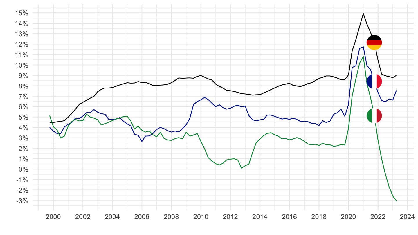

France, Italy, Germany, Spain, United States

All

Code

CFT %>%
  left_join(CFT_var, by = "variable") %>%
  left_join(REF_AREA, by = "REF_AREA") %>%
  filter(FREQ == "Q",
         UNIT_MEASURE == "XDC_R_B6G_S1M",
         STO == "B9Z",
         REF_SECTOR == "S1M") %>%
  left_join(colors, by = c("Ref_area" = "country")) %>%
  mutate(value = value/100) %>%
  na.omit %>%
  ggplot + geom_line(aes(x = date, y = value, color = color)) + 
  xlab("") + ylab("") + theme_minimal() + scale_color_identity() + add_6flags +
  scale_x_date(breaks = "2 years",
               labels = date_format("%Y")) +
  scale_y_continuous(breaks = 0.01*seq(-10, 100, 1),
                labels = percent_format(accuracy = 1))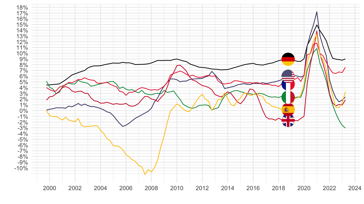

2007-

Code

CFT %>%
  left_join(CFT_var, by = "variable") %>%
  left_join(REF_AREA, by = "REF_AREA") %>%
  filter(FREQ == "Q",
         UNIT_MEASURE == "XDC_R_B6G_S1M",
         STO == "B9Z",
         REF_SECTOR == "S1M") %>%
  left_join(colors, by = c("Ref_area" = "country")) %>%
  mutate(value = value/100) %>%
  filter(date >= as.Date("2007-01-01")) %>%
  na.omit %>%
  ggplot + geom_line(aes(x = date, y = value, color = color)) + 
  xlab("") + ylab("") + theme_minimal() + scale_color_identity() + add_6flags +
  scale_x_date(breaks = "1 year",
               labels = date_format("%Y")) +
  scale_y_continuous(breaks = 0.01*seq(-10, 100, 1),
                labels = percent_format(accuracy = 1))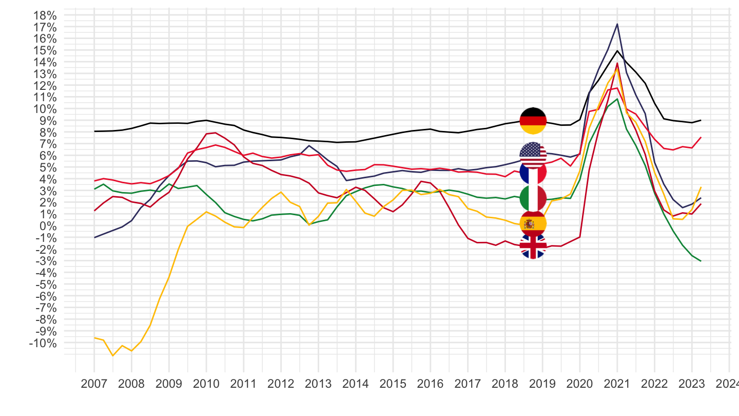

2015-

Code

CFT %>%
  left_join(CFT_var, by = "variable") %>%
  left_join(REF_AREA, by = "REF_AREA") %>%
  filter(FREQ == "Q",
         UNIT_MEASURE == "XDC_R_B6G_S1M",
         STO == "B9Z",
         REF_SECTOR == "S1M") %>%
  left_join(colors, by = c("Ref_area" = "country")) %>%
  mutate(value = value/100) %>%
  filter(date >= as.Date("2015-01-01")) %>%
  na.omit %>%
  ggplot + geom_line(aes(x = date, y = value, color = color)) + 
  xlab("") + ylab("Taux d'épargne financière (%)") + theme_minimal() + scale_color_identity() + add_6flags +
  scale_x_date(breaks = "1 year",
               labels = date_format("%Y")) +
  scale_y_continuous(breaks = 0.01*seq(-10, 100, 1),
                labels = percent_format(accuracy = 1))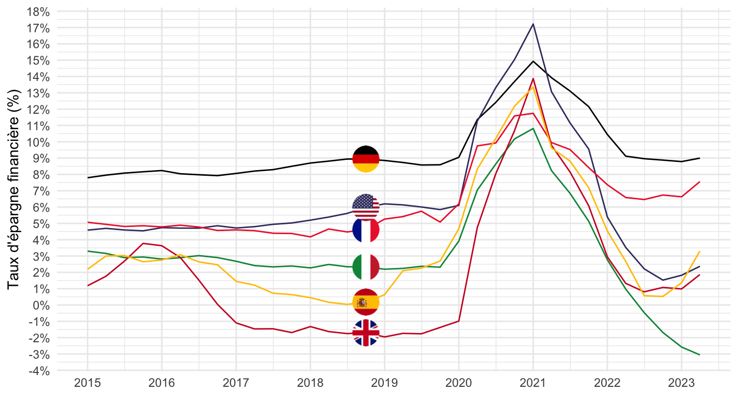

Taux d’épargne

France, Italy, Germany

Code

CFT %>%
  left_join(CFT_var, by = "variable") %>%
  left_join(REF_AREA, by = "REF_AREA") %>%
  filter(FREQ == "Q",
         REF_AREA %in% c("FR", "IT", "DE"),
         UNIT_MEASURE == "XDC_R_B6G_S1M",
         STO == "B8G",
         REF_SECTOR == "S1M") %>%
  left_join(colors, by = c("Ref_area" = "country")) %>%
  mutate(value = value/100) %>%
  na.omit %>%
  ggplot + geom_line(aes(x = date, y = value, color = color)) + 
  xlab("") + ylab("") + theme_minimal() + scale_color_identity() + add_3flags +
  scale_x_date(breaks = "2 years",
               labels = date_format("%Y")) +
  scale_y_continuous(breaks = 0.01*seq(-10, 100, 1),
                labels = percent_format(accuracy = 1))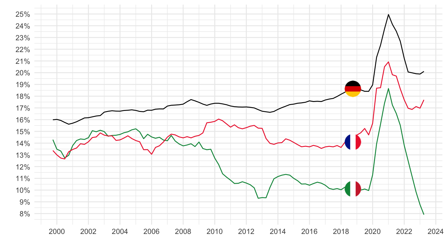

France, Italy, Germany, Spain, United States

Code

CFT %>%
  left_join(CFT_var, by = "variable") %>%
  left_join(REF_AREA, by = "REF_AREA") %>%
  filter(FREQ == "Q",
         UNIT_MEASURE == "XDC_R_B6G_S1M",
         STO == "B8G",
         REF_SECTOR == "S1M") %>%
  left_join(colors, by = c("Ref_area" = "country")) %>%
  mutate(value = value/100) %>%
  na.omit %>%
  ggplot + geom_line(aes(x = date, y = value, color = color)) + 
  xlab("") + ylab("") + theme_minimal() + scale_color_identity() + add_6flags +
  scale_x_date(breaks = "2 years",
               labels = date_format("%Y")) +
  scale_y_continuous(breaks = 0.01*seq(-10, 100, 1),
                labels = percent_format(accuracy = 1))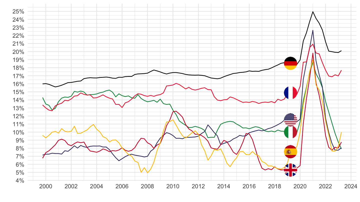

Dette

Dette des ménages

All

Code

CFT %>%
  left_join(CFT_var, by = "variable") %>%
  left_join(REF_AREA, by = "REF_AREA") %>%
  filter(INSTR_ASSET == "DETT",
         UNIT_MEASURE == "XDC_R_B1GQ_CY",
         REF_SECTOR == "S1M") %>%
  mutate(Ref_area = ifelse(REF_AREA == "I8", "Europe", Ref_area)) %>%
  mutate(Ref_area = ifelse(REF_AREA == "UK", "United Kingdom", Ref_area)) %>%
  left_join(colors, by = c("Ref_area" = "country")) %>%
  mutate(value = value/100) %>%
  arrange(date) %>%
  select(REF_AREA,everything()) %>%
  ggplot + geom_line(aes(x = date, y = value, color = color)) + 
  xlab("") + ylab("") + theme_minimal() + scale_color_identity() + add_7flags +
  scale_x_date(breaks = "2 years",
               labels = date_format("%Y")) +
  scale_y_continuous(breaks = 0.01*seq(-10, 200, 10),
                labels = percent_format(accuracy = 1))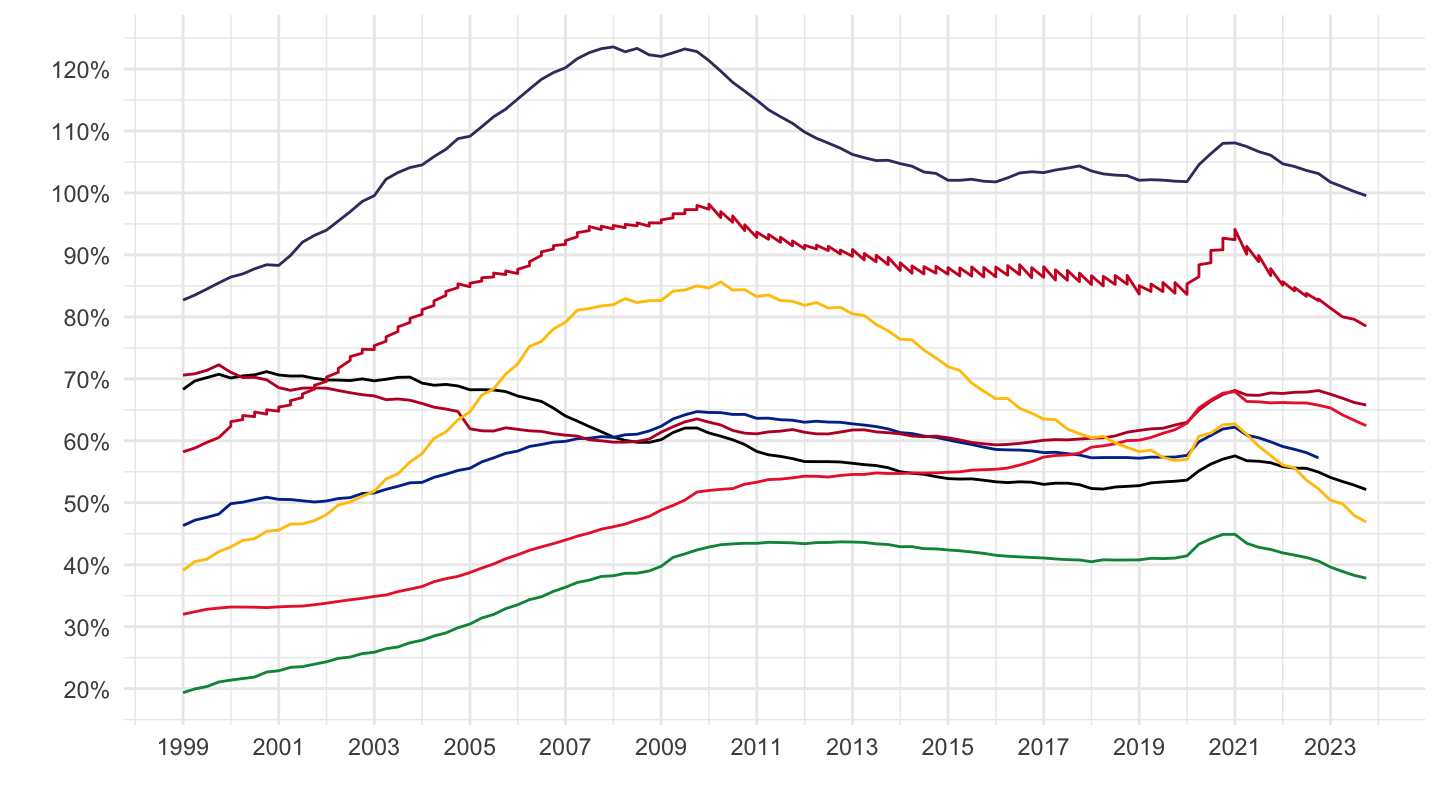

France, Italy, Germany, Spain, Japan, EU

Code

CFT %>%
  left_join(CFT_var, by = "variable") %>%
  left_join(REF_AREA, by = "REF_AREA") %>%
  filter(REF_AREA %in% c("FR", "IT", "DE", "ES", "JP", "I8"),
         INSTR_ASSET == "DETT",
         UNIT_MEASURE == "XDC_R_B1GQ_CY",
         REF_SECTOR == "S1M") %>%
  mutate(Ref_area = ifelse(REF_AREA == "I8", "Europe", Ref_area)) %>%
  left_join(colors, by = c("Ref_area" = "country")) %>%
  mutate(value = value/100) %>%
  ggplot + geom_line(aes(x = date, y = value, color = color)) + 
  xlab("") + ylab("") + theme_minimal() + scale_color_identity() + add_6flags +
  scale_x_date(breaks = "2 years",
               labels = date_format("%Y")) +
  scale_y_continuous(breaks = 0.01*seq(-10, 100, 5),
                labels = percent_format(accuracy = 1))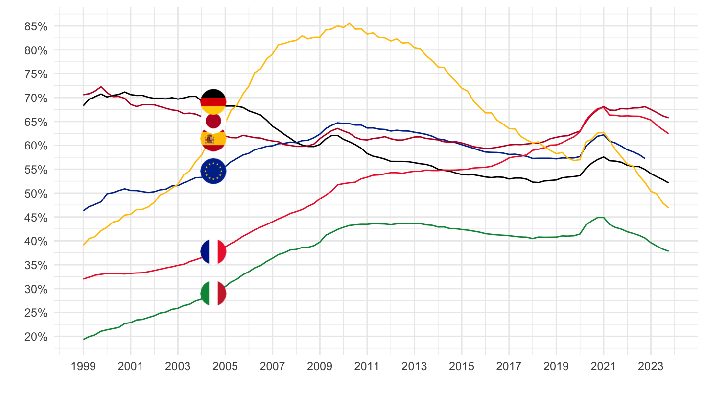

France, Italy, Germany

All

Code

CFT %>%
  left_join(CFT_var, by = "variable") %>%
  left_join(REF_AREA, by = "REF_AREA") %>%
  filter(REF_AREA %in% c("FR", "IT", "DE"),
         INSTR_ASSET == "DETT",
         UNIT_MEASURE == "XDC_R_B1GQ_CY",
         REF_SECTOR == "S1M") %>%
  mutate(Ref_area = ifelse(REF_AREA == "I8", "Europe", Ref_area)) %>%
  left_join(colors, by = c("Ref_area" = "country")) %>%
  mutate(value = value/100) %>%
  ggplot + geom_line(aes(x = date, y = value, color = color)) + 
  xlab("") + ylab("") + theme_minimal() + scale_color_identity() + add_3flags +
  scale_x_date(breaks = "2 years",
               labels = date_format("%Y")) +
  scale_y_continuous(breaks = 0.01*seq(-10, 100, 5),
                labels = percent_format(accuracy = 1))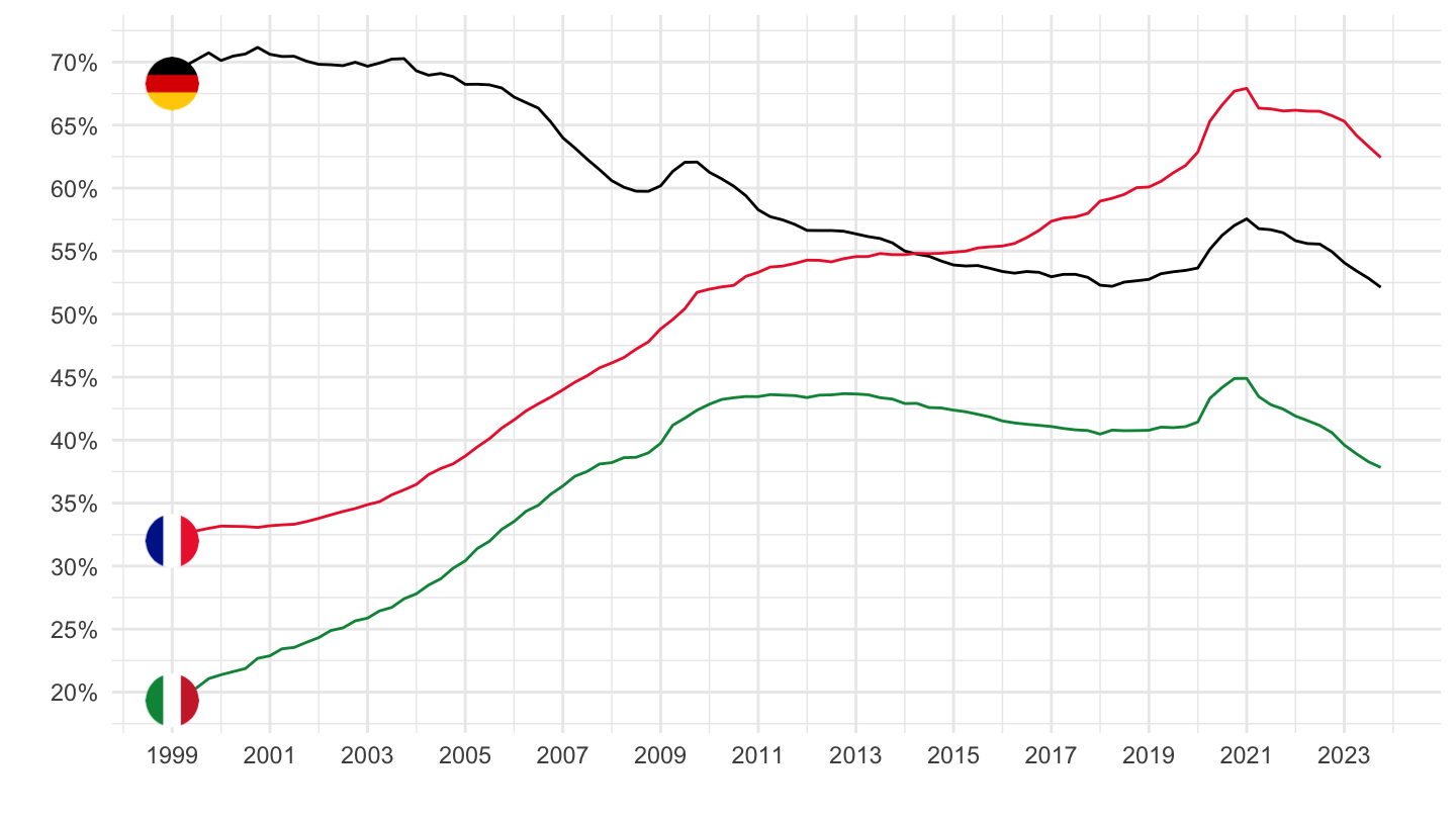

2013-

Code

CFT %>%
  left_join(CFT_var, by = "variable") %>%
  left_join(REF_AREA, by = "REF_AREA") %>%
  filter(REF_AREA %in% c("FR", "IT", "DE"),
         INSTR_ASSET == "DETT",
         UNIT_MEASURE == "XDC_R_B1GQ_CY",
         REF_SECTOR == "S1M") %>%
  mutate(Ref_area = ifelse(REF_AREA == "I8", "Europe", Ref_area)) %>%
  left_join(colors, by = c("Ref_area" = "country")) %>%
  mutate(value = value/100) %>%
  filter(date >=as.Date("2013-01-01")) %>%
  ggplot + geom_line(aes(x = date, y = value, color = color)) + 
  xlab("") + ylab("") + theme_minimal() + scale_color_identity() + add_3flags +
  scale_x_date(breaks = "1 year",
               labels = date_format("%Y")) +
  scale_y_continuous(breaks = 0.01*seq(-10, 100, 2),
                labels = percent_format(accuracy = 1))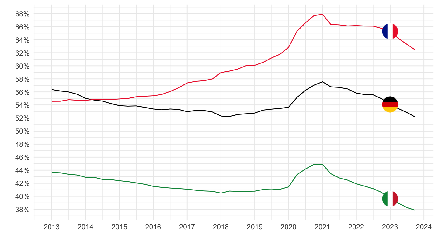

Non-financial corporations

France, Italy, Germany

Code

CFT %>%
  left_join(CFT_var, by = "variable") %>%
  left_join(REF_AREA, by = "REF_AREA") %>%
  filter(REF_AREA %in% c("FR", "IT", "DE", "I8"),
         INSTR_ASSET == "DETT",
         UNIT_MEASURE == "XDC_R_B1GQ_CY",
         REF_SECTOR == "S11") %>%
  mutate(Ref_area = ifelse(REF_AREA == "I8", "Europe", Ref_area)) %>%
  left_join(colors, by = c("Ref_area" = "country")) %>%
  mutate(value = value/100) %>%
  ggplot + geom_line(aes(x = date, y = value, color = color)) + 
  xlab("") + ylab("") + theme_minimal() + scale_color_identity() + add_4flags +
  scale_x_date(breaks = "2 years",
               labels = date_format("%Y")) +
  scale_y_continuous(breaks = 0.01*seq(-10, 100, 5),
                labels = dollar_format(accuracy = .01, pre = "", su = " année"))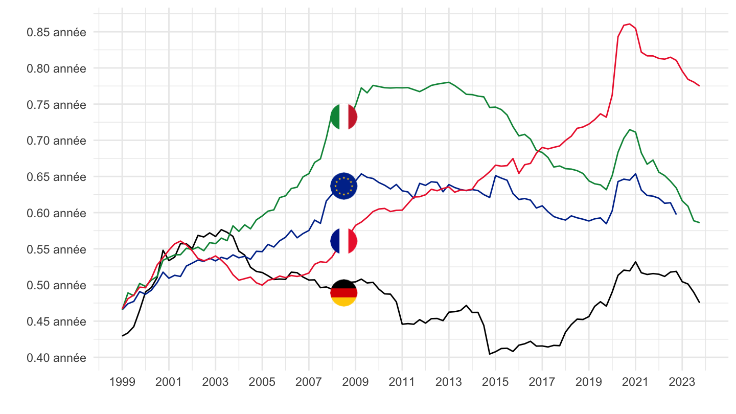

Taux d’endettement

France

Années de PIB

Code

CFT %>%
  left_join(CFT_var, by = "variable") %>%
  filter(variable %in% c("CFT.Q.S.FR.W0.S1M.S1.N.L.LE.DETT.T._Z.XDC_R_B1GQ_CY._T.S.V.N._T",
                         "CFT.Q.S.FR.W0.S11.S1.C.L.LE.DETT.T._Z.XDC_R_B1GQ_CY._T.S.V.N._T",
                         "CFT.Q.N.FR.W0.S13.S1.C.L.LE.GD.T._Z.XDC_R_B1GQ_CY._T.F.V.N._T")) %>%
  mutate(Variable = gsub(", en % du PIB", "", Variable),
         Variable = gsub(" en % du PIB", "", Variable)) %>%
  ggplot + geom_line(aes(x = date, y = value/100, color = Variable)) + 
  xlab("") + ylab("Dette/PIB (en années de PIB)") + theme_minimal() +
  
  scale_x_date(breaks = "2 years",
               labels = date_format("%Y")) +
  scale_y_continuous(breaks = seq(0, 1.3, 0.1),
                     labels = dollar_format(su = " ans", p = "", acc = 0.1)) +
  theme(legend.position = c(0.3, 0.9),
        legend.title = element_blank(),
        legend.direction = "vertical")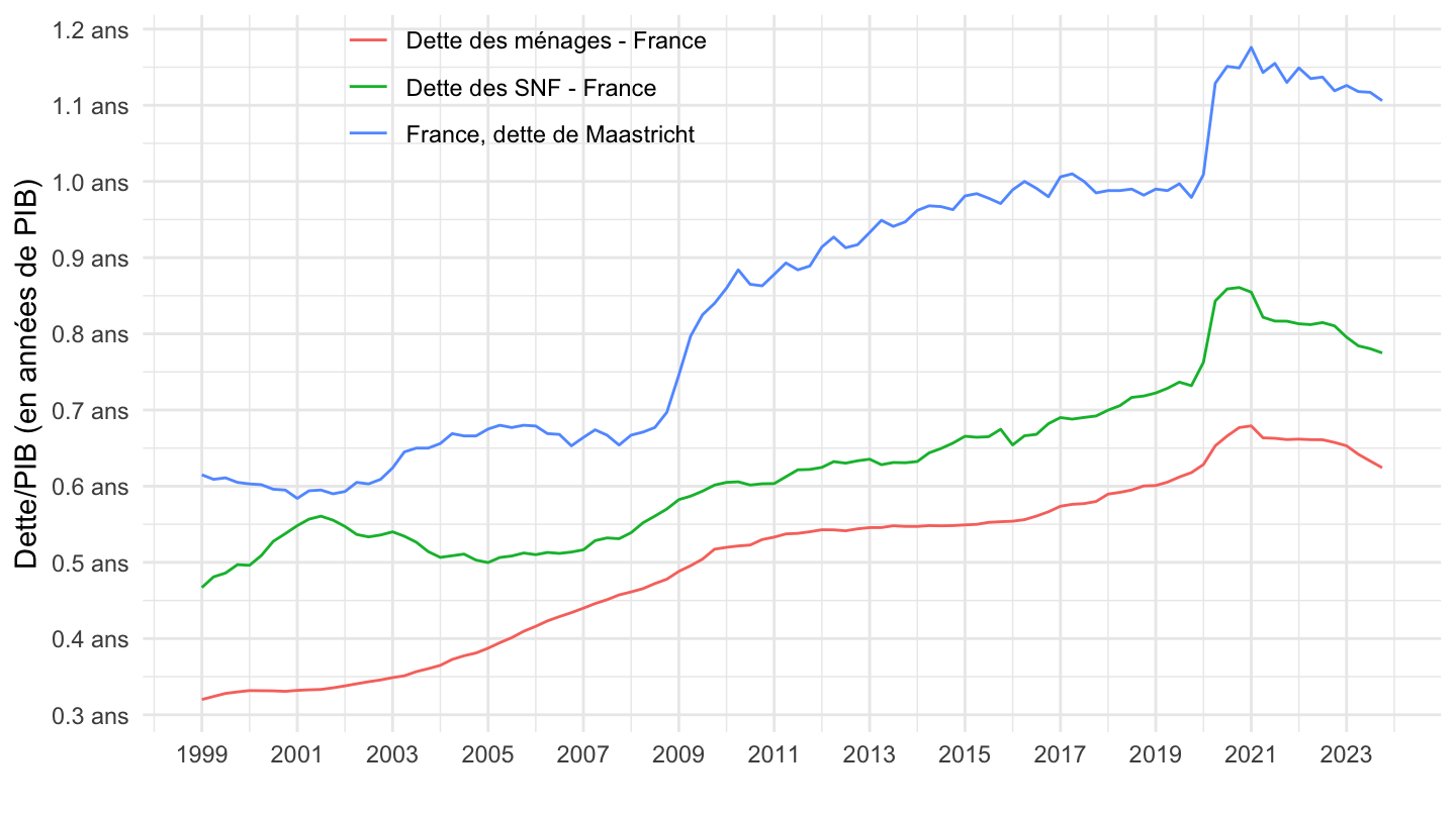

% du PIB

Code

CFT %>%
  left_join(CFT_var, by = "variable") %>%
  filter(variable %in% c("CFT.Q.S.FR.W0.S1M.S1.N.L.LE.DETT.T._Z.XDC_R_B1GQ_CY._T.S.V.N._T",
                         "CFT.Q.S.FR.W0.S11.S1.C.L.LE.DETT.T._Z.XDC_R_B1GQ_CY._T.S.V.N._T",
                         "CFT.Q.N.FR.W0.S13.S1.C.L.LE.GD.T._Z.XDC_R_B1GQ_CY._T.F.V.N._T")) %>%
  ggplot + geom_line(aes(x = date, y = value/100, color = Variable)) + 
  xlab("") + ylab("") + theme_minimal() +
  
  scale_x_date(breaks = "2 years",
               labels = date_format("%Y")) +
  scale_y_continuous(breaks = 0.01*seq(-10, 140, 5),
                labels = percent_format(accuracy = 1)) +
  theme(legend.position = c(0.3, 0.9),
        legend.title = element_blank(),
        legend.direction = "vertical")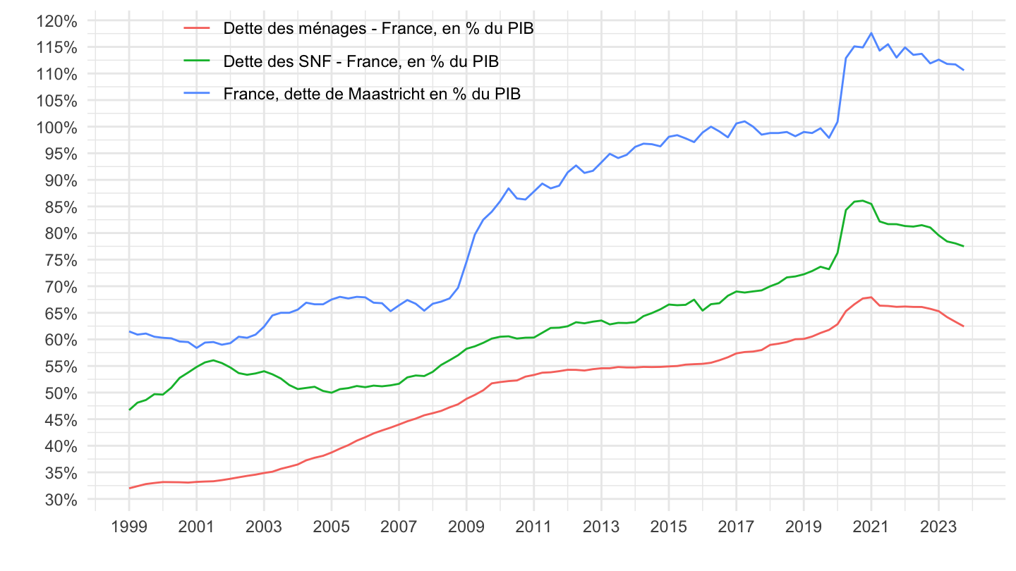

Allemagne

Code

CFT %>%
  left_join(CFT_var, by = "variable") %>%
  filter(variable %in% c("CFT.Q.N.DE.W0.S1M.S1.N.L.LE.DETT.T._Z.XDC_R_B1GQ_CY._T.S.V.N._T",
                         "CFT.Q.N.DE.W0.S11.S1.C.L.LE.DETT.T._Z.XDC_R_B1GQ_CY._T.S.V.N._T",
                         "CFT.Q.N.DE.W0.S13.S1.C.L.LE.GD.T._Z.XDC_R_B1GQ_CY._T.F.V.N._T")) %>%
  ggplot + geom_line(aes(x = date, y = value/100, color = Variable)) + 
  xlab("") + ylab("") + theme_minimal() +
  
  scale_x_date(breaks = "2 years",
               labels = date_format("%Y")) +
  scale_y_continuous(breaks = 0.01*seq(-10, 140, 5),
                labels = percent_format(accuracy = 1)) +
  theme(legend.position = c(0.3, 0.9),
        legend.title = element_blank(),
        legend.direction = "vertical")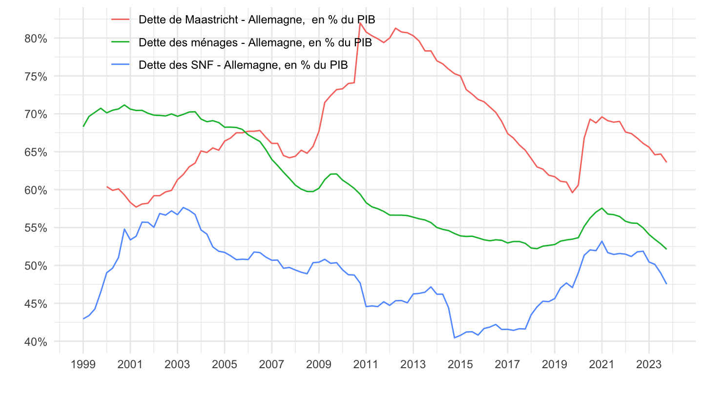

Italie

Code

CFT %>%
  left_join(CFT_var, by = "variable") %>%
  filter(variable %in% c("CFT.Q.N.IT.W0.S1M.S1.N.L.LE.DETT.T._Z.XDC_R_B1GQ_CY._T.S.V.N._T",
                         "CFT.Q.N.IT.W0.S11.S1.C.L.LE.DETT.T._Z.XDC_R_B1GQ_CY._T.S.V.N._T",
                         "CFT.Q.N.IT.W0.S13.S1.C.L.LE.GD.T._Z.XDC_R_B1GQ_CY._T.F.V.N._T")) %>%
  ggplot + geom_line(aes(x = date, y = value/100, color = Variable)) + 
  xlab("") + ylab("") + theme_minimal() +
  
  scale_x_date(breaks = "2 years",
               labels = date_format("%Y")) +
  scale_y_continuous(breaks = 0.01*seq(-10, 400, 10),
                labels = percent_format(accuracy = 1)) +
  theme(legend.position = c(0.3, 0.9),
        legend.title = element_blank(),
        legend.direction = "vertical")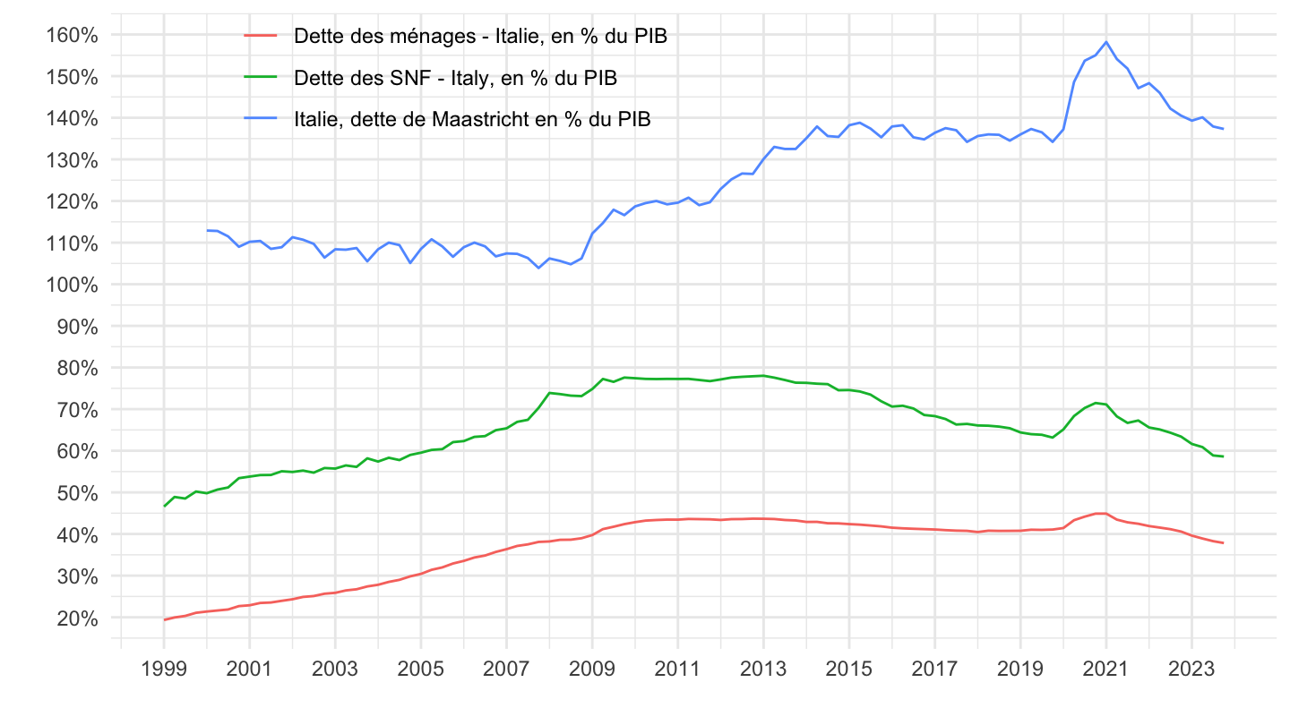

Espagne

Code

CFT %>%
  left_join(CFT_var, by = "variable") %>%
  filter(variable %in% c("CFT.Q.N.ES.W0.S1M.S1.N.L.LE.DETT.T._Z.XDC_R_B1GQ_CY._T.S.V.N._T",
                         "CFT.Q.N.ES.W0.S11.S1.C.L.LE.DETT.T._Z.XDC_R_B1GQ_CY._T.S.V.N._T",
                         "CFT.Q.N.ES.W0.S13.S1.C.L.LE.GD.T._Z.XDC_R_B1GQ_CY._T.F.V.N._T")) %>%
  ggplot + geom_line(aes(x = date, y = value/100, color = Variable)) + 
  xlab("") + ylab("") + theme_minimal() +
  
  scale_x_date(breaks = "2 years",
               labels = date_format("%Y")) +
  scale_y_continuous(breaks = 0.01*seq(-10, 400, 10),
                labels = percent_format(accuracy = 1)) +
  theme(legend.position = c(0.2, 0.9),
        legend.title = element_blank(),
        legend.direction = "vertical")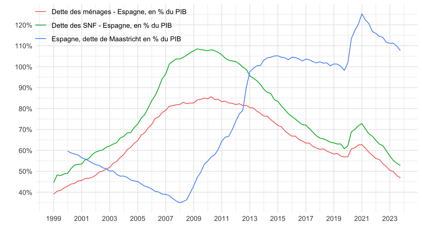

Zone Euro

Code

CFT %>%
  left_join(CFT_var, by = "variable") %>%
  filter(variable %in% c("CFT.Q.N.I8.W0.S1M.S1.N.L.LE.DETT.T._Z.XDC_R_B1GQ_CY._T.S.V.N._T",
                         "CFT.Q.N.I8.W0.S11.S1.C.L.LE.DETT.T._Z.XDC_R_B1GQ_CY._T.S.V.N._T",
                         "CFT.Q.N.I8.W0.S13.S1.C.L.LE.GD.T._Z.XDC_R_B1GQ_CY._T.F.V.N._T")) %>%
  ggplot + geom_line(aes(x = date, y = value/100, color = Variable)) + 
  xlab("") + ylab("") + theme_minimal() +
  
  scale_x_date(breaks = "2 years",
               labels = date_format("%Y")) +
  scale_y_continuous(breaks = 0.01*seq(-10, 140, 5),
                labels = percent_format(accuracy = 1)) +
  theme(legend.position = c(0.3, 0.9),
        legend.title = element_blank(),
        legend.direction = "vertical")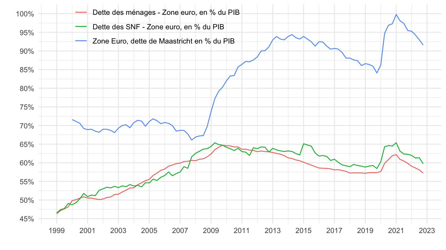

Informations supplémentaires

Données sur la macroéconomie en France

source	dataset	Title	.html	.rData
bdf	CFT	Comptes Financiers Trimestriels	2025-12-20	2025-03-09
insee	CNA-2014-CONSO-SI	Dépenses de consommation finale par secteur institutionnel	2025-12-23	2025-12-23
insee	CNA-2014-CSI	Comptes des secteurs institutionnels	2025-12-23	2025-12-23
insee	CNA-2014-FBCF-BRANCHE	Formation brute de capital fixe (FBCF) par branche	2025-12-23	2025-12-23
insee	CNA-2014-FBCF-SI	Formation brute de capital fixe (FBCF) par secteur institutionnel	2025-12-23	2025-12-23
insee	CNA-2014-RDB	Revenu et pouvoir d’achat des ménages	2025-12-23	2025-12-23
insee	CNA-2020-CONSO-MEN	Consommation des ménages	2025-12-23	2025-09-30
insee	CNA-2020-PIB	Produit intérieur brut (PIB) et ses composantes	2025-12-23	2025-05-28
insee	CNT-2014-CB	Comptes des branches	2025-12-23	2025-12-23
insee	CNT-2014-CSI	Comptes de secteurs institutionnels	2025-12-23	2025-12-23
insee	CNT-2014-OPERATIONS	Opérations sur biens et services	2025-12-23	2025-12-23
insee	CNT-2014-PIB-EQB-RF	Équilibre du produit intérieur brut	2025-12-23	2025-12-23
insee	CONSO-MENAGES-2020	Consommation des ménages en biens	2025-12-23	2025-12-23
insee	ICA-2015-IND-CONS	Indices de chiffre d'affaires dans l'industrie et la construction	2025-12-23	2025-12-23
insee	conso-mensuelle	Consommation de biens, données mensuelles	2025-12-23	2023-07-04
insee	t_1101	1.101 – Le produit intérieur brut et ses composantes à prix courants (En milliards d'euros)	2025-12-23	2022-01-02
insee	t_1102	1.102 – Le produit intérieur brut et ses composantes en volume aux prix de l'année précédente chaînés (En milliards d'euros 2014)	2025-12-23	2020-10-30
insee	t_1105	1.105 – Produit intérieur brut - les trois approches à prix courants (En milliards d'euros) - t_1105	2025-12-23	2020-10-30

Data on saving

source	dataset	Title	.html	.rData
bdf	CFT	Comptes Financiers Trimestriels	2025-12-20	2025-03-09
bea	T50100	Table 5.1. Saving and Investment by Sector (A) (Q)	2025-10-23	2025-10-23
fred	saving	Saving - saving	2025-12-23	2025-12-23
oecd	NAAG	National Accounts at a Glance - NAAG	2024-04-16	2025-05-12
wdi	NY.GDS.TOTL.ZS	Gross domestic savings (% of GDP) - NY.GDS.TOTL.ZS	2022-09-27	2025-12-20
wdi	NY.GNS.ICTR.ZS	Gross savings (% of GDP) - NY.GNS.ICTR.ZS	2022-09-27	2025-12-20