
Last observation: 2022 (N = 2)
First observation: 1959 (N = 12)
Last data update: 09 oct. 2026, 22:13
Last compile: 10 oct. 2026, 00:48
`CNA-2014-RDB` |>
  filter(INDICATEUR %in% c("CNA_B6", "CNA_B6ARBITR")) |>

  year_to_date() |>
  select(INDICATEUR, INDICATEUR, date,  OBS_VALUE) |>
  ggplot() + geom_line(aes(x = date, y = OBS_VALUE, color = INDICATEUR)) +
  theme_minimal() +  xlab("") + ylab("") +

  scale_x_date(breaks = as.Date(paste0(seq(1940, 2020, 5), "-01-01")),
               labels = date_format("%Y")) +
  theme(legend.position = c(0.35, 0.9),
        legend.title = element_blank()) +
  scale_y_continuous(breaks = seq(0, 7000, 100),
                     labels = dollar_format(suffix = " Mds€", prefix = "", accuracy = 1))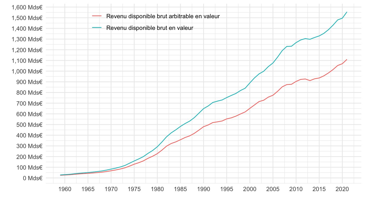
`CNA-2014-RDB` |>
  filter(INDICATEUR %in% c("CNA_B6", "CNA_B6ARBITR")) |>

  year_to_date() |>
  select(INDICATEUR, INDICATEUR, date,  OBS_VALUE) |>
  ggplot() + geom_line(aes(x = date, y = OBS_VALUE, color = INDICATEUR)) +
  theme_minimal() +  xlab("") + ylab("") +

  scale_x_date(breaks = as.Date(paste0(seq(1940, 2020, 5), "-01-01")),
               labels = date_format("%Y")) +
  theme(legend.position = c(0.35, 0.9),
        legend.title = element_blank()) +
  scale_y_log10(breaks = seq(0, 7000, 100),
                     labels = dollar_format(suffix = " Mds€", prefix = "", accuracy = 1))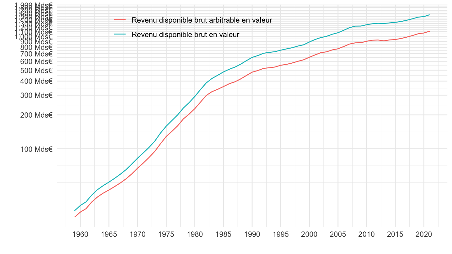
`CNA-2014-RDB` |>
  filter(INDICATEUR %in% c("CNA_B6", "CNA_B6ARBITR")) |>

  year_to_date() |>
  filter(date >= as.Date("1990-01-01")) |>
  group_by(INDICATEUR) |>
  arrange(date) |>
  mutate(index = 100*OBS_VALUE/OBS_VALUE[1]) |>
  ggplot() + geom_line(aes(x = date, y = index, color = INDICATEUR)) +
  xlab("") + ylab("") + theme_minimal() +

  scale_x_date(breaks = as.Date(paste0(seq(1990, 2100, 5), "-01-01")),
               labels = date_format("%Y")) +
  theme(legend.position = c(0.3, 0.85),
        legend.title = element_blank()) +
  scale_y_log10(breaks = seq(100, 300, 5)) +
  geom_label(data = . %>% filter(date == max(date)),
             aes(x = date, y = index, color = INDICATEUR, label = round(index, 1)))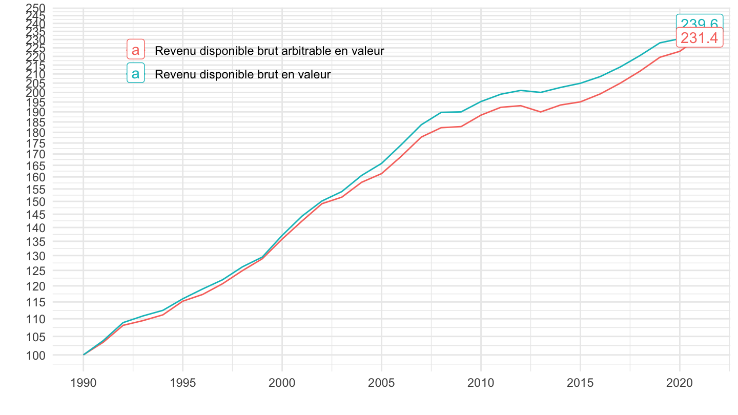
`CNA-2014-RDB` |>
  filter(INDICATEUR %in% c("CNA_B6", "CNA_B6ARBITR")) |>

  year_to_date() |>
  filter(date >= as.Date("1999-01-01")) |>
  group_by(INDICATEUR) |>
  arrange(date) |>
  mutate(index = 100*OBS_VALUE/OBS_VALUE[1]) |>
  ggplot() + geom_line(aes(x = date, y = index, color = INDICATEUR)) +
  xlab("") + ylab("") + theme_minimal() +

  scale_x_date(breaks = as.Date(paste0(seq(1999, 2100, 5), "-01-01")),
               labels = date_format("%Y")) +
  theme(legend.position = c(0.3, 0.85),
        legend.title = element_blank()) +
  scale_y_log10(breaks = seq(100, 300, 5)) +
  geom_label(data = . %>% filter(date == max(date)),
             aes(x = date, y = index, color = INDICATEUR, label = round(index, 1)))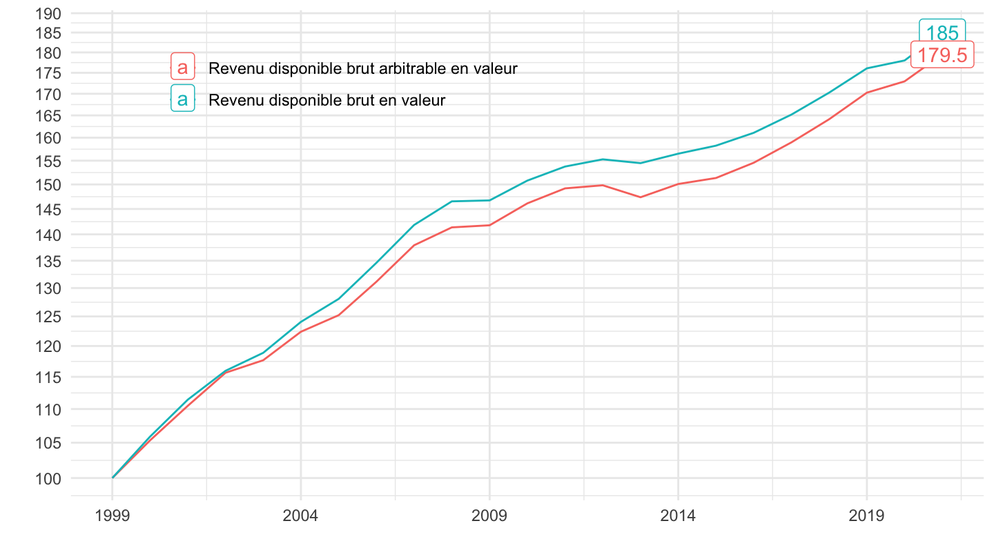
`CNA-2014-RDB` |>
  filter(INDICATEUR %in% c("CNA_B6EVOL", "CNA_B6ARBITREVOL",
                           "CNA_EVOPA", "CNA_EVOPAAR")) |>

  year_to_date() |>
  mutate(OBS_VALUE = OBS_VALUE / 100) |>
  ggplot() + geom_line(aes(x = date, y = OBS_VALUE, color = INDICATEUR)) +
  xlab("") + ylab("") + theme_minimal() +
  scale_x_date(breaks = as.Date(paste0(seq(1940, 2020, 5), "-01-01")),
               labels = date_format("%Y")) +
  theme(legend.position = c(0.7, 0.85),
        legend.title = element_blank()) +
  scale_y_continuous(breaks = 0.01*seq(-2, 90, 2),
                     labels = scales::percent_format(accuracy = 1)) +
  geom_hline(yintercept = 0, linetype = "dashed")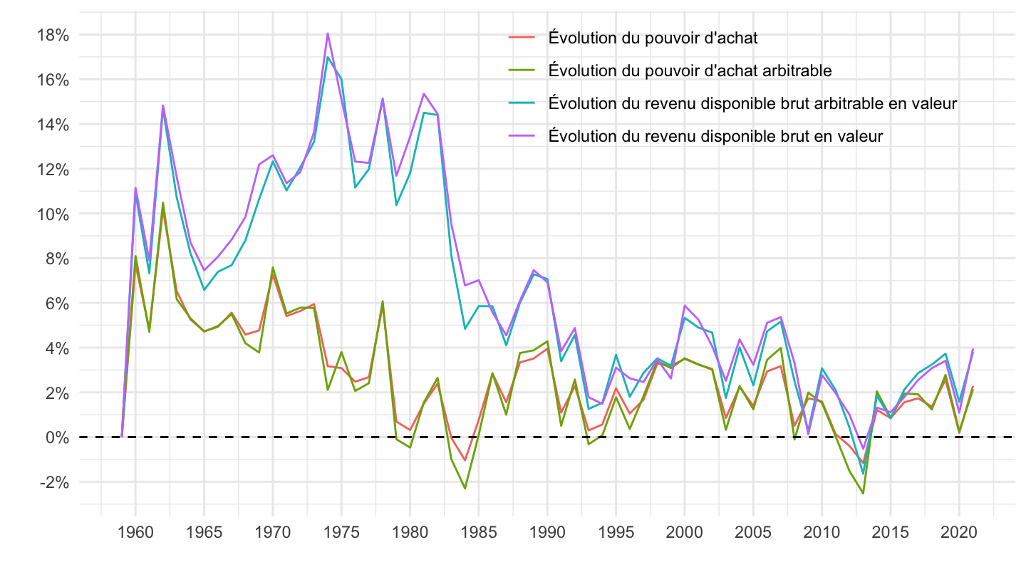
`CNA-2014-RDB` |>
  filter(INDICATEUR %in% c("CNA_EVOPAMEN", "CNA_EVOPAPP",
                           "CNA_EVOPAUC")) |>

  year_to_date() |>
  mutate(OBS_VALUE = OBS_VALUE / 100) |>
  ggplot() + geom_line(aes(x = date, y = OBS_VALUE, color = INDICATEUR)) +
  xlab("") + ylab("Evolution du pouvoir d'achat (%)") + theme_minimal() +

  scale_x_date(breaks = as.Date(paste0(seq(1940, 2020, 5), "-01-01")),
               labels = date_format("%Y")) +
  theme(legend.position = c(0.7, 0.85),
        legend.title = element_blank()) +
  scale_y_continuous(breaks = 0.01*seq(-5, 90, 1),
                     labels = scales::percent_format(accuracy = 1)) +
  geom_hline(yintercept = 0, linetype = "dashed")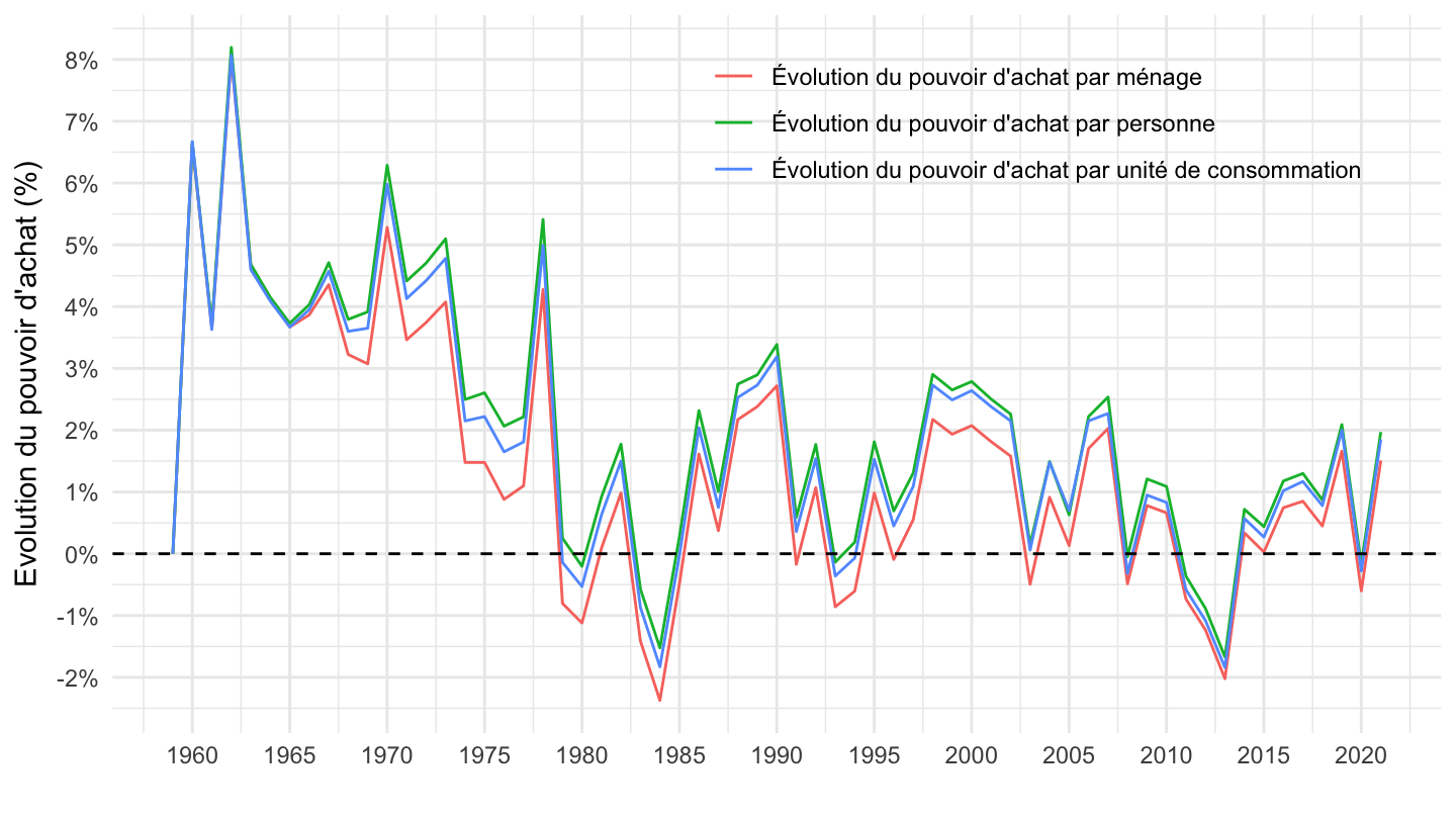
`CNA-2014-RDB` |>
  filter(INDICATEUR %in% c("CNA_EVOPAARMEN", "CNA_EVOPAARPP",
                           "CNA_EVOPAARUC")) |>

  year_to_date() |>
  mutate(OBS_VALUE = OBS_VALUE / 100) |>
  ggplot() + geom_line(aes(x = date, y = OBS_VALUE, color = INDICATEUR)) +
  xlab("") + ylab("Evolution du pouvoir d'achat arbitrable (%)") + theme_minimal() +

  scale_x_date(breaks = as.Date(paste0(seq(1940, 2020, 5), "-01-01")),
               labels = date_format("%Y")) +
  theme(legend.position = c(0.7, 0.85),
        legend.title = element_blank()) +
  scale_y_continuous(breaks = 0.01*seq(-5, 90, 1),
                     labels = scales::percent_format(accuracy = 1)) +
  geom_hline(yintercept = 0, linetype = "dashed")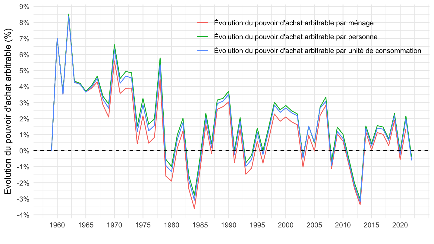
`CNA-2014-RDB` |>
  filter(INDICATEUR %in% c("CNA_EVOPAARMEN", "CNA_EVOPAARPP",
                           "CNA_EVOPAARUC")) |>

  year_to_date() |>
  mutate(OBS_VALUE = OBS_VALUE / 100) |>
  filter(date >= as.Date("1990-01-01")) |>
  select(date, INDICATEUR, INDICATEUR, OBS_VALUE) |>
  group_by(INDICATEUR) |>
  arrange(date) |>
  mutate(index = c(100, 100*cumprod(1+OBS_VALUE[-1]))) |>
  ggplot() + geom_line(aes(x = date, y = index, color = INDICATEUR)) +
  xlab("") + ylab("Evolution du pouvoir d'achat arbitrable (%)") + theme_minimal() +

  scale_x_date(breaks = as.Date(paste0(seq(1940, 2020, 5), "-01-01")),
               labels = date_format("%Y")) +
  theme(legend.position = c(0.3, 0.85),
        legend.title = element_blank()) +
  scale_y_log10(breaks = seq(100, 150, 5)) +
  geom_label(data = . %>% filter(date == max(date)),
             aes(x = date, y = index, color = INDICATEUR, label = round(index, 1)))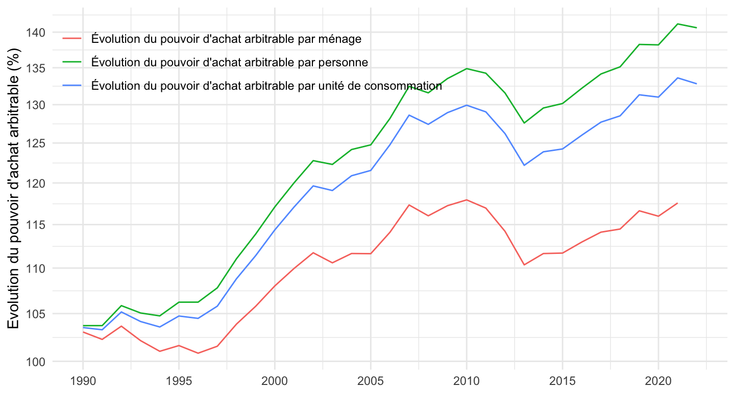
`CNA-2014-RDB` |>
  filter(INDICATEUR %in% c("CNA_EVOPAARMEN", "CNA_EVOPAARPP",
                           "CNA_EVOPAARUC")) |>

  year_to_date() |>
  mutate(OBS_VALUE = OBS_VALUE / 100) |>
  filter(date >= as.Date("1996-01-01")) |>
  select(date, INDICATEUR, INDICATEUR, OBS_VALUE) |>
  group_by(INDICATEUR) |>
  arrange(date) |>
  mutate(index = c(100, 100*cumprod(1+OBS_VALUE[-1]))) |>
  ggplot() + geom_line(aes(x = date, y = index, color = INDICATEUR)) +
  xlab("") + ylab("Evolution du pouvoir d'achat arbitrable (%)") + theme_minimal() +

  scale_x_date(breaks = as.Date(paste0(seq(1996, 2100, 2), "-01-01")),
               labels = date_format("%Y")) +
  theme(legend.position = c(0.3, 0.85),
        legend.title = element_blank()) +
  scale_y_log10(breaks = seq(100, 150, 5)) +
  geom_label(data = . %>% filter(date == max(date)),
             aes(x = date, y = index, color = INDICATEUR, label = round(index, 1)))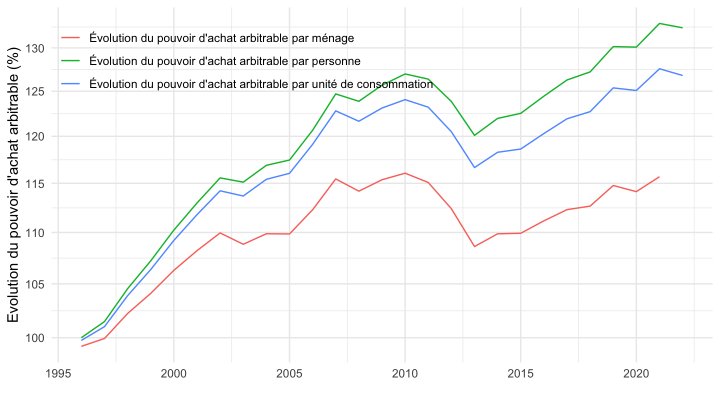
`CNA-2014-RDB` |>
  filter(INDICATEUR %in% c("CNA_EVOPAARMEN", "CNA_EVOPAARPP",
                           "CNA_EVOPAARUC")) |>

  year_to_date() |>
  mutate(OBS_VALUE = OBS_VALUE / 100) |>
  filter(date >= as.Date("1999-01-01")) |>
  select(date, INDICATEUR, INDICATEUR, OBS_VALUE) |>
  group_by(INDICATEUR) |>
  arrange(date) |>
  mutate(index = c(100, 100*cumprod(1 + OBS_VALUE[-1]))) |>
  ggplot() + geom_line(aes(x = date, y = index, color = INDICATEUR)) +
  xlab("") + ylab("Evolution du pouvoir d'achat arbitrable (%)") + theme_minimal() +

  scale_x_date(breaks = as.Date(paste0(seq(1999, 2100, 5), "-01-01")),
               labels = date_format("%Y")) +
  theme(legend.position = c(0.3, 0.85),
        legend.title = element_blank()) +
  scale_y_log10(breaks = seq(100, 150, 5)) +
  geom_label(data = . %>% filter(date == max(date)),
             aes(x = date, y = index, color = INDICATEUR, label = round(index, 1)))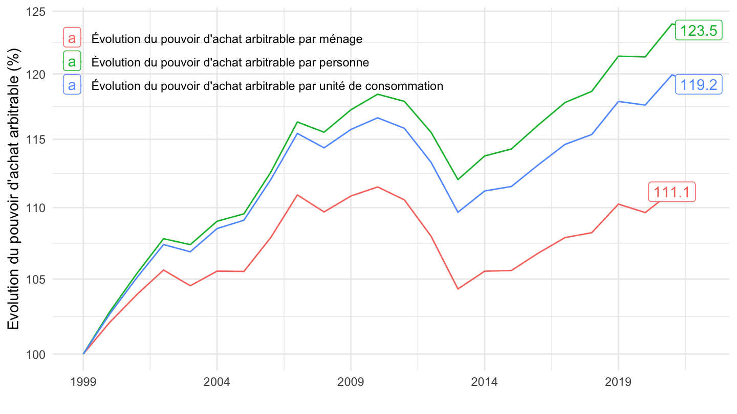
`CNA-2014-RDB` |>
  filter(INDICATEUR %in% c("CNA_EVOPA", "CNA_EVOPAMEN",
                           "CNA_EVOPAUC", "CNA_EVOPAPP")) |>

  year_to_date() |>
  mutate(OBS_VALUE = OBS_VALUE / 100) |>
  filter(date >= as.Date("1990-01-01")) |>
  select(date, INDICATEUR, INDICATEUR, OBS_VALUE) |>
  group_by(INDICATEUR) |>
  arrange(date) |>
  mutate(index = c(100, 100*cumprod(1+OBS_VALUE[-1]))) |>
  ggplot() + geom_line(aes(x = date, y = index, color = INDICATEUR)) +
  xlab("") + ylab("Evolution du pouvoir d'achat arbitrable (%)") + theme_minimal() +

  scale_x_date(breaks = as.Date(paste0(seq(1940, 2020, 5), "-01-01")),
               labels = date_format("%Y")) +
  theme(legend.position = c(0.3, 0.85),
        legend.title = element_blank()) +
  scale_y_log10(breaks = seq(100, 300, 5)) +
  geom_label(data = . %>% filter(date == max(date)),
             aes(x = date, y = index, color = INDICATEUR, label = round(index, 1)))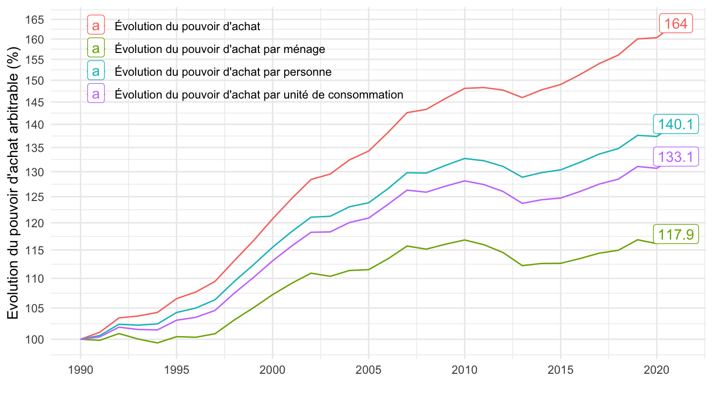
`CNA-2014-RDB` |>
  filter(INDICATEUR %in% c("CNA_EVOPA", "CNA_EVOPAMEN",
                           "CNA_EVOPAUC", "CNA_EVOPAPP")) |>

  year_to_date() |>
  mutate(OBS_VALUE = OBS_VALUE / 100) |>
  filter(date >= as.Date("1996-01-01")) |>
  select(date, INDICATEUR, INDICATEUR, OBS_VALUE) |>
  group_by(INDICATEUR) |>
  arrange(date) |>
  mutate(index = c(100, 100*cumprod(1+OBS_VALUE[-1]))) |>
  ggplot() + geom_line(aes(x = date, y = index, color = INDICATEUR)) +
  xlab("") + ylab("Evolution du pouvoir d'achat arbitrable (%)") + theme_minimal() +

  scale_x_date(breaks = as.Date(paste0(seq(1996, 2100, 2), "-01-01")),
               labels = date_format("%Y")) +
  theme(legend.position = c(0.3, 0.85),
        legend.title = element_blank()) +
  scale_y_log10(breaks = seq(100, 150, 5)) +
  geom_label(data = . %>% filter(date == max(date)),
             aes(x = date, y = index, color = INDICATEUR, label = round(index, 1)))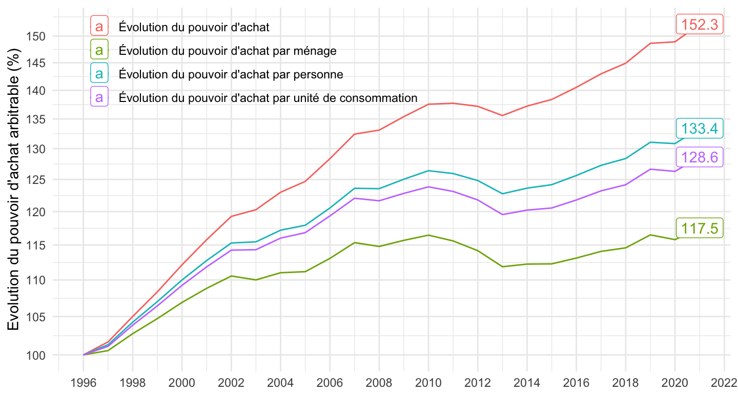
`CNA-2014-RDB` |>
  filter(INDICATEUR %in% c("CNA_EVOPA", "CNA_EVOPAMEN",
                           "CNA_EVOPAUC", "CNA_EVOPAPP")) |>

  year_to_date() |>
  mutate(OBS_VALUE = OBS_VALUE / 100) |>
  filter(date >= as.Date("1999-01-01")) |>
  select(date, INDICATEUR, INDICATEUR, OBS_VALUE) |>
  group_by(INDICATEUR) |>
  arrange(date) |>
  mutate(index = c(100, 100*cumprod(1 + OBS_VALUE[-1]))) |>
  ggplot() + geom_line(aes(x = date, y = index, color = INDICATEUR)) +
  xlab("") + ylab("Evolution du pouvoir d'achat arbitrable (%)") + theme_minimal() +

  scale_x_date(breaks = as.Date(paste0(seq(1999, 2100, 5), "-01-01")),
               labels = date_format("%Y")) +
  theme(legend.position = c(0.3, 0.85),
        legend.title = element_blank()) +
  scale_y_log10(breaks = seq(100, 150, 5)) +
  geom_label(data = . %>% filter(date == max(date)),
             aes(x = date, y = index, color = INDICATEUR, label = round(index, 1)))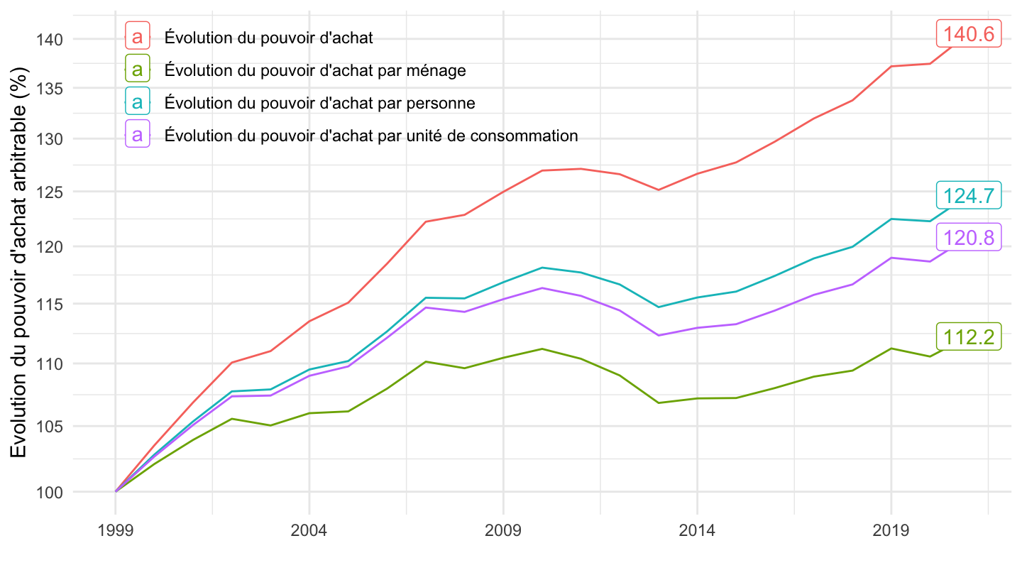
| source | dataset | Title | Updated |
|---|---|---|---|
| source | dataset | Title | Updated |
|---|---|---|---|


