2.104 – Compte des ménages simplifié et ratios d’épargne (En milliards d’euros et %) - t_2104_2018

Data - INSEE

Author

Code

load_data("insee/t_2104_2018_old.RData")
load_data("insee/CNA-2014-PIB.RData")
load_data("us/nber_recessions.RData")

Organisation

Revenu et pouvoir d’achat des ménages en 2018. html

variable

Code

t_2104_2018 %>%
  group_by(line, Line) %>%
  summarise(Nobs = n()) %>%
  {if (is_html_output()) datatable(., filter = 'top', rownames = F) else .}

gdp

Code

gdp <- `CNA-2014-PIB` %>%
  yearend_to_date %>%
  filter(OPERATION == "PIB",
         UNIT_MEASURE %in% c("EUROS_COURANTS")) %>%
  mutate(value = (OBS_VALUE %>% as.numeric)/1000,
         variable = paste0("PIB_", UNIT_MEASURE),
         variable_desc = "Produit Intérieur Brut") %>%
  select(date, value)

Code

gdp %>%
  mutate(value = round(value) %>% paste0(" Mds€")) %>%
  {if (is_html_output()) datatable(., filter = 'top', rownames = F) else .}

Ex 1: Table in 2018

Code

t_2104_2018 %>%
  filter(date == as.Date("2018-12-31")) %>%
  select(-date) %>%
  mutate(value = round(value) %>% paste0(" Mds€")) %>%
  {if (is_html_output()) datatable(., filter = 'top', rownames = F) else .}

Ex: Rémunération des salariés

Code

t_2104_2018 %>%
  group_by(date) %>%
  mutate(value = value/value[line == 18]) %>%
  filter(line %in% c(5, 4)) %>%
  ggplot(.) + theme_minimal() + 
  geom_line(aes(x = date, y = value, color = Line, linetype = Line)) +
  theme(legend.title = element_blank(),
        legend.position = c(0.3, 0.9)) +
  geom_rect(data = nber_recessions %>%
              filter(Peak > as.Date("1949-01-01")), 
            aes(xmin = Peak, xmax = Trough, ymin = -Inf, ymax = +Inf), 
            fill = 'grey', alpha = 0.5) + 
  scale_x_date(breaks = seq(1950, 2020, 5) %>% paste0("-01-01") %>% as.Date,
               limits = c(1949, 2020) %>% paste0("-01-01") %>% as.Date,
               labels = date_format("%y")) +
  ylab("% du RDBA") + xlab("") +
  scale_color_manual(values = viridis(5)[1:4]) +
  scale_y_continuous(breaks = 0.01*seq(0, 100, 5),
                     labels = scales::percent_format(accuracy = 1))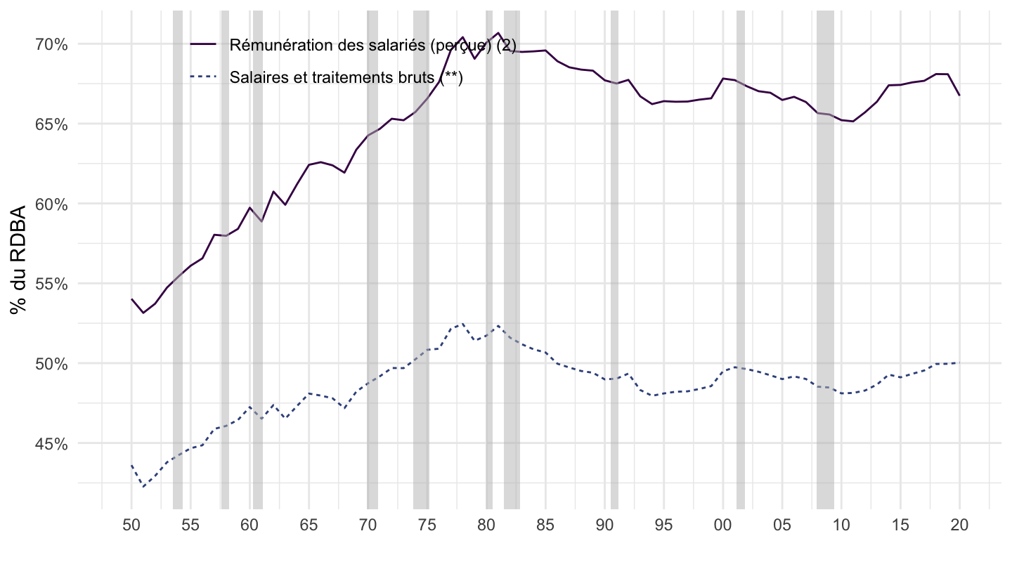

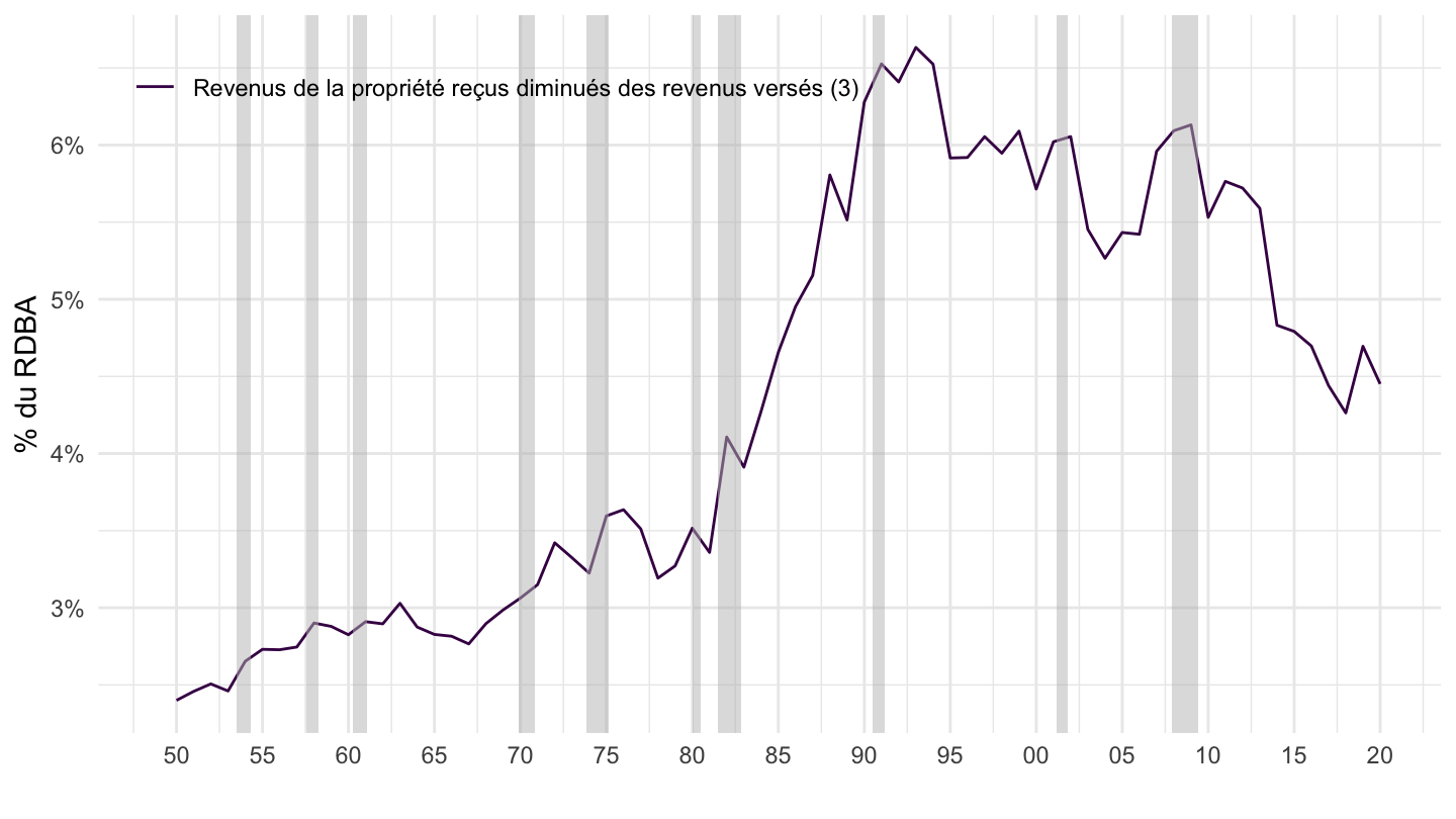
Ex: Loyers, Business

Code

t_2104_2018 %>%
  group_by(date) %>%
  mutate(value = value/value[line == 18]) %>%
  filter(line %in% c(2, 3)) %>%
  ggplot(.) + theme_minimal() + 
  geom_line(aes(x = date, y = value, color = Line, linetype = Line)) +
  theme(legend.title = element_blank(),
        legend.position = c(0.3, 0.9)) +
  geom_rect(data = nber_recessions %>%
              filter(Peak > as.Date("1949-01-01")), 
            aes(xmin = Peak, xmax = Trough, ymin = -Inf, ymax = +Inf), 
            fill = 'grey', alpha = 0.5) + 
  scale_x_date(breaks = seq(1950, 2020, 5) %>% paste0("-01-01") %>% as.Date,
               limits = c(1949, 2020) %>% paste0("-01-01") %>% as.Date,
               labels = date_format("%y")) +
  ylab("% du RDBA") + xlab("") +
  scale_color_manual(values = viridis(5)[1:4]) +
  scale_y_continuous(breaks = 0.01*seq(0, 100, 5),
                     labels = scales::percent_format(accuracy = 1))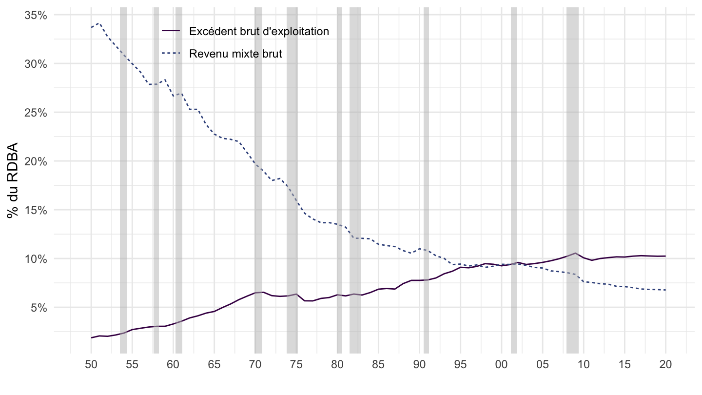

Ex: Revenus de la propriété

Code

t_2104_2018 %>%
  group_by(date) %>%
  mutate(value = value/value[line == 18]) %>%
  filter(line %in% c(9)) %>%
  ggplot(.) + theme_minimal() + 
  geom_line(aes(x = date, y = value, color = Line, linetype = Line)) +
  theme(legend.title = element_blank(),
        legend.position = c(0.3, 0.9)) +
  geom_rect(data = nber_recessions %>%
              filter(Peak > as.Date("1949-01-01")), 
            aes(xmin = Peak, xmax = Trough, ymin = -Inf, ymax = +Inf), 
            fill = 'grey', alpha = 0.5) + 
  scale_x_date(breaks = seq(1950, 2020, 5) %>% paste0("-01-01") %>% as.Date,
               limits = c(1949, 2020) %>% paste0("-01-01") %>% as.Date,
               labels = date_format("%y")) +
  ylab("% du RDBA") + xlab("") +
  scale_color_manual(values = viridis(5)[1:4]) +
  scale_y_continuous(breaks = 0.01*seq(0, 100, 1),
                     labels = scales::percent_format(accuracy = 1))