Équilibre du produit intérieur brut
Données - INSEE
Info
Last observation: 2024-Q1
First observation: 1949-Q1
Number of observations: 20 236
Last data update: 24 jul 2026, 01:15. Last compile: 24 jul 2026, 05:36
Structure
Info
Données sur la macroéconomie en France
| source | dataset | Title | .html | .rData |
|---|---|---|---|---|
| insee | CNT-2014-PIB-EQB-RF | Équilibre du produit intérieur brut | 2026-07-23 | 2026-07-23 |
| bdf | CFT | Comptes Financiers Trimestriels | 2026-07-23 | 2025-03-09 |
| insee | CNA-2014-CONSO-SI | Dépenses de consommation finale par secteur institutionnel | 2026-07-23 | 2026-07-23 |
| insee | CNA-2014-CSI | Comptes des secteurs institutionnels | 2026-07-23 | 2026-07-23 |
| insee | CNA-2014-FBCF-BRANCHE | Formation brute de capital fixe (FBCF) par branche | 2026-07-23 | 2026-07-23 |
| insee | CNA-2014-FBCF-SI | Formation brute de capital fixe (FBCF) par secteur institutionnel | 2026-07-23 | 2026-07-23 |
| insee | CNA-2014-RDB | Revenu et pouvoir d’achat des ménages | 2026-07-23 | 2026-07-23 |
| insee | CNA-2020-CONSO-MEN | Consommation des ménages | 2026-07-23 | 2026-07-23 |
| insee | CNA-2020-PIB | Produit intérieur brut (PIB) et ses composantes | 2026-07-23 | 2026-07-23 |
| insee | CNT-2014-CB | Comptes des branches | 2026-07-23 | 2026-07-23 |
| insee | CNT-2014-CSI | Comptes de secteurs institutionnels | 2026-07-23 | 2026-07-22 |
| insee | CNT-2014-OPERATIONS | Opérations sur biens et services | 2026-07-23 | 2026-07-23 |
| insee | CONSO-MENAGES-2020 | Consommation des ménages en biens | 2026-07-23 | 2026-07-23 |
| insee | ICA-2015-IND-CONS | Indices de chiffre d'affaires dans l'industrie et la construction | 2026-07-23 | 2026-07-23 |
| insee | conso-mensuelle | Consommation de biens, données mensuelles | 2026-07-23 | 2023-07-04 |
| insee | t_1101 | 1.101 – Le produit intérieur brut et ses composantes à prix courants (En milliards d'euros) | 2026-07-23 | 2022-01-02 |
| insee | t_1102 | 1.102 – Le produit intérieur brut et ses composantes en volume aux prix de l'année précédente chaînés (En milliards d'euros 2014) | 2026-07-23 | 2020-10-30 |
| insee | t_1105 | 1.105 – Produit intérieur brut - les trois approches à prix courants (En milliards d'euros) - t_1105 | 2026-07-23 | 2020-10-30 |
LAST_COMPILE
| LAST_COMPILE |
|---|
| 2026-07-24 |
Last
Code
`CNT-2014-PIB-EQB-RF` %>%
  filter(TIME_PERIOD == max(TIME_PERIOD)) %>%
  select(TIME_PERIOD, TITLE_FR, OBS_VALUE) %>%
  print_table_conditional()
Last - 2022-Q1
Tous
Code
`CNT-2014-PIB-EQB-RF` %>%
  filter(TIME_PERIOD == "2022-Q1") %>%
  select_if(~ n_distinct(.) > 1) %>%
  select(-IDBANK, -TITLE_EN) %>%
  arrange(-OBS_VALUE) %>%
  print_table_conditional
% du PIB
Code
`CNT-2014-PIB-EQB-RF` %>%
  filter(FREQ == "T",
         VALORISATION == "V",
         TIME_PERIOD == "2022-Q1") %>%
  select_if(~ n_distinct(.) > 1) %>%
  select(-IDBANK, -TITLE_EN) %>%
  arrange(-OBS_VALUE) %>%
  mutate(`% of GDP` = round(100*OBS_VALUE/OBS_VALUE[OPERATION == "PIB"], 1)) %>%
print_table_conditional| OPERATION | SECT-INST | CNA_PRODUIT | TITLE_FR | OBS_VALUE | OBS_REV | Operation | Sect-Inst | % of GDP |
|---|---|---|---|---|---|---|---|---|
| DINTF | SO | SO | Demande intérieure totale finale - Valeur aux prix courants - Série CVS-CJO - Série arrêtée | 664069 | 1 | Demande intérieure totale finale | Sans objet | 103.0 |
| DINTFHS | SO | SO | Demande intérieure totale finale hors stocks - Valeur aux prix courants - Série CVS-CJO - Série arrêtée | 656929 | 1 | Demande intérieure totale finale hors stocks | Sans objet | 101.9 |
| PIB | SO | SO | Produit intérieur brut total - Valeur aux prix courants - Série CVS-CJO - Série arrêtée | 644543 | 1 | PIB - Produit intérieur brut | Sans objet | 100.0 |
| P4 | SO | D-CNT | Dépenses de consommation totales - Valeur aux prix courants - Série CVS-CJO - Série arrêtée | 497031 | 1 | P4 - Consommation finale effective | Sans objet | 77.1 |
| P3 | S14 | D-CNT | Dépenses de consommation des ménages - Total - Valeur aux prix courants - Série CVS-CJO - Série arrêtée | 326685 | 1 | P3 - Dépense de consommation finale | S14 - Ménages y compris entreprises individuelles | 50.7 |
| P7 | SO | D-CNT | Importations - Total - Valeur aux prix courants - Série CVS-CJO - Série arrêtée | 236170 | 1 | P7 - Importations de biens et services | Sans objet | 36.6 |
| P6 | SO | D-CNT | Exportations - Total - Valeur aux prix courants - Série CVS-CJO - Série arrêtée | 216644 | 1 | P6 - Exportations de biens et services | Sans objet | 33.6 |
| P51 | S0 | D-CNT | FBCF de l'ensemble des secteurs institutionnels - Total - Valeur aux prix courants - Série CVS-CJO - Série arrêtée | 159898 | 1 | P51 - Formation brute de capital fixe | S0 - Ensemble des secteurs institutionnels | 24.8 |
| P3 | SO | SO | Dépenses de consommation des APU - Total - Valeur aux prix courants - Série CVS-CJO - Série arrêtée | 156513 | 1 | P3 - Dépense de consommation finale | Sans objet | 24.3 |
| P31 | SO | D-CNT | Dépenses de consommation individualisable des APU - Total - Valeur aux prix courants - Série CVS-CJO - Série arrêtée | 103457 | 1 | P31 - Dépense de consommation finale individuelle | Sans objet | 16.1 |
| P51S | S11 | D-CNT | Investissement des entreprises non financières - Total - Valeur aux prix courants - Série CVS-CJO - Série arrêtée | 88982 | 1 | P51S - FBCF des entreprises non financières (y compris entreprises individuelles) | S11 - Sociétés non financières | 13.8 |
| P32 | SO | D-CNT | Dépenses de consommation collective des APU - Total - Valeur aux prix courants - Série CVS-CJO - Série arrêtée | 53056 | 1 | P32 - Dépense de consommation finale collective | Sans objet | 8.2 |
| D211 | SO | D-CNT | TVA - Total - Valeur aux prix courants - Série CVS-CJO - Série arrêtée | 48828 | 1 | D211 - Impôts de type 'Taxe à la Valeur Ajoutée' (TVA) | Sans objet | 7.6 |
| P51M | S14 | D-CNT | FBCF des ménages - Total - Valeur aux prix courants - Série CVS-CJO - Série arrêtée | 38523 | 1 | P51M - FBCF des ménages (hors entreprises individuelles) | S14 - Ménages y compris entreprises individuelles | 6.0 |
| D214 | SO | D-CNT | Autres impôts sur les produits - Total - Valeur aux prix courants - Série CVS-CJO - Série arrêtée | 29146 | 1 | D214 - Autres impôts sur les produits | Sans objet | 4.5 |
| P51G | S13 | D-CNT | FBCF des administrations publiques - Total - Valeur aux prix courants - Série CVS-CJO - Série arrêtée | 23749 | 1 | P51G - Formation brute de capital fixe | S13 - Administrations publiques (APU) | 3.7 |
| P3 | S15 | D-CNT | Dépenses de consommation des ISBLSM - Total - Valeur aux prix courants - Série CVS-CJO - Série arrêtée | 13833 | NA | P3 - Dépense de consommation finale | S15 - Institutions sans but lucratif au service des ménages | 2.1 |
| P51B | S12 | D-CNT | FBCF des sociétés financières - Total - Valeur aux prix courants - Série CVS-CJO - Série arrêtée | 7292 | 1 | P51B - FBCF des entreprises financières (y compris entreprises individuelles) | S12 - Sociétés financières | 1.1 |
| P54 | SO | D-CNT | Stocks et acquisitions moins cessions d'objets de valeur - Total - Valeur aux prix courants - Série CVS-CJO - Série arrêtée | 7139 | 1 | P54 - Stocks et acquisitions moins cession d'objets de valeur | Sans objet | 1.1 |
| P52 | SO | D-CNT | Variation des stocks - Total - Valeur aux prix courants - Série CVS-CJO - Série arrêtée | 6789 | 1 | P52 - Variation de stocks | Sans objet | 1.1 |
| P51P | S15 | D-CNT | FBCF des ISBLSM - Total - Valeur aux prix courants - Série CVS-CJO - Série arrêtée | 1352 | NA | P51P - FBCF des ISBLSM | S15 - Institutions sans but lucratif au service des ménages | 0.2 |
| D212 | SO | D-CNT | Impôts sur importations - Total - Valeur aux prix courants - Série CVS-CJO - Série arrêtée | 915 | 1 | D212 - Impôts sur les importations autres que la taxe à la valeur ajoutée | Sans objet | 0.1 |
| P53 | SO | D-CNT | Acquisitions moins cessions d'objets de valeur - Total - Valeur aux prix courants - Série CVS-CJO - Série arrêtée | 351 | NA | P53 - Acquisitions moins cession d'objets de valeur | Sans objet | 0.1 |
| D319 | SO | D-CNT | Subventions - Total - Valeur aux prix courants - Série CVS-CJO - Série arrêtée | -7753 | NA | D319 - Autres subventions sur les produits | Sans objet | -1.2 |
| SOLDE | SO | SO | Solde extérieur total - Valeur aux prix courants - Série CVS-CJO - Série arrêtée | -19526 | 1 | SOLDE - Solde extérieur total | Sans objet | -3.0 |
Deflators
All
Code
`CNT-2014-PIB-EQB-RF` %>%
  filter(OPERATION %in% c("PIB", "P3", "P4"),
         VALORISATION %in% c("V", "L"),
         NATURE == "VALEUR_ABSOLUE") %>%
  select_if(~ n_distinct(.) > 1) %>%
  select(-IDBANK, -TITLE_EN) %>%
  rowwise() %>%
  mutate(date = TIME_PERIOD_to_date(TIME_PERIOD)) %>%
  arrange(desc(date)) %>%
  group_by(OPERATION, `SECT-INST`, date) %>%
  summarise(deflator = 100*OBS_VALUE[VALORISATION == "V"]/OBS_VALUE[VALORISATION == "L"]) %>%
  ungroup %>%
  left_join(OPERATION, by = "OPERATION") %>%
  left_join(`SECT-INST`, by = "SECT-INST") %>%
  mutate(variable = paste0(OPERATION, " - ", `Sect-Inst`)) %>%
  ggplot + geom_line(aes(x = date, y = deflator, color = variable)) +
  theme_minimal() + xlab("") + ylab("") +
  scale_x_date(breaks = seq(1920, 2100, 5) %>% paste0("-01-01") %>% as.Date,
               labels = date_format("%Y")) +
  scale_y_log10() +
  theme(legend.position = c(0.5, 0.8),
        legend.title = element_blank())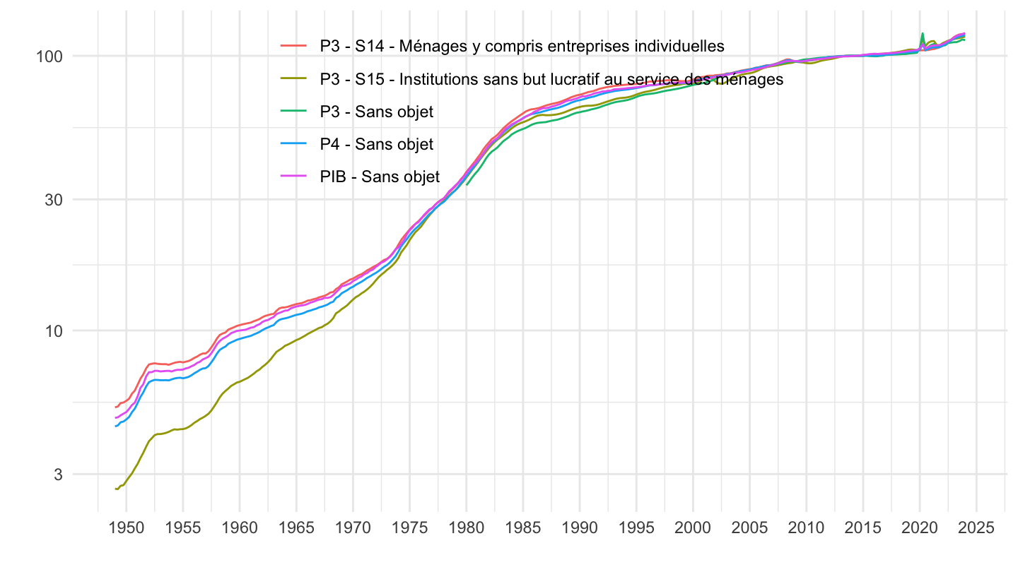
2014-
Code
`CNT-2014-PIB-EQB-RF` %>%
  filter(OPERATION %in% c("PIB", "P3", "P4"),
         VALORISATION %in% c("V", "L"),
         NATURE == "VALEUR_ABSOLUE") %>%
  select_if(~ n_distinct(.) > 1) %>%
  select(-IDBANK, -TITLE_EN) %>%
  rowwise() %>%
  mutate(date = TIME_PERIOD_to_date(TIME_PERIOD)) %>%
  arrange(desc(date)) %>%
  group_by(OPERATION, `SECT-INST`, date) %>%
  summarise(deflator = 100*OBS_VALUE[VALORISATION == "V"]/OBS_VALUE[VALORISATION == "L"]) %>%
  ungroup %>%
  left_join(OPERATION, by = "OPERATION") %>%
  left_join(`SECT-INST`, by = "SECT-INST") %>%
  filter(date >= as.Date("2014-01-01")) %>%
  mutate(variable = paste0(OPERATION, " - ", `Sect-Inst`)) %>%
  ggplot + geom_line(aes(x = date, y = deflator, color = variable)) +
  theme_minimal() + xlab("") + ylab("") +
  scale_x_date(breaks = seq(1920, 2100, 1) %>% paste0("-01-01") %>% as.Date,
               labels = date_format("%Y")) +
  scale_y_log10() +
  theme(legend.position = c(0.5, 0.8),
        legend.title = element_blank())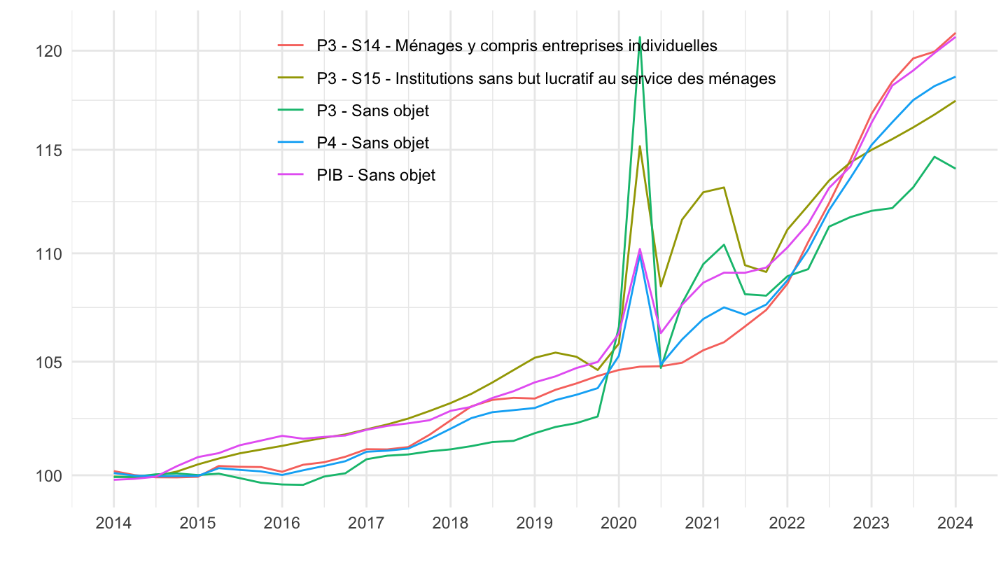
2019-
Code
`CNT-2014-PIB-EQB-RF` %>%
  filter(OPERATION %in% c("PIB", "P3", "P4"),
         VALORISATION %in% c("V", "L"),
         NATURE == "VALEUR_ABSOLUE") %>%
  select_if(~ n_distinct(.) > 1) %>%
  select(-IDBANK, -TITLE_EN) %>%
  rowwise() %>%
  mutate(date = TIME_PERIOD_to_date(TIME_PERIOD)) %>%
  arrange(desc(date)) %>%
  group_by(OPERATION, `SECT-INST`, date) %>%
  summarise(deflator = 100*OBS_VALUE[VALORISATION == "V"]/OBS_VALUE[VALORISATION == "L"]) %>%
  ungroup %>%
  left_join(OPERATION, by = "OPERATION") %>%
  left_join(`SECT-INST`, by = "SECT-INST") %>%
  filter(date >= as.Date("2019-01-01")) %>%
  mutate(variable = paste0(OPERATION, " - ", `Sect-Inst`)) %>%
  ggplot + geom_line(aes(x = date, y = deflator, color = variable)) +
  theme_minimal() + xlab("") + ylab("") +
  scale_x_date(breaks = seq(1920, 2100, 1) %>% paste0("-01-01") %>% as.Date,
               labels = date_format("%Y")) +
  scale_y_log10() +
  theme(legend.position = c(0.5, 0.8),
        legend.title = element_blank())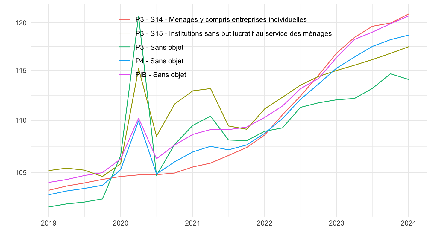
2020-
Code
`CNT-2014-PIB-EQB-RF` %>%
  filter(OPERATION %in% c("PIB", "P3", "P4"),
         VALORISATION %in% c("V", "L"),
         NATURE == "VALEUR_ABSOLUE") %>%
  select_if(~ n_distinct(.) > 1) %>%
  select(-IDBANK, -TITLE_EN) %>%
  rowwise() %>%
  mutate(date = TIME_PERIOD_to_date(TIME_PERIOD)) %>%
  arrange(desc(date)) %>%
  group_by(OPERATION, `SECT-INST`, date) %>%
  summarise(deflator = 100*OBS_VALUE[VALORISATION == "V"]/OBS_VALUE[VALORISATION == "L"]) %>%
  ungroup %>%
  left_join(OPERATION, by = "OPERATION") %>%
  left_join(`SECT-INST`, by = "SECT-INST") %>%
  filter(date >= as.Date("2020-01-01")) %>%
  mutate(variable = paste0(OPERATION, " - ", `Sect-Inst`)) %>%
  ggplot + geom_line(aes(x = date, y = deflator, color = variable)) +
  theme_minimal() + xlab("") + ylab("") +
  scale_x_date(breaks = seq(1920, 2100, 1) %>% paste0("-01-01") %>% as.Date,
               labels = date_format("%Y")) +
  scale_y_log10() +
  theme(legend.position = c(0.5, 0.8),
        legend.title = element_blank())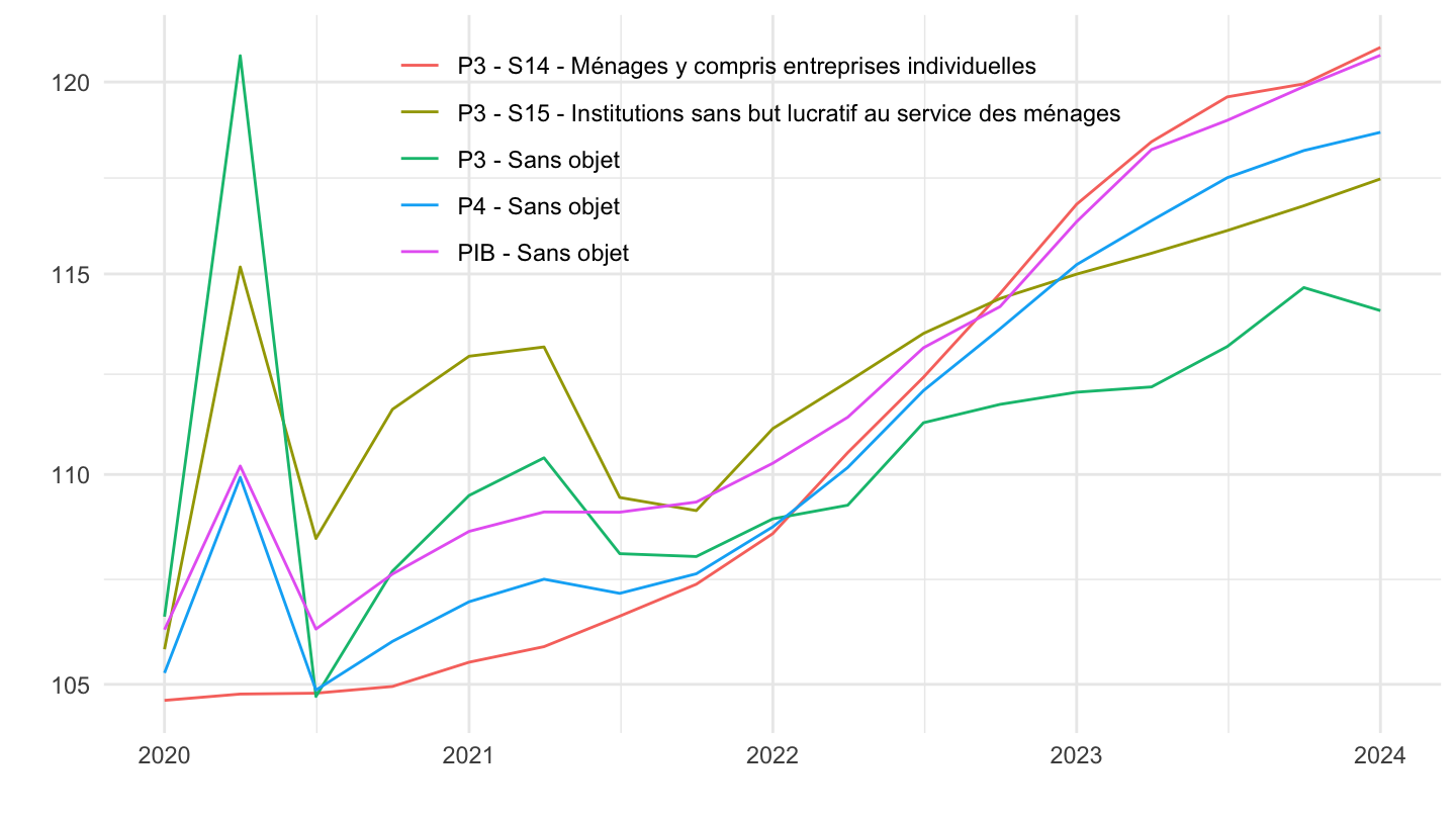
2021-
Code
`CNT-2014-PIB-EQB-RF` %>%
  filter(OPERATION %in% c("PIB", "P3", "P4"),
         VALORISATION %in% c("V", "L"),
         NATURE == "VALEUR_ABSOLUE") %>%
  select_if(~ n_distinct(.) > 1) %>%
  select(-IDBANK, -TITLE_EN) %>%
  rowwise() %>%
  mutate(date = TIME_PERIOD_to_date(TIME_PERIOD)) %>%
  arrange(desc(date)) %>%
  group_by(OPERATION, `SECT-INST`, date) %>%
  summarise(deflator = 100*OBS_VALUE[VALORISATION == "V"]/OBS_VALUE[VALORISATION == "L"]) %>%
  ungroup %>%
  left_join(OPERATION, by = "OPERATION") %>%
  left_join(`SECT-INST`, by = "SECT-INST") %>%
  filter(date >= as.Date("2021-01-01")) %>%
  mutate(variable = paste0(OPERATION, " - ", `Sect-Inst`)) %>%
  group_by(OPERATION, `SECT-INST`) %>%
  mutate(deflator = 100*deflator/deflator[1]) %>%
  ggplot + geom_line(aes(x = date, y = deflator, color = variable)) +
  theme_minimal() + xlab("") + ylab("") +
  scale_x_date(breaks = seq(1920, 2100, 1) %>% paste0("-01-01") %>% as.Date,
               labels = date_format("%Y")) +
  scale_y_log10() +
  theme(legend.position = c(0.5, 0.8),
        legend.title = element_blank())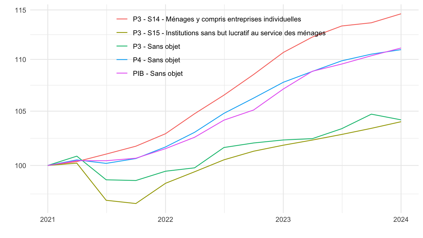
Agrégats
consommation nominale
Code
`CNT-2014-PIB-EQB-RF` %>%
  filter(FREQ == "T",
         VALORISATION == "V",
         OPERATION %in% c("P3", "PIB")) %>%
  quarter_to_date %>%
  filter(date >= as.Date("2022-01-01")) %>%
  group_by(OPERATION, `SECT-INST`) %>%
  arrange(date) %>%
  mutate(OBS_VALUE = OBS_VALUE/OBS_VALUE[1]) %>%
  mutate(TITLE_FR = gsub("- Valeur aux prix courants - Série CVS-CJO", "", TITLE_FR)) %>%
  ggplot() + ylab("% du PIB") + xlab("") + theme_minimal() +
  geom_line(aes(x = date, y = OBS_VALUE, color = TITLE_FR)) +

  scale_x_date(breaks = seq(1920, 2100, 5) %>% paste0("-01-01") %>% as.Date,
               labels = date_format("%Y")) +
  theme(legend.position = c(0.25, 0.4),
        legend.title = element_blank()) +
  scale_y_continuous(breaks = 0.01*seq(0, 300, 5),
                     labels = percent_format(accuracy = 1))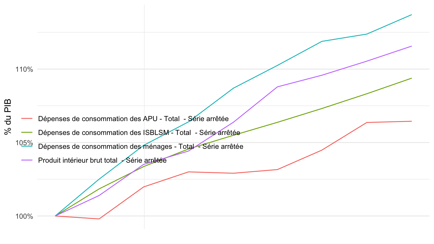
Consommation: P4, P3
All
Code
`CNT-2014-PIB-EQB-RF` %>%
  filter(FREQ == "T",
         VALORISATION == "V",
         OPERATION %in% c("P4", "P3", "PIB")) %>%
  quarter_to_date %>%
  group_by(date) %>%
  mutate(OBS_VALUE = OBS_VALUE/OBS_VALUE[OPERATION == "PIB"]) %>%
  filter(OPERATION != "PIB") %>%
  mutate(TITLE_FR = gsub("- Valeur aux prix courants - Série CVS-CJO", "", TITLE_FR)) %>%
  ggplot() + ylab("% du PIB") + xlab("") + theme_minimal() +
  geom_line(aes(x = date, y = OBS_VALUE, color = TITLE_FR)) +

  scale_x_date(breaks = seq(1920, 2100, 5) %>% paste0("-01-01") %>% as.Date,
               labels = date_format("%Y")) +
  theme(legend.position = c(0.25, 0.4),
        legend.title = element_blank()) +
  scale_y_continuous(breaks = 0.01*seq(0, 300, 5),
                     labels = percent_format(accuracy = 1))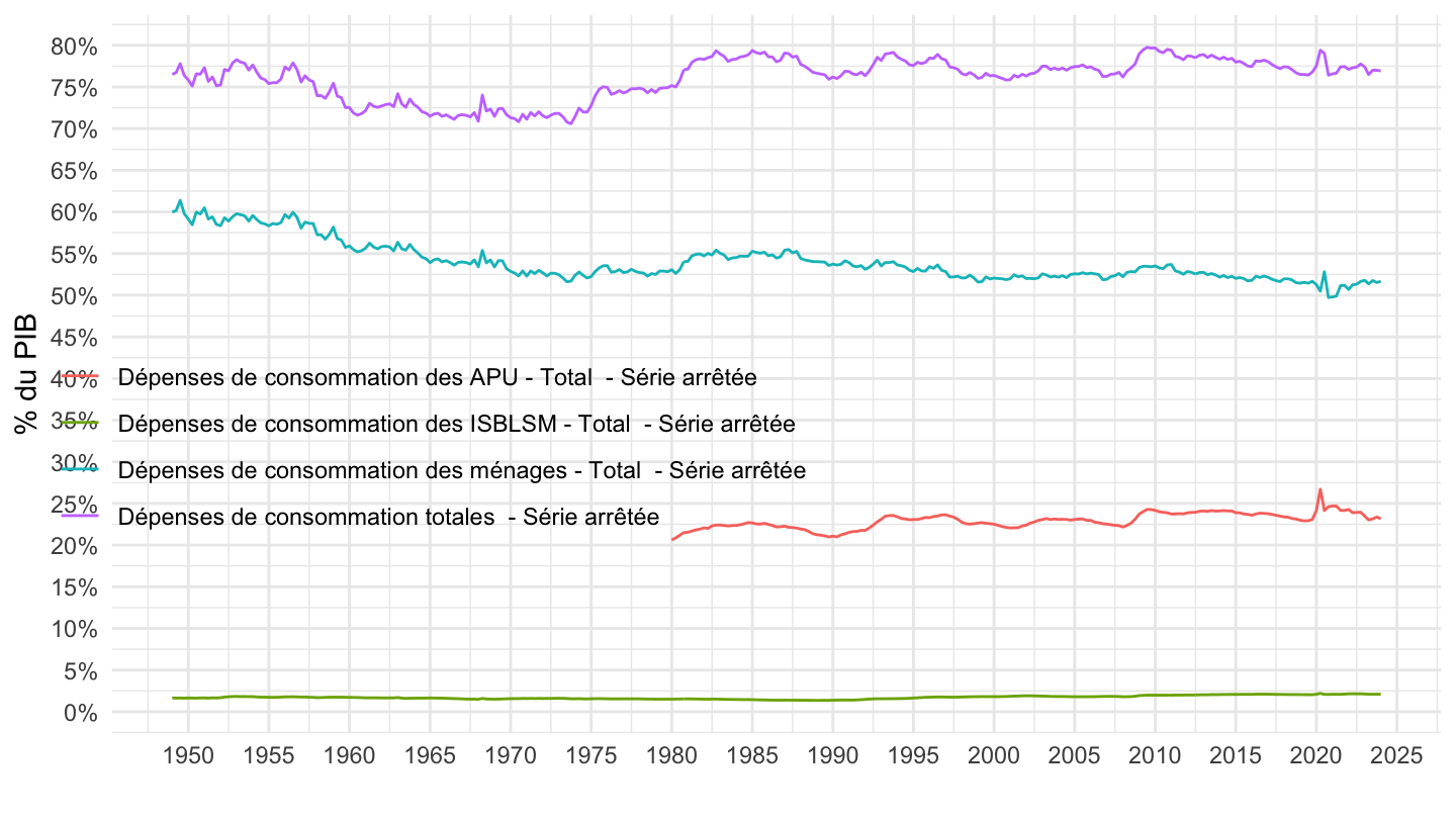
1980-
Code
`CNT-2014-PIB-EQB-RF` %>%
  filter(FREQ == "T",
         VALORISATION == "V",
         OPERATION %in% c("P4", "P3", "PIB")) %>%
  quarter_to_date %>%
  group_by(date) %>%
  mutate(OBS_VALUE = OBS_VALUE/OBS_VALUE[OPERATION == "PIB"]) %>%
  filter(OPERATION != "PIB") %>%
  mutate(TITLE_FR = gsub("- Valeur aux prix courants - Série CVS-CJO", "", TITLE_FR)) %>%
  filter(date >= as.Date("1980-01-01")) %>%
  ggplot() + ylab("% du PIB") + xlab("") + theme_minimal() +
  geom_line(aes(x = date, y = OBS_VALUE, color = TITLE_FR)) +

  scale_x_date(breaks = seq(1920, 2100, 5) %>% paste0("-01-01") %>% as.Date,
               labels = date_format("%Y")) +
  theme(legend.position = c(0.25, 0.4),
        legend.title = element_blank()) +
  scale_y_continuous(breaks = 0.01*seq(0, 300, 5),
                     labels = percent_format(accuracy = 1))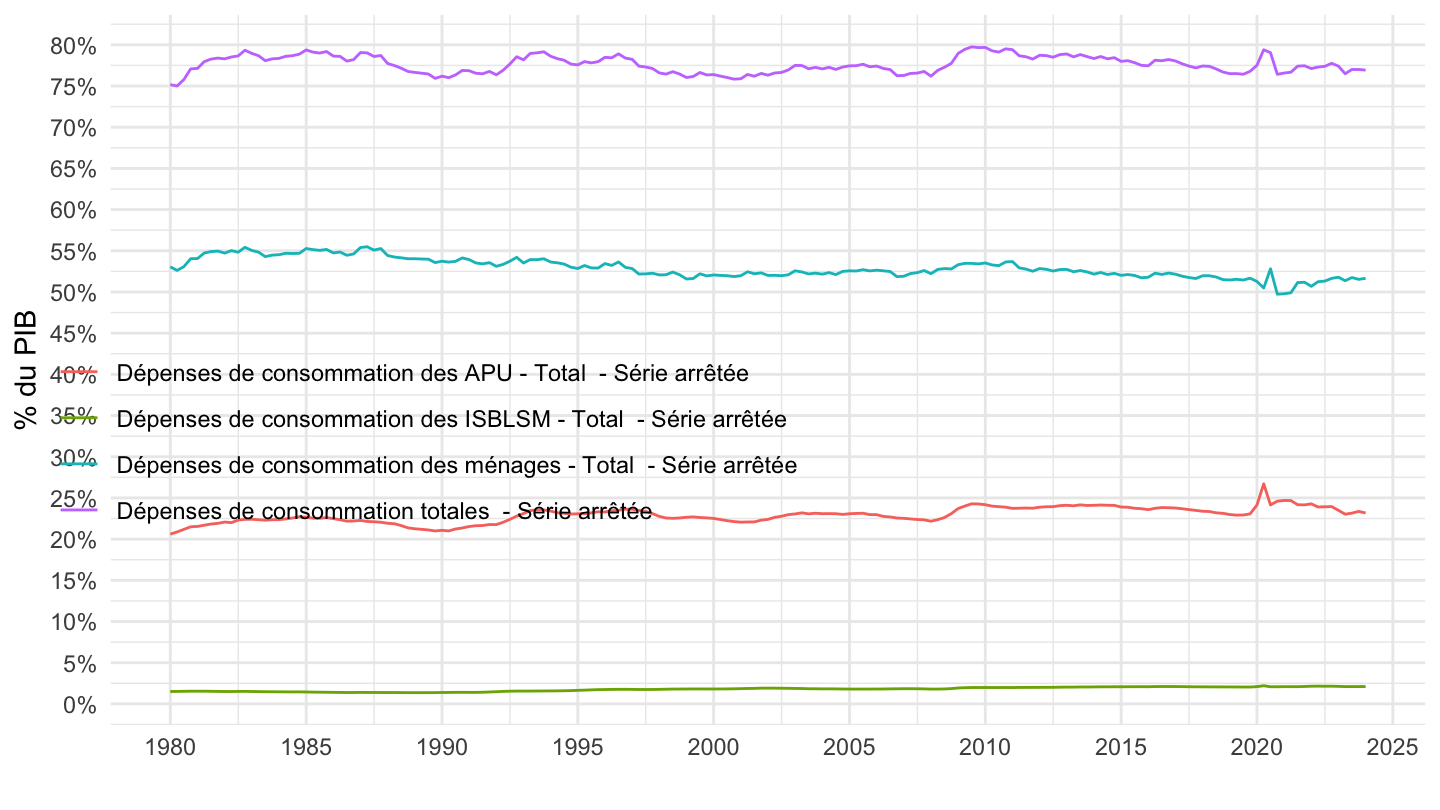
1995-
Code
`CNT-2014-PIB-EQB-RF` %>%
  filter(FREQ == "T",
         VALORISATION == "V",
         OPERATION %in% c("P4", "P3", "PIB")) %>%
  quarter_to_date %>%
  group_by(date) %>%
  mutate(OBS_VALUE = OBS_VALUE/OBS_VALUE[OPERATION == "PIB"]) %>%
  filter(OPERATION != "PIB") %>%
  mutate(TITLE_FR = gsub("- Valeur aux prix courants - Série CVS-CJO", "", TITLE_FR)) %>%
  filter(date >= as.Date("1995-01-01")) %>%
  ggplot() + ylab("% du PIB") + xlab("") + theme_minimal() +
  geom_line(aes(x = date, y = OBS_VALUE, color = TITLE_FR)) +

  scale_x_date(breaks = seq(1920, 2100, 5) %>% paste0("-01-01") %>% as.Date,
               labels = date_format("%Y")) +
  theme(legend.position = c(0.25, 0.4),
        legend.title = element_blank()) +
  scale_y_continuous(breaks = 0.01*seq(0, 300, 5),
                     labels = percent_format(accuracy = 1))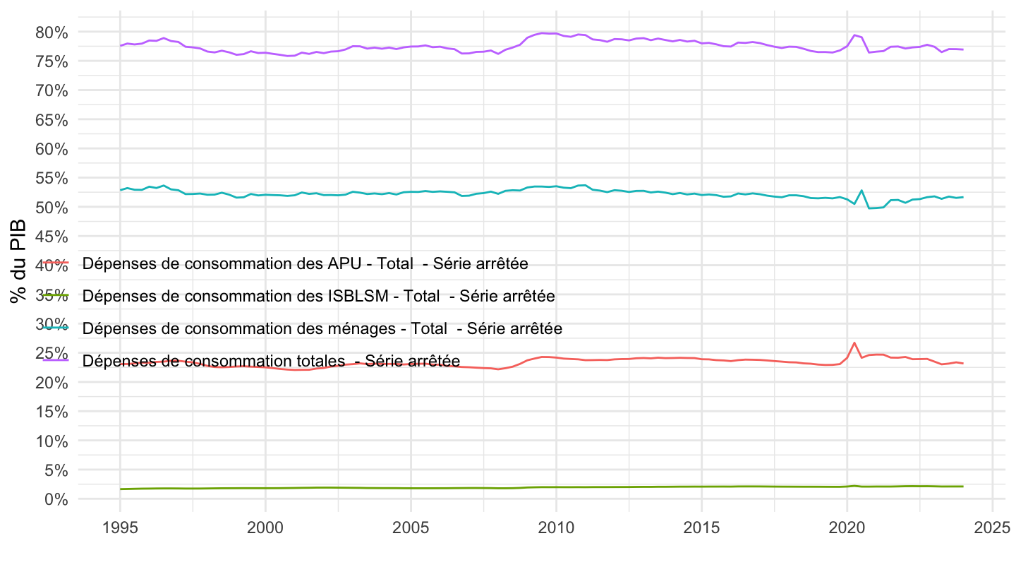
2000-
Code
`CNT-2014-PIB-EQB-RF` %>%
  filter(FREQ == "T",
         VALORISATION == "V",
         OPERATION %in% c("P4", "P3", "PIB")) %>%
  quarter_to_date %>%
  group_by(date) %>%
  mutate(OBS_VALUE = OBS_VALUE/OBS_VALUE[OPERATION == "PIB"]) %>%
  filter(OPERATION != "PIB") %>%
  mutate(TITLE_FR = gsub("- Valeur aux prix courants - Série CVS-CJO", "", TITLE_FR)) %>%
  filter(date >= as.Date("2000-01-01")) %>%
  ggplot() + ylab("% du PIB") + xlab("") + theme_minimal() +
  geom_line(aes(x = date, y = OBS_VALUE, color = TITLE_FR)) +

  scale_x_date(breaks = seq(1920, 2100, 5) %>% paste0("-01-01") %>% as.Date,
               labels = date_format("%Y")) +
  theme(legend.position = c(0.25, 0.4),
        legend.title = element_blank()) +
  scale_y_continuous(breaks = 0.01*seq(0, 300, 5),
                     labels = percent_format(accuracy = 1))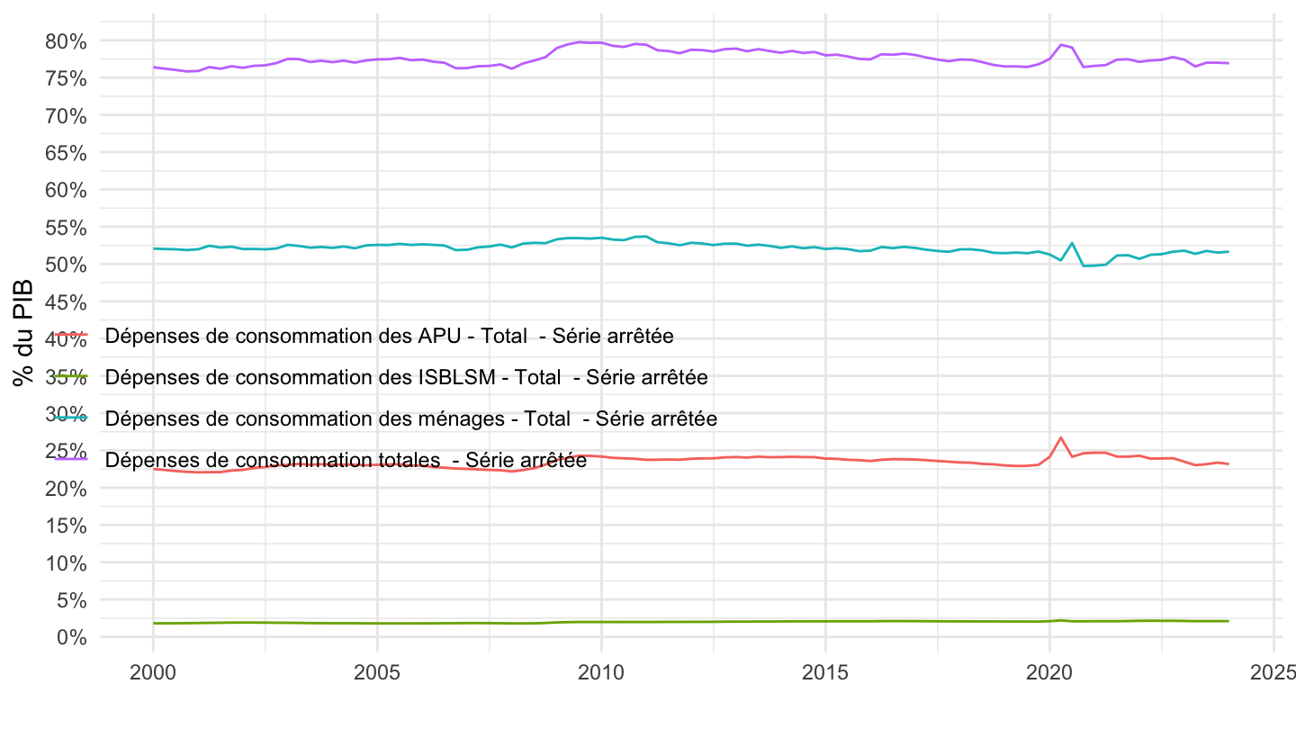
Consommation P3: individualisable P31 vs. collective P32
All
Code
`CNT-2014-PIB-EQB-RF` %>%
  filter(FREQ == "T",
         VALORISATION == "V",
         OPERATION %in% c("P31", "P32", "PIB")) %>%
  quarter_to_date %>%
  group_by(date) %>%
  mutate(OBS_VALUE = OBS_VALUE/OBS_VALUE[OPERATION == "PIB"]) %>%
  filter(OPERATION != "PIB") %>%
  mutate(TITLE_FR = gsub("- Valeur aux prix courants - Série CVS-CJO", "", TITLE_FR)) %>%
  ggplot() + ylab("% du PIB") + xlab("") + theme_minimal() +
  geom_line(aes(x = date, y = OBS_VALUE, color = TITLE_FR)) +

  scale_x_date(breaks = seq(1920, 2100, 5) %>% paste0("-01-01") %>% as.Date,
               labels = date_format("%Y")) +
  theme(legend.position = c(0.3, 0.85),
        legend.title = element_blank()) +
  scale_y_continuous(breaks = 0.01*seq(0, 300, 1),
                     labels = percent_format(accuracy = 1))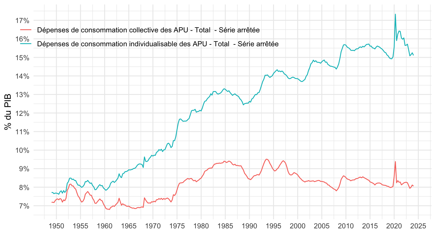
1980-
Code
`CNT-2014-PIB-EQB-RF` %>%
  filter(FREQ == "T",
         VALORISATION == "V",
         OPERATION %in% c("P31", "P32", "PIB")) %>%
  quarter_to_date %>%
  group_by(date) %>%
  mutate(OBS_VALUE = OBS_VALUE/OBS_VALUE[OPERATION == "PIB"]) %>%
  filter(OPERATION != "PIB") %>%
  mutate(TITLE_FR = gsub("- Valeur aux prix courants - Série CVS-CJO", "", TITLE_FR)) %>%
  filter(date >= as.Date("1980-01-01")) %>%
  ggplot() + ylab("% du PIB") + xlab("") + theme_minimal() +
  geom_line(aes(x = date, y = OBS_VALUE, color = TITLE_FR)) +

  scale_x_date(breaks = seq(1920, 2100, 5) %>% paste0("-01-01") %>% as.Date,
               labels = date_format("%Y")) +
  theme(legend.position = c(0.3, 0.85),
        legend.title = element_blank()) +
  scale_y_continuous(breaks = 0.01*seq(0, 300, 1),
                     labels = percent_format(accuracy = 1))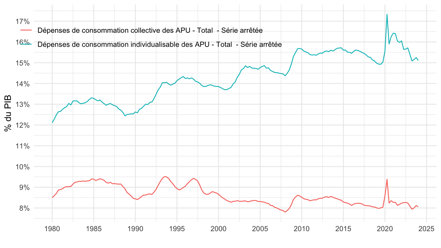
1995-
Code
`CNT-2014-PIB-EQB-RF` %>%
  filter(FREQ == "T",
         VALORISATION == "V",
         OPERATION %in% c("P31", "P32", "PIB")) %>%
  quarter_to_date %>%
  group_by(date) %>%
  mutate(OBS_VALUE = OBS_VALUE/OBS_VALUE[OPERATION == "PIB"]) %>%
  filter(OPERATION != "PIB") %>%
  mutate(TITLE_FR = gsub("- Valeur aux prix courants - Série CVS-CJO", "", TITLE_FR)) %>%
  filter(date >= as.Date("1995-01-01")) %>%
  ggplot() + ylab("% du PIB") + xlab("") + theme_minimal() +
  geom_line(aes(x = date, y = OBS_VALUE, color = TITLE_FR)) +

  scale_x_date(breaks = seq(1920, 2100, 5) %>% paste0("-01-01") %>% as.Date,
               labels = date_format("%Y")) +
  theme(legend.position = c(0.3, 0.85),
        legend.title = element_blank()) +
  scale_y_continuous(breaks = 0.01*seq(0, 300, 1),
                     labels = percent_format(accuracy = 1))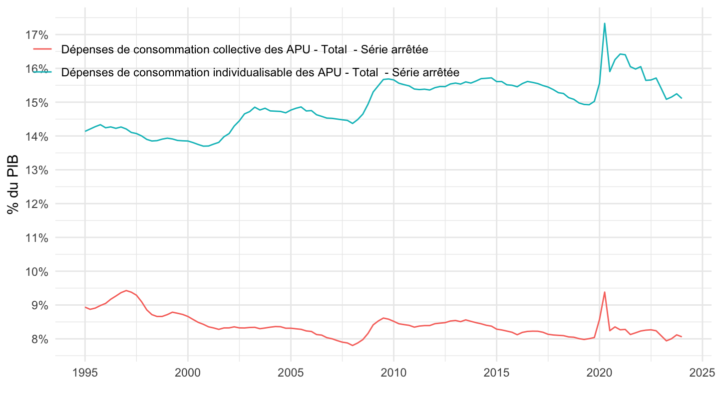
Exports, Imports
All
Code
`CNT-2014-PIB-EQB-RF` %>%
  filter(FREQ == "T",
         VALORISATION == "V",
         OPERATION %in% c("P6", "P7", "PIB")) %>%
  quarter_to_date %>%
  group_by(date) %>%
  mutate(OBS_VALUE = OBS_VALUE/OBS_VALUE[OPERATION == "PIB"]) %>%
  filter(OPERATION != "PIB") %>%
  mutate(TITLE_FR = gsub("- Valeur aux prix courants - Série CVS-CJO", "", TITLE_FR)) %>%
  ggplot() + ylab("% du PIB") + xlab("") + theme_minimal() +
  geom_line(aes(x = date, y = OBS_VALUE, color = TITLE_FR)) +

  scale_x_date(breaks = seq(1920, 2100, 5) %>% paste0("-01-01") %>% as.Date,
               labels = date_format("%Y")) +
  theme(legend.position = c(0.3, 0.85),
        legend.title = element_blank()) +
  scale_y_continuous(breaks = 0.01*seq(0, 300, 2),
                     labels = percent_format(accuracy = 1))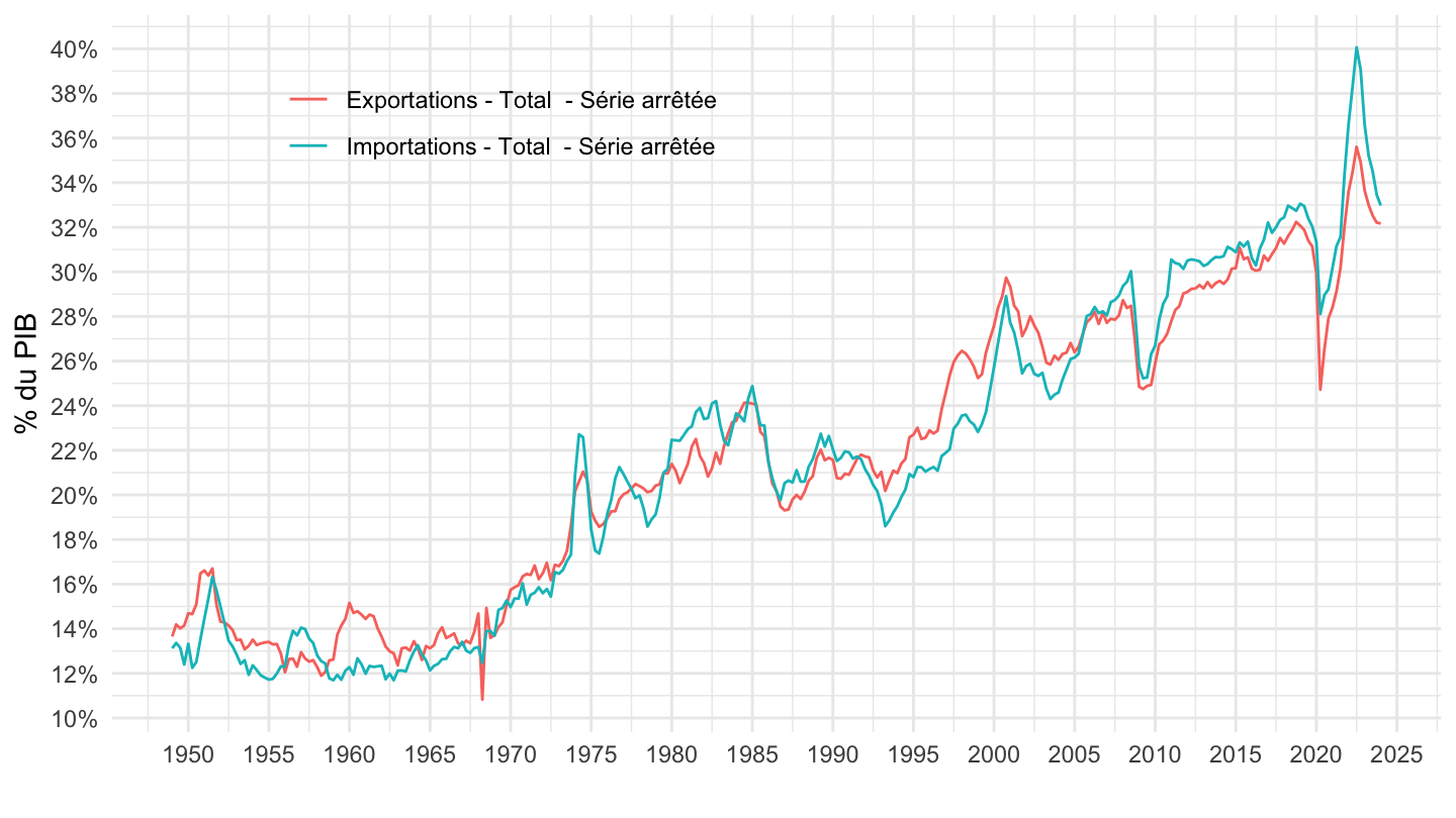
1980-
Code
`CNT-2014-PIB-EQB-RF` %>%
  filter(FREQ == "T",
         VALORISATION == "V",
         OPERATION %in% c("P6", "P7", "PIB")) %>%
  quarter_to_date %>%
  group_by(date) %>%
  mutate(OBS_VALUE = OBS_VALUE/OBS_VALUE[OPERATION == "PIB"]) %>%
  filter(OPERATION != "PIB") %>%
  mutate(TITLE_FR = gsub("- Valeur aux prix courants - Série CVS-CJO", "", TITLE_FR)) %>%
  filter(date >= as.Date("1980-01-01")) %>%
  ggplot() + ylab("% du PIB") + xlab("") + theme_minimal() +
  geom_line(aes(x = date, y = OBS_VALUE, color = TITLE_FR)) +

  scale_x_date(breaks = seq(1920, 2100, 5) %>% paste0("-01-01") %>% as.Date,
               labels = date_format("%Y")) +
  theme(legend.position = c(0.3, 0.85),
        legend.title = element_blank()) +
  scale_y_continuous(breaks = 0.01*seq(0, 300, 2),
                     labels = percent_format(accuracy = 1))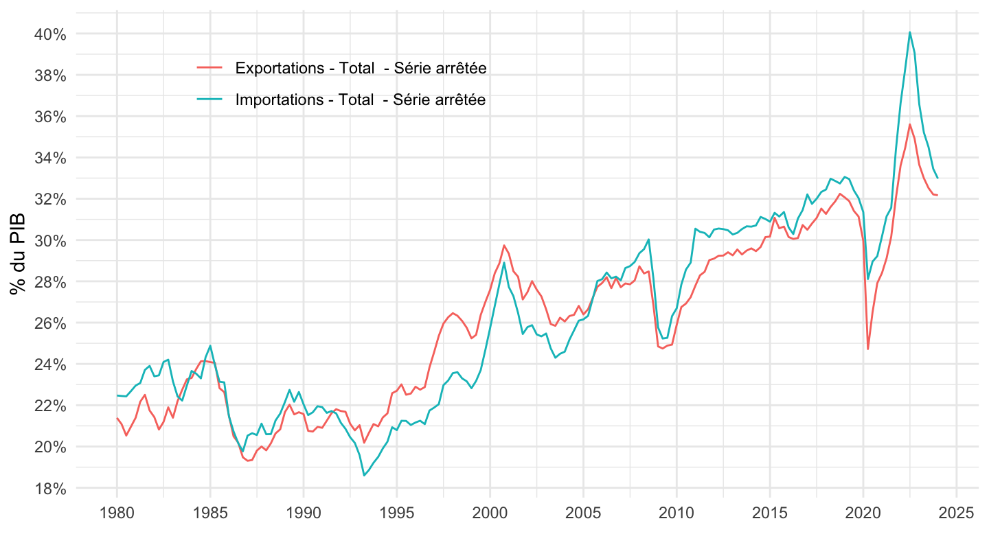
1995-
Code
`CNT-2014-PIB-EQB-RF` %>%
  filter(FREQ == "T",
         VALORISATION == "V",
         OPERATION %in% c("P6", "P7", "PIB")) %>%
  quarter_to_date %>%
  group_by(date) %>%
  mutate(OBS_VALUE = OBS_VALUE/OBS_VALUE[OPERATION == "PIB"]) %>%
  filter(OPERATION != "PIB") %>%
  mutate(TITLE_FR = gsub("- Valeur aux prix courants - Série CVS-CJO", "", TITLE_FR)) %>%
  filter(date >= as.Date("1995-01-01")) %>%
  ggplot() + ylab("% du PIB") + xlab("") + theme_minimal() +
  geom_line(aes(x = date, y = OBS_VALUE, color = TITLE_FR)) +

  scale_x_date(breaks = seq(1920, 2100, 5) %>% paste0("-01-01") %>% as.Date,
               labels = date_format("%Y")) +
  theme(legend.position = c(0.3, 0.85),
        legend.title = element_blank()) +
  scale_y_continuous(breaks = 0.01*seq(0, 300, 2),
                     labels = percent_format(accuracy = 1))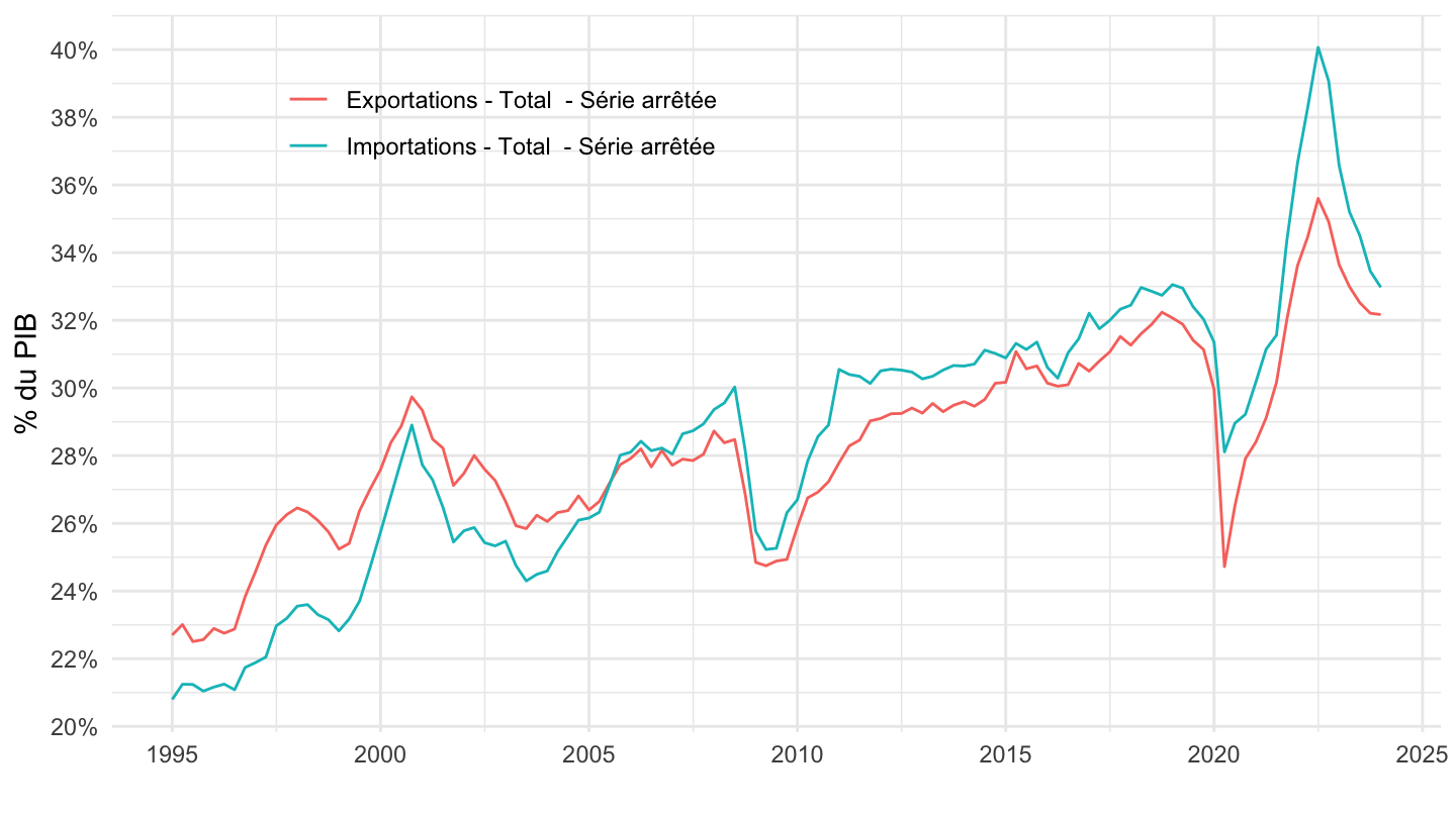
Solde Extérieur
All
Code
`CNT-2014-PIB-EQB-RF` %>%
  filter(FREQ == "T",
         VALORISATION == "V",
         OPERATION %in% c("SOLDE", "PIB")) %>%
  quarter_to_date %>%
  group_by(date) %>%
  mutate(OBS_VALUE = OBS_VALUE/OBS_VALUE[OPERATION == "PIB"]) %>%
  filter(OPERATION != "PIB") %>%
  mutate(TITLE_FR = gsub("- Valeur aux prix courants - Série CVS-CJO", "", TITLE_FR)) %>%
  na.omit %>%
  ggplot() + ylab("% du PIB") + xlab("") + theme_minimal() +
  geom_line(aes(x = date, y = OBS_VALUE, color = TITLE_FR)) +

  scale_x_date(breaks = seq(1920, 2100, 5) %>% paste0("-01-01") %>% as.Date,
               labels = date_format("%Y")) +
  theme(legend.position = c(0.3, 0.85),
        legend.title = element_blank()) +
  scale_y_continuous(breaks = 0.01*seq(-100, 300, 1),
                     labels = percent_format(accuracy = 1))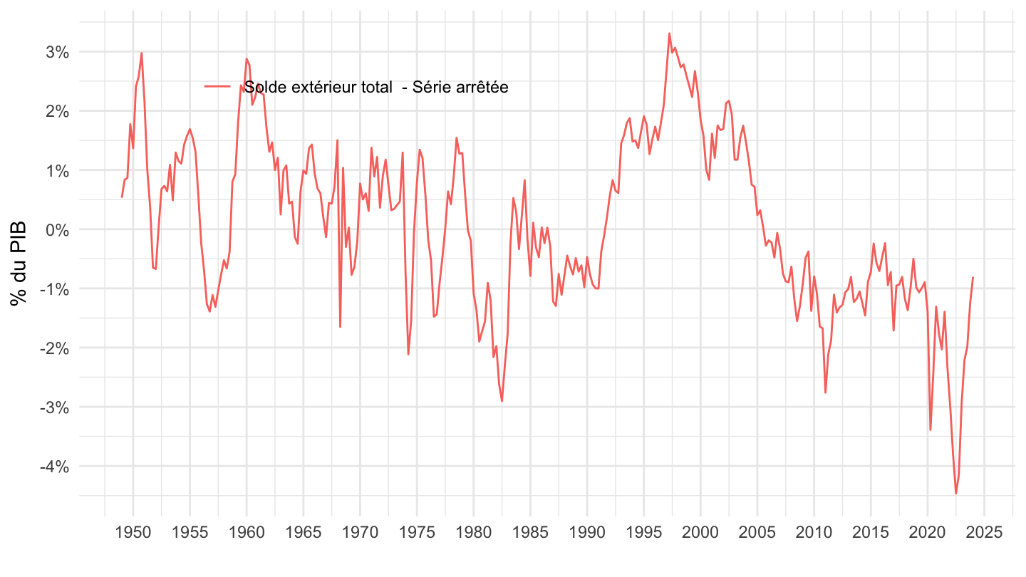
1980-
Code
`CNT-2014-PIB-EQB-RF` %>%
  filter(FREQ == "T",
         VALORISATION == "V",
         OPERATION %in% c("SOLDE", "PIB")) %>%
  quarter_to_date %>%
  group_by(date) %>%
  mutate(OBS_VALUE = OBS_VALUE/OBS_VALUE[OPERATION == "PIB"]) %>%
  filter(OPERATION != "PIB") %>%
  mutate(TITLE_FR = gsub("- Valeur aux prix courants - Série CVS-CJO", "", TITLE_FR)) %>%
  na.omit %>%
  filter(date >= as.Date("1980-01-01")) %>%
  ggplot() + ylab("% du PIB") + xlab("") + theme_minimal() +
  geom_line(aes(x = date, y = OBS_VALUE, color = TITLE_FR)) +

  scale_x_date(breaks = seq(1920, 2100, 5) %>% paste0("-01-01") %>% as.Date,
               labels = date_format("%Y")) +
  theme(legend.position = c(0.3, 0.85),
        legend.title = element_blank()) +
  scale_y_continuous(breaks = 0.01*seq(-100, 300, 1),
                     labels = percent_format(accuracy = 1))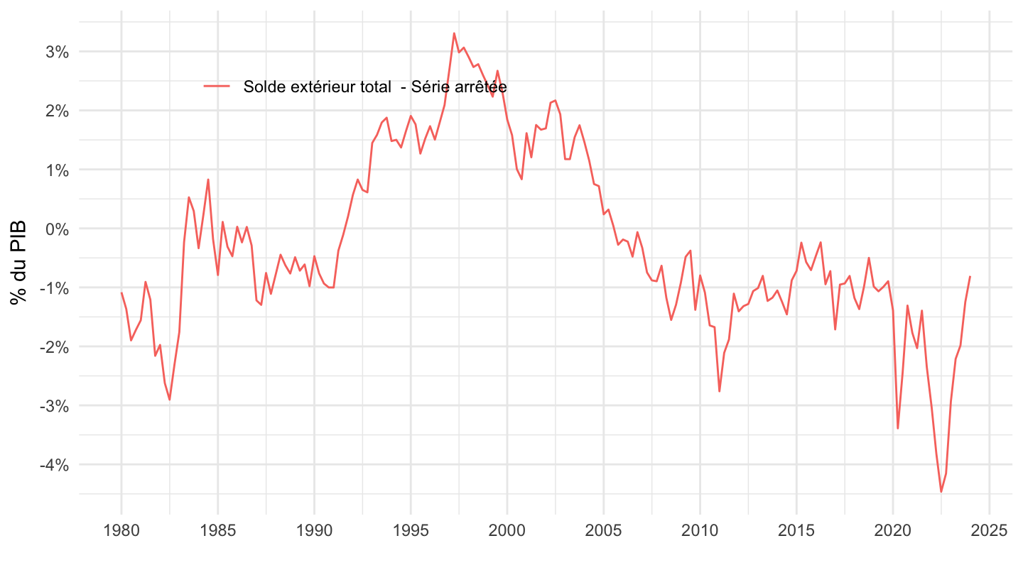
1995-
Code
`CNT-2014-PIB-EQB-RF` %>%
  filter(FREQ == "T",
         VALORISATION == "V",
         OPERATION %in% c("SOLDE", "PIB")) %>%
  quarter_to_date %>%
  group_by(date) %>%
  mutate(OBS_VALUE = OBS_VALUE/OBS_VALUE[OPERATION == "PIB"]) %>%
  filter(OPERATION != "PIB") %>%
  mutate(TITLE_FR = gsub("- Valeur aux prix courants - Série CVS-CJO", "", TITLE_FR)) %>%
  na.omit %>%
  filter(date >= as.Date("1995-01-01")) %>%
  ggplot() + ylab("% du PIB") + xlab("") + theme_minimal() +
  geom_line(aes(x = date, y = OBS_VALUE, color = TITLE_FR)) +

  scale_x_date(breaks = seq(1920, 2100, 5) %>% paste0("-01-01") %>% as.Date,
               labels = date_format("%Y")) +
  theme(legend.position = c(0.3, 0.85),
        legend.title = element_blank()) +
  scale_y_continuous(breaks = 0.01*seq(-100, 300, 1),
                     labels = percent_format(accuracy = 1))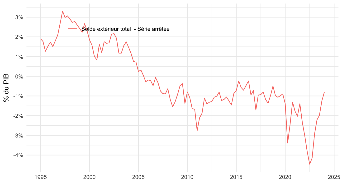
Investissement
All
Code
`CNT-2014-PIB-EQB-RF` %>%
  filter(FREQ == "T",
         VALORISATION == "V",
         OPERATION %in% c("P51", "P51B", "P51G", "P51M", "P51P", "P51S", "PIB")) %>%
  quarter_to_date %>%
  group_by(date) %>%
  mutate(OBS_VALUE = OBS_VALUE/OBS_VALUE[OPERATION == "PIB"]) %>%
  filter(OPERATION != "PIB") %>%
  mutate(TITLE_FR = gsub("- Valeur aux prix courants - Série CVS-CJO", "", TITLE_FR)) %>%
  ggplot() + ylab("% du PIB") + xlab("") + theme_minimal() +
  geom_line(aes(x = date, y = OBS_VALUE, color = paste(OPERATION, "-", TITLE_FR))) +
  #
  scale_x_date(breaks = seq(1920, 2100, 5) %>% paste0("-01-01") %>% as.Date,
               labels = date_format("%Y")) +
  theme(legend.position = c(0.3, 0.78),
        legend.title = element_blank()) +
  scale_y_continuous(breaks = 0.01*seq(0, 300, 2),
                     labels = percent_format(accuracy = 1))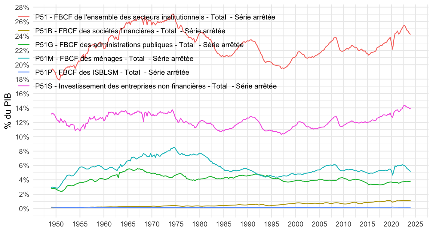
1980-
Code
`CNT-2014-PIB-EQB-RF` %>%
  filter(FREQ == "T",
         VALORISATION == "V",
         OPERATION %in% c("P51", "P51B", "P51G", "P51M", "P51P", "P51S", "PIB")) %>%
  quarter_to_date %>%
  group_by(date) %>%
  mutate(OBS_VALUE = OBS_VALUE/OBS_VALUE[OPERATION == "PIB"]) %>%
  filter(OPERATION != "PIB") %>%
  mutate(TITLE_FR = gsub("- Valeur aux prix courants - Série CVS-CJO", "", TITLE_FR)) %>%
  filter(date >= as.Date("1980-01-01")) %>%
  ggplot() + ylab("% du PIB") + xlab("") + theme_minimal() +
  geom_line(aes(x = date, y = OBS_VALUE, color = TITLE_FR)) +
  #
  scale_x_date(breaks = seq(1920, 2100, 5) %>% paste0("-01-01") %>% as.Date,
               labels = date_format("%Y")) +
  theme(legend.position = c(0.3, 0.8),
        legend.title = element_blank()) +
  scale_y_continuous(breaks = 0.01*seq(0, 300, 2),
                     labels = percent_format(accuracy = 1))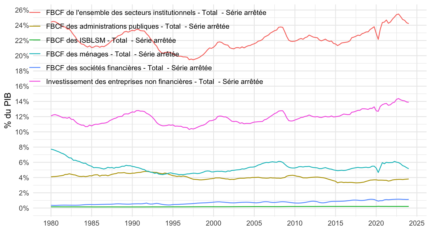
1995-
Code
`CNT-2014-PIB-EQB-RF` %>%
  filter(FREQ == "T",
         VALORISATION == "V",
         OPERATION %in% c("P51", "P51B", "P51G", "P51M", "P51P", "P51S", "PIB")) %>%
  quarter_to_date %>%
  group_by(date) %>%
  mutate(OBS_VALUE = OBS_VALUE/OBS_VALUE[OPERATION == "PIB"]) %>%
  filter(OPERATION != "PIB") %>%
  mutate(TITLE_FR = gsub("- Valeur aux prix courants - Série CVS-CJO", "", TITLE_FR)) %>%
  filter(date >= as.Date("1995-01-01")) %>%
  ggplot() + ylab("% du PIB") + xlab("") + theme_minimal() +
  geom_line(aes(x = date, y = OBS_VALUE, color = TITLE_FR)) +
  #
  scale_x_date(breaks = seq(1920, 2100, 5) %>% paste0("-01-01") %>% as.Date,
               labels = date_format("%Y")) +
  theme(legend.position = c(0.3, 0.8),
        legend.title = element_blank()) +
  scale_y_continuous(breaks = 0.01*seq(0, 300, 2),
                     labels = percent_format(accuracy = 1))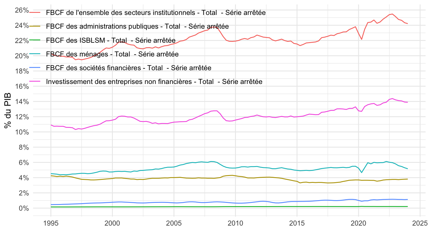
GDP Updates
gdp_quarterly2
Code
gdp_quarterly <- `CNT-2014-PIB-EQB-RF` %>%
  filter(OPERATION == "PIB",
         FREQ == "T",
         VALORISATION == "V") %>%
  quarter_to_date %>%
  arrange(date) %>%
  mutate(date = date + months(3) - days(1)) %>%
  select(date, gdp = OBS_VALUE) %>%
  mutate(gdp = gdp/1000)

save(gdp_quarterly, file = "gdp_quarterly2.RData")

gdp_quarterly %>%
  tail(5) %>%
print_table_conditional()| date | gdp |
|---|---|
| 2023-03-31 | 685.694 |
| 2023-06-30 | 701.202 |
| 2023-09-30 | 706.297 |
| 2023-12-31 | 712.478 |
| 2024-03-31 | 719.086 |
gdp_quarterly3
Code
gdp_quarterly <- `CNT-2014-PIB-EQB-RF` %>%
  filter(OPERATION == "PIB",
         FREQ == "T",
         VALORISATION == "V") %>%
  quarter_to_date %>%
  arrange(date) %>%
  select(date, gdp = OBS_VALUE) %>%
  mutate(gdp = gdp/1000)

save(gdp_quarterly, file = "gdp_quarterly3.RData")

gdp_quarterly %>%
  tail(5) %>%
print_table_conditional()| date | gdp |
|---|---|
| 2023-01-01 | 685.694 |
| 2023-04-01 | 701.202 |
| 2023-07-01 | 706.297 |
| 2023-10-01 | 712.478 |
| 2024-01-01 | 719.086 |
gdp_quarterly4: IDBANK 010565707
Code
gdp_quarterly <- `CNT-2014-PIB-EQB-RF` %>%
  filter(OPERATION == "PIB",
         FREQ == "T",
         VALORISATION == "V") %>%
  quarter_to_date %>%
  arrange(date) %>%
  select(date, gdp = OBS_VALUE)

save(gdp_quarterly, file = "gdp_quarterly4.RData")

gdp_quarterly %>%
  tail(5) %>%
print_table_conditional()| date | gdp |
|---|---|
| 2023-01-01 | 685694 |
| 2023-04-01 | 701202 |
| 2023-07-01 | 706297 |
| 2023-10-01 | 712478 |
| 2024-01-01 | 719086 |
Depuis le Covid-19
PIB valeur
Code
`CNT-2014-PIB-EQB-RF` %>%
  filter(OPERATION %in% c("PIB", "P3", "P31", "P32", "P4"),
         FREQ == "T",
         VALORISATION == "V",
         NATURE == "VALEUR_ABSOLUE",
         `SECT-INST` == "SO") %>%

  quarter_to_date %>%
  filter(date >= as.Date("2019-10-01")) %>%
  select_if(~ n_distinct(.) > 1) %>%
  arrange(date) %>%
  group_by(OPERATION) %>%
  mutate(OBS_VALUE = 100*OBS_VALUE/OBS_VALUE[date == as.Date("2019-10-01")]) %>%
  ggplot + geom_line(aes(x = date, y = OBS_VALUE, color = Operation)) +
  xlab("") + ylab("") +  theme_minimal() +
  scale_x_date(breaks = seq.Date(from = as.Date("2019-10-01"), to = as.Date("2023-10-01"), by = "quarter"),
               labels = date_format("%b %y")) +
  scale_y_log10(breaks = seq(0, 120, 5)) +
  theme(legend.position = c(0.7, 0.2),
        legend.title = element_blank())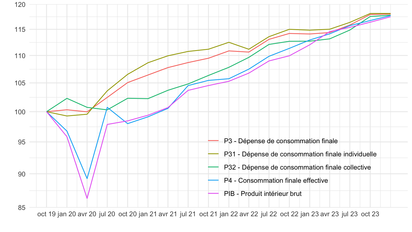
PIB volume
2019-Q4
Code
`CNT-2014-PIB-EQB-RF` %>%
  filter(OPERATION %in% c("PIB", "P3", "P31", "P32", "P4"),
         FREQ == "T",
         VALORISATION == "L",
         NATURE == "VALEUR_ABSOLUE",
         `SECT-INST` == "SO") %>%

  quarter_to_date %>%
  filter(date >= as.Date("2019-10-01")) %>%
  select_if(~ n_distinct(.) > 1) %>%
  arrange(date) %>%
  group_by(OPERATION) %>%
  mutate(OBS_VALUE = 100*OBS_VALUE/OBS_VALUE[date == as.Date("2019-10-01")]) %>%
  ggplot + geom_line(aes(x = date, y = OBS_VALUE, color = Operation)) +
  xlab("") + ylab("") +  theme_minimal() +
  scale_x_date(breaks = seq.Date(from = as.Date("2019-10-01"), to = as.Date("2023-10-01"), by = "quarter"),
               labels = date_format("%b %y")) +
  scale_y_log10(breaks = seq(0, 120, 5)) +
  theme(legend.position = c(0.7, 0.2),
        legend.title = element_blank())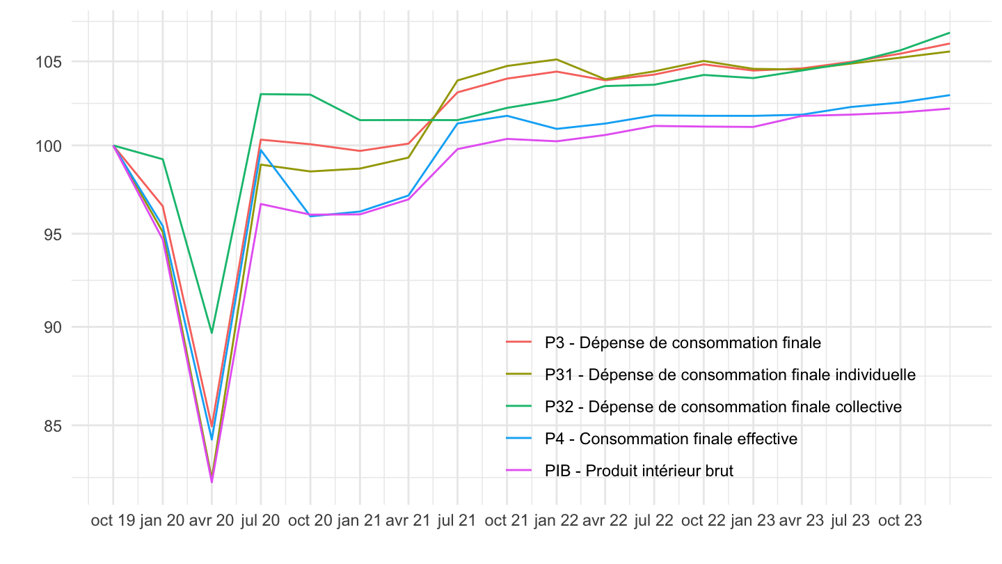
Demande, Demande hors stocks
Code
`CNT-2014-PIB-EQB-RF` %>%
  filter(OPERATION %in% c("PIB", "DINTF", "DINTFHS"),
         FREQ == "T",
         VALORISATION == "L",
         NATURE == "VALEUR_ABSOLUE",
         `SECT-INST` == "SO") %>%

  quarter_to_date %>%
  filter(date >= as.Date("2019-10-01")) %>%
  select_if(~ n_distinct(.) > 1) %>%
  arrange(date) %>%
  group_by(OPERATION) %>%
  mutate(OBS_VALUE = 100*OBS_VALUE/OBS_VALUE[date == as.Date("2019-10-01")]) %>%
  ggplot + geom_line(aes(x = date, y = OBS_VALUE, color = Operation)) +
  xlab("") + ylab("") +  theme_minimal() +
  scale_x_date(breaks = seq.Date(from = as.Date("2019-10-01"), to = as.Date("2023-10-01"), by = "quarter"),
               labels = date_format("%b %y")) +
  scale_y_log10(breaks = seq(0, 120, 5)) +
  theme(legend.position = c(0.7, 0.2),
        legend.title = element_blank())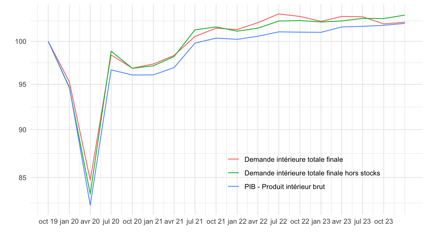
2017-Q2 -
PIB valeur
Code
`CNT-2014-PIB-EQB-RF` %>%
  filter(OPERATION %in% c("PIB", "P3", "P31", "P32", "P4"),
         FREQ == "T",
         VALORISATION == "V",
         NATURE == "VALEUR_ABSOLUE",
         `SECT-INST` == "SO") %>%

  quarter_to_date %>%
  filter(date >= as.Date("2017-04-01")) %>%
  select_if(~ n_distinct(.) > 1) %>%
  arrange(date) %>%
  group_by(OPERATION) %>%
  mutate(OBS_VALUE = 100*OBS_VALUE/OBS_VALUE[date == as.Date("2017-04-01")]) %>%
  ggplot + geom_line(aes(x = date, y = OBS_VALUE, color = Operation)) +
  xlab("") + ylab("") +  theme_minimal() +
  scale_x_date(breaks = seq.Date(from = as.Date("2017-04-01"), to = as.Date("2023-10-01"), by = "6 months"),
               labels = date_format("%b %y")) +
  scale_y_log10(breaks = c(seq(0, 120, 5), 106, 107, 111, 112, 113)) +
  theme(legend.position = c(0.3, 0.2),
        legend.title = element_blank())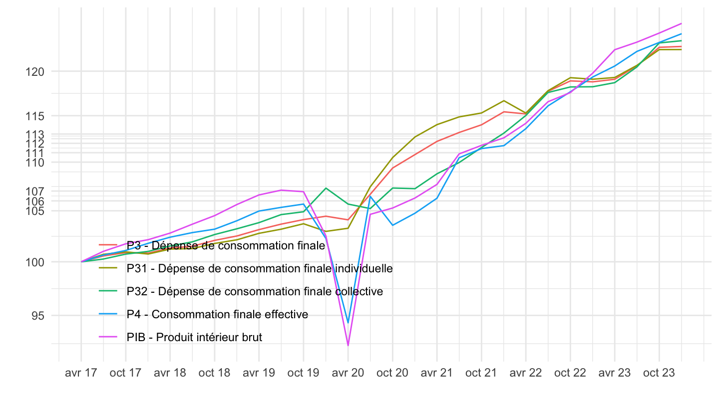
PIB volume
Code
`CNT-2014-PIB-EQB-RF` %>%
  filter(OPERATION %in% c("PIB", "P3", "P31", "P32", "P4"),
         FREQ == "T",
         VALORISATION == "L",
         NATURE == "VALEUR_ABSOLUE",
         `SECT-INST` == "SO") %>%

  quarter_to_date %>%
  filter(date >= as.Date("2017-04-01")) %>%
  select_if(~ n_distinct(.) > 1) %>%
  arrange(date) %>%
  group_by(OPERATION) %>%
  mutate(OBS_VALUE = 100*OBS_VALUE/OBS_VALUE[date == as.Date("2017-04-01")]) %>%
  ggplot + geom_line(aes(x = date, y = OBS_VALUE, color = Operation)) +
  xlab("") + ylab("") +  theme_minimal() +
  scale_x_date(breaks = seq.Date(from = as.Date("2017-04-01"), to = as.Date("2023-10-01"), by = "6 months"),
               labels = date_format("%b %y")) +
  scale_y_log10(breaks = c(seq(0, 120, 5), 106, 107)) +
  theme(legend.position = c(0.3, 0.2),
        legend.title = element_blank())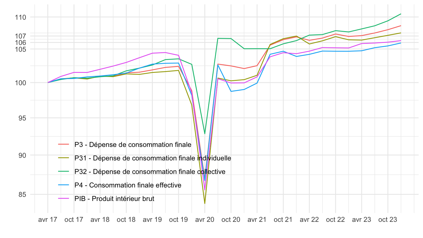
Demande, Demande hors stocks
Code
`CNT-2014-PIB-EQB-RF` %>%
  filter(OPERATION %in% c("PIB", "DINTF", "DINTFHS"),
         FREQ == "T",
         VALORISATION == "L",
         NATURE == "VALEUR_ABSOLUE",
         `SECT-INST` == "SO") %>%

  quarter_to_date %>%
  filter(date >= as.Date("2017-04-01")) %>%
  select_if(~ n_distinct(.) > 1) %>%
  arrange(date) %>%
  group_by(OPERATION) %>%
  mutate(OBS_VALUE = 100*OBS_VALUE/OBS_VALUE[date == as.Date("2017-04-01")]) %>%
  ggplot + geom_line(aes(x = date, y = OBS_VALUE, color = Operation)) +
  xlab("") + ylab("") +  theme_minimal() +
  scale_x_date(breaks = seq.Date(from = as.Date("2017-04-01"), to = as.Date("2023-10-01"), by = "6 months"),
               labels = date_format("%b %y")) +
  scale_y_log10(breaks = seq(0, 120, 5)) +
  theme(legend.position = c(0.3, 0.2),
        legend.title = element_blank())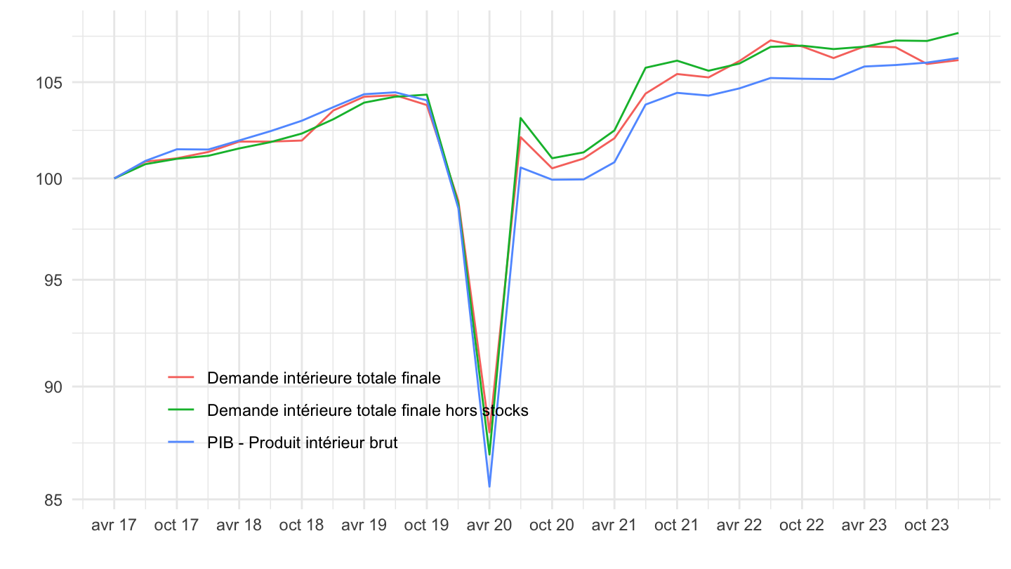
2011-Q1
PIB valeur
Code
`CNT-2014-PIB-EQB-RF` %>%
  filter(OPERATION %in% c("PIB", "P3", "P31", "P32", "P4"),
         FREQ == "T",
         VALORISATION == "V",
         NATURE == "VALEUR_ABSOLUE",
         `SECT-INST` == "SO") %>%

  quarter_to_date %>%
  filter(date >= as.Date("2011-01-01")) %>%
  select_if(~ n_distinct(.) > 1) %>%
  arrange(date) %>%
  group_by(OPERATION) %>%
  mutate(OBS_VALUE = 100*OBS_VALUE/OBS_VALUE[date == as.Date("2011-01-01")]) %>%
  ggplot + geom_line(aes(x = date, y = OBS_VALUE, color = Operation)) +
  xlab("") + ylab("") +  theme_minimal() +
  scale_x_date(breaks = "1 year",
               labels = date_format("%Y")) +
  scale_y_log10(breaks = c(seq(0, 170, 5), 106, 107, 111, 112, 113)) +
  theme(legend.position = c(0.3, 0.8),
        legend.title = element_blank())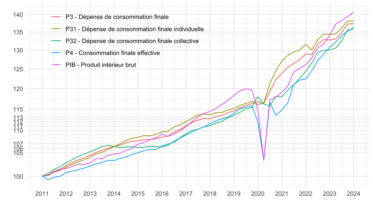
PIB volume
Code
`CNT-2014-PIB-EQB-RF` %>%
  filter(OPERATION %in% c("PIB", "P3", "P31", "P32", "P4"),
         FREQ == "T",
         VALORISATION == "L",
         NATURE == "VALEUR_ABSOLUE",
         `SECT-INST` == "SO") %>%

  quarter_to_date %>%
  filter(date >= as.Date("2010-01-01")) %>%
  select_if(~ n_distinct(.) > 1) %>%
  arrange(date) %>%
  group_by(OPERATION) %>%
  mutate(OBS_VALUE = 100*OBS_VALUE/OBS_VALUE[date == as.Date("2010-01-01")]) %>%
  ggplot + geom_line(aes(x = date, y = OBS_VALUE, color = Operation)) +
  xlab("") + ylab("") +  theme_minimal() +
  scale_x_date(breaks = "1 year",
               labels = date_format("%Y")) +
  scale_y_log10(breaks = c(seq(0, 180, 5), 106, 107)) +
  theme(legend.position = c(0.3, 0.8),
        legend.title = element_blank())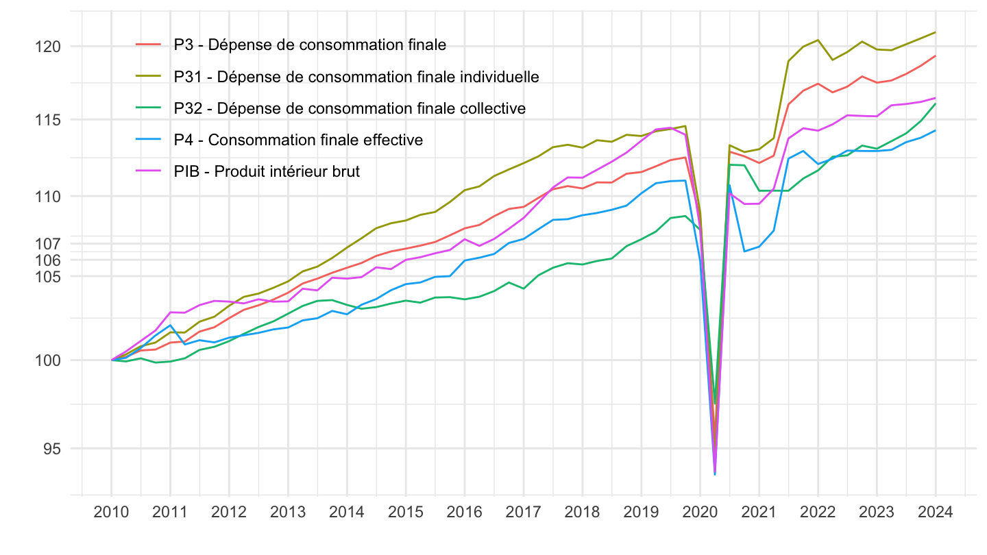
2011-14
PIB valeur
Code
`CNT-2014-PIB-EQB-RF` %>%
  filter(OPERATION %in% c("PIB", "P3", "P31", "P32", "P4"),
         FREQ == "T",
         VALORISATION == "V",
         NATURE == "VALEUR_ABSOLUE",
         `SECT-INST` == "SO") %>%

  quarter_to_date %>%
  filter(date >= as.Date("2011-01-01"),
         date <= as.Date("2014-01-01")) %>%
  select_if(~ n_distinct(.) > 1) %>%
  arrange(date) %>%
  group_by(OPERATION) %>%
  mutate(OBS_VALUE = 100*OBS_VALUE/OBS_VALUE[date == as.Date("2011-01-01")]) %>%
  ggplot + geom_line(aes(x = date, y = OBS_VALUE, color = Operation)) +
  xlab("") + ylab("") +  theme_minimal() +
  scale_x_date(breaks = "1 year",
               labels = date_format("%Y")) +
  scale_y_log10(breaks = c(seq(0, 170, 1), 106, 107, 111, 112, 113)) +
  theme(legend.position = c(0.3, 0.8),
        legend.title = element_blank())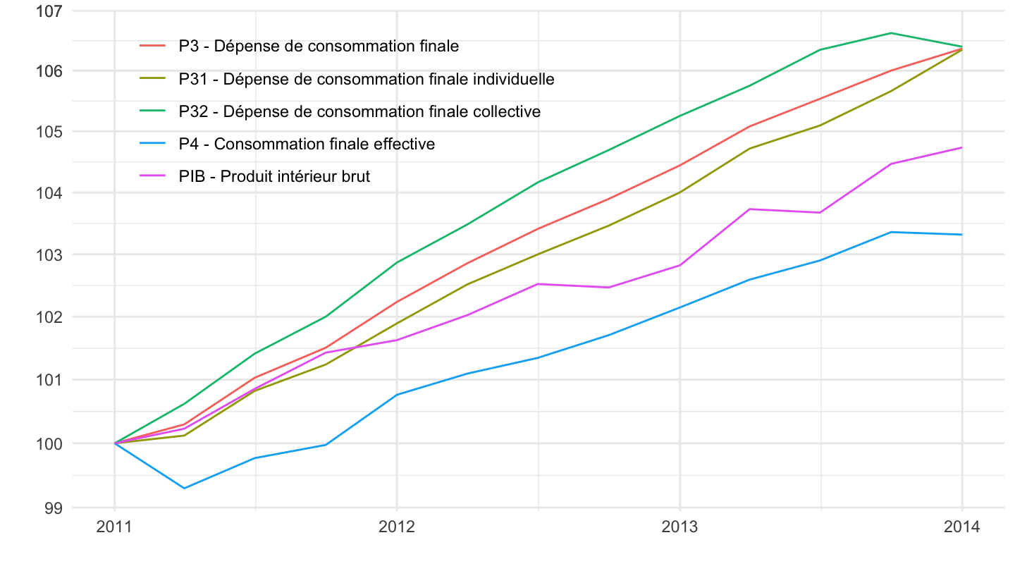
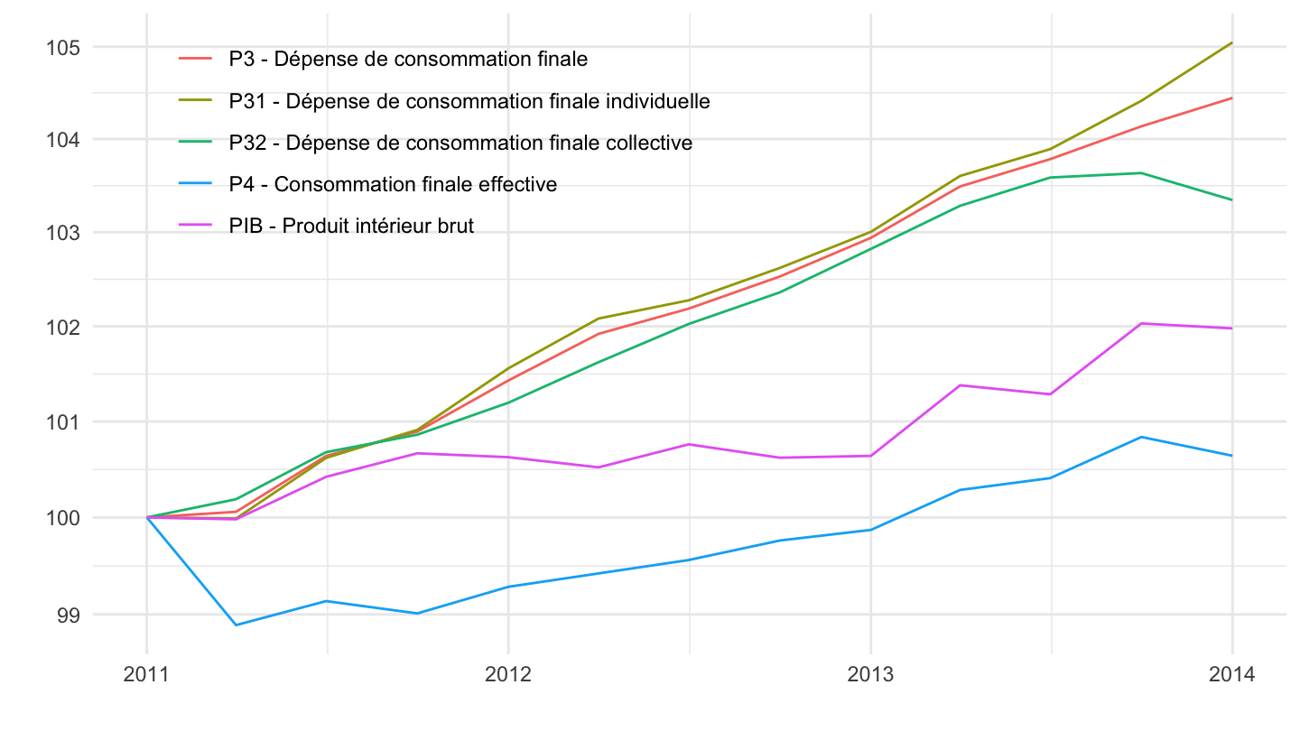
PIB volume
Code
`CNT-2014-PIB-EQB-RF` %>%
  filter(OPERATION %in% c("PIB", "P3", "P31", "P32", "P4"),
         FREQ == "T",
         VALORISATION == "L",
         NATURE == "VALEUR_ABSOLUE",
         `SECT-INST` == "SO") %>%

  quarter_to_date %>%
  filter(date >= as.Date("2011-01-01"),
         date <= as.Date("2014-01-01")) %>%
  select_if(~ n_distinct(.) > 1) %>%
  arrange(date) %>%
  group_by(OPERATION) %>%
  mutate(OBS_VALUE = 100*OBS_VALUE/OBS_VALUE[date == as.Date("2011-01-01")]) %>%
  ggplot + geom_line(aes(x = date, y = OBS_VALUE, color = Operation)) +
  xlab("") + ylab("") +  theme_minimal() +
  scale_x_date(breaks = "1 year",
               labels = date_format("%Y")) +
  scale_y_log10(breaks = c(seq(0, 180, 1), 106, 107)) +
  theme(legend.position = c(0.3, 0.8),
        legend.title = element_blank())