Consommation des ménages - CNA-2014-CONSO-MEN

Name: Consommation des ménages
Creator: François Geerolf
License: https://www.etalab.gouv.fr/licence-ouverte-open-licence/

Données - INSEE

Auteur

François Geerolf

Last observation: 2022 (N = 13)

First observation: 1949 (N = 6)

Last data update: 04 sept. 2026, 00:36

Last compile: 04 sept. 2026, 01:48

Structure

LAST_DOWNLOAD

dataset	LAST_DOWNLOAD
CNA-2014-CONSO-MEN	2026-07-23 03:40:48
CNA-2014-PIB	2026-07-04 12:44:09
IPC-PM-2015	NA

% de la consommation des ménages, postes

FON01, FON02, FON03, FON04

Code

`CNA-2014-CONSO-MEN` |>
  filter(CNA_PRODUIT %in% c("FON01", "FON02", "FON03", "FON04"),
         NATURE == "VALEUR_ABSOLUE",
         PRIX_REF == "VAL") |>
  #select_if(~ n_distinct(.) > 1) %>%
  year_to_date() |>
  left_join(conso_menages, by = "date") |>
  
  ggplot() + theme_minimal() + ylab("Consommation (% de la consommation des ménages)") + xlab("") +
  geom_line(aes(x = date, y = OBS_VALUE/(conso_menages), color = CNA_PRODUIT)) +
  theme(legend.title = element_blank(),
        legend.position = c(0.4, 0.8)) +
  scale_x_date(breaks = seq(1950, 2100, 5) |> paste0("-01-01") |> as.Date(),
               labels = date_format("%Y")) +
  
  scale_y_continuous(breaks = 0.01*seq(0, 100, 2),
                     labels = scales::percent_format(accuracy = 1))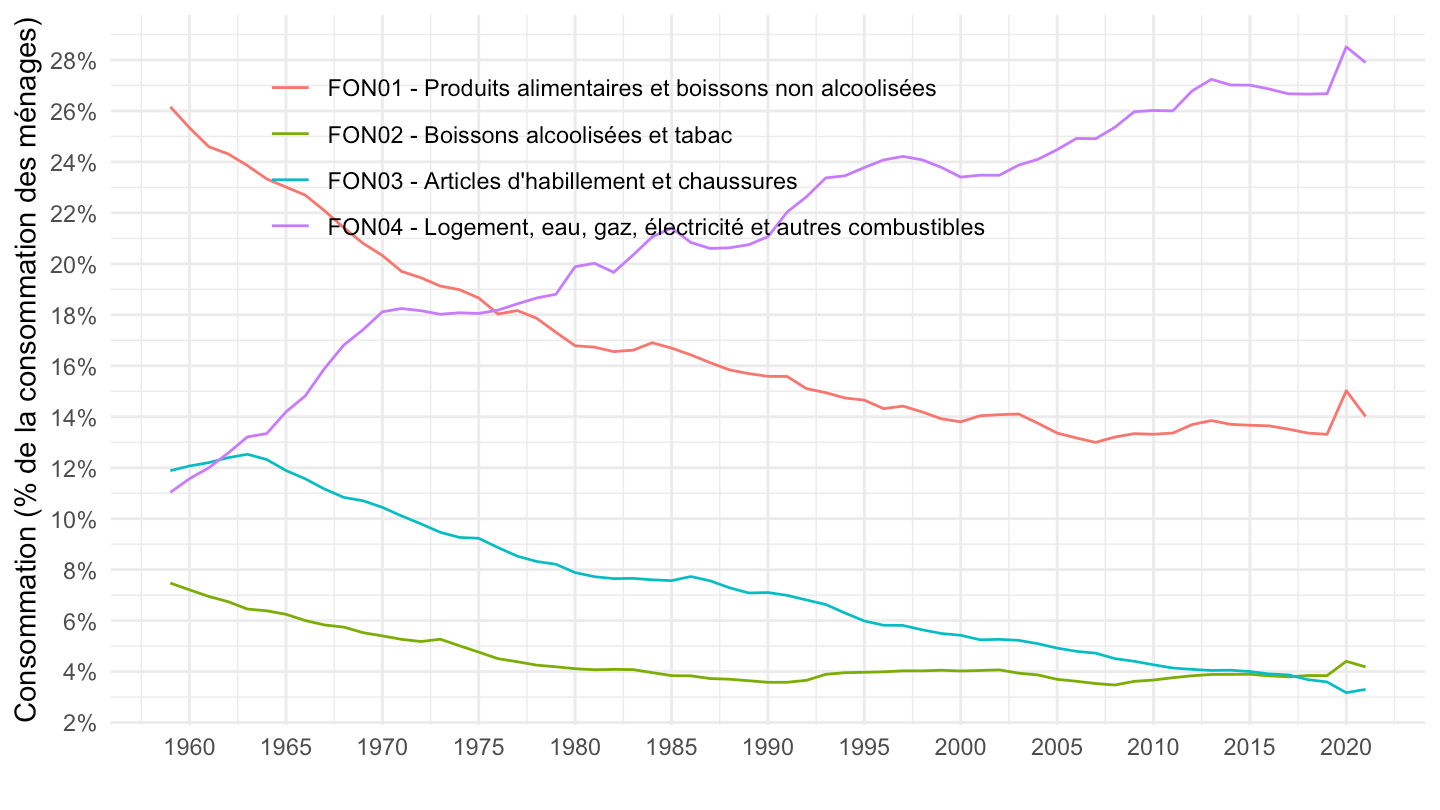

FON05, FON06, FON07, FON08

Code

`CNA-2014-CONSO-MEN` |>
  filter(CNA_PRODUIT %in% c("FON05", "FON06", "FON07", "FON08"),
         NATURE == "VALEUR_ABSOLUE",
         PRIX_REF == "VAL") |>
  #select_if(~ n_distinct(.) > 1) %>%
  year_to_date() |>
  left_join(conso_menages, by = "date") |>
  
  ggplot() + theme_minimal() + ylab("Consommation (% de la consommation des ménages)") + xlab("") +
  geom_line(aes(x = date, y = OBS_VALUE/(conso_menages), color = CNA_PRODUIT)) +
  theme(legend.title = element_blank(),
        legend.position = c(0.4, 0.8)) +
  scale_x_date(breaks = seq(1950, 2100, 5) |> paste0("-01-01") |> as.Date(),
               labels = date_format("%Y")) +
  
  scale_y_continuous(breaks = 0.01*seq(0, 100, 2),
                     labels = scales::percent_format(accuracy = 1))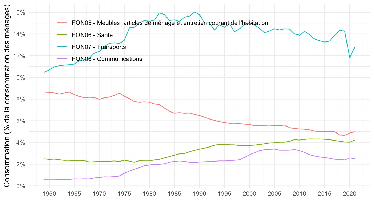

FON09, FON10, FON11, FON12

Code

`CNA-2014-CONSO-MEN` |>
  filter(CNA_PRODUIT %in% c("FON09", "FON10", "FON11", "FON12"),
         NATURE == "VALEUR_ABSOLUE",
         PRIX_REF == "VAL") |>
  #select_if(~ n_distinct(.) > 1) %>%
  year_to_date() |>
  left_join(conso_menages, by = "date") |>
  
  ggplot() + theme_minimal() + ylab("Consommation (% de la consommation des ménages)") + xlab("") +
  geom_line(aes(x = date, y = OBS_VALUE/(conso_menages), color = CNA_PRODUIT)) +
  theme(legend.title = element_blank(),
        legend.position = c(0.4, 0.8)) +
  scale_x_date(breaks = seq(1950, 2100, 5) |> paste0("-01-01") |> as.Date(),
               labels = date_format("%Y")) +
  
  scale_y_continuous(breaks = 0.01*seq(0, 100, 2),
                     labels = scales::percent_format(accuracy = 1))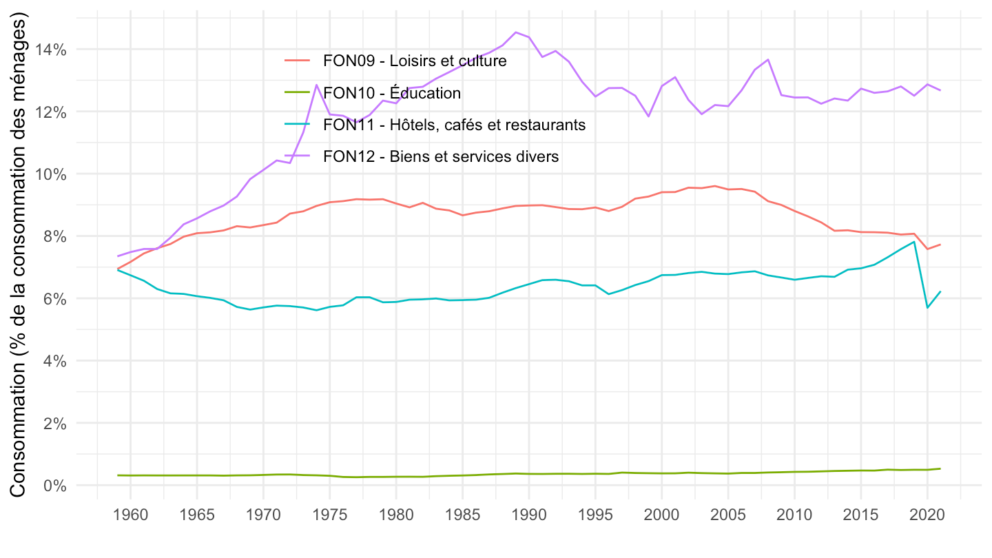

FON081, FON082, FON083

Code

`CNA-2014-CONSO-MEN` |>
  filter(CNA_PRODUIT %in% c("FON081", "FON082", "FON083", "FON08"),
         NATURE == "VALEUR_ABSOLUE",
         PRIX_REF == "VAL") |>
  #select_if(~ n_distinct(.) > 1) %>%
  year_to_date() |>
  left_join(conso_menages, by = "date") |>
  
  ggplot() + theme_minimal() + ylab("Consommation (% de la consommation des ménages)") + xlab("") +
  geom_line(aes(x = date, y = OBS_VALUE/(conso_menages), color = CNA_PRODUIT)) +
  theme(legend.title = element_blank(),
        legend.position = c(0.4, 0.8)) +
  scale_x_date(breaks = seq(1950, 2100, 5) |> paste0("-01-01") |> as.Date(),
               labels = date_format("%Y")) +
  
  scale_y_continuous(breaks = 0.01*seq(0, 100, 1),
                     labels = scales::percent_format(accuracy = 1))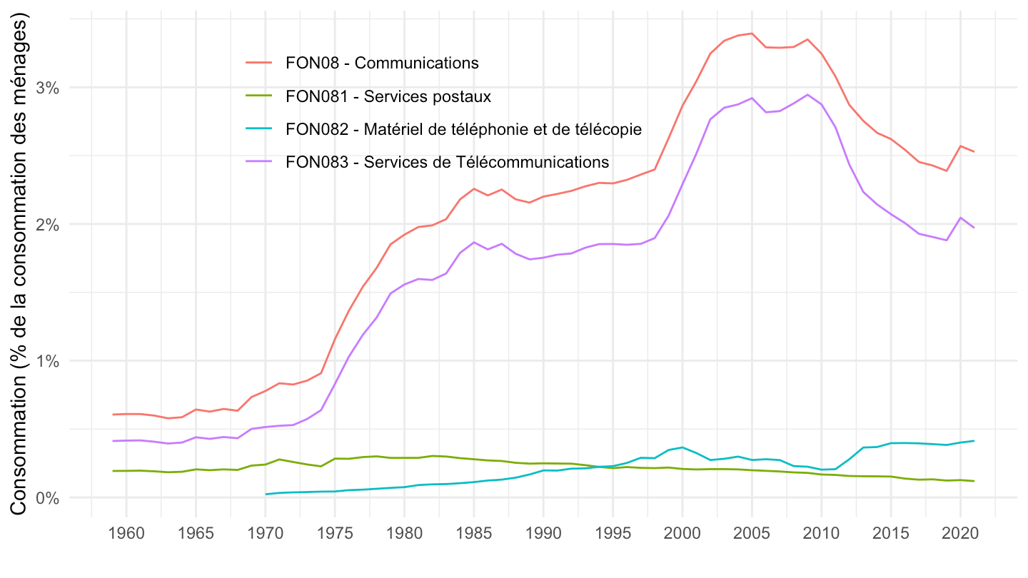

Définitions de la consommation

% du PIB

Code

`CNA-2014-CONSO-MEN` |>
  filter(CNA_PRODUIT %in% c("FONDEPHSI", "FONDEP", "FONTOTAL"),
         NATURE == "VALEUR_ABSOLUE",
         PRIX_REF == "VAL") %>%
  select_if(~ n_distinct(.) > 1) |>
  year_to_date() |>
  left_join(gdp, by = "date") |>
  
  ggplot() + theme_minimal() + ylab("Consommation (% du PIB)") + xlab("") +
  geom_line(aes(x = date, y = OBS_VALUE/(gdp), color = CNA_PRODUIT)) +
  theme(legend.title = element_blank(),
        legend.position = c(0.5, 0.5)) +
  scale_x_date(breaks = seq(1950, 2100, 5) |> paste0("-01-01") |> as.Date(),
               labels = date_format("%Y")) +
  
  scale_y_continuous(breaks = 0.01*seq(0, 100, 2),
                     labels = scales::percent_format(accuracy = 1))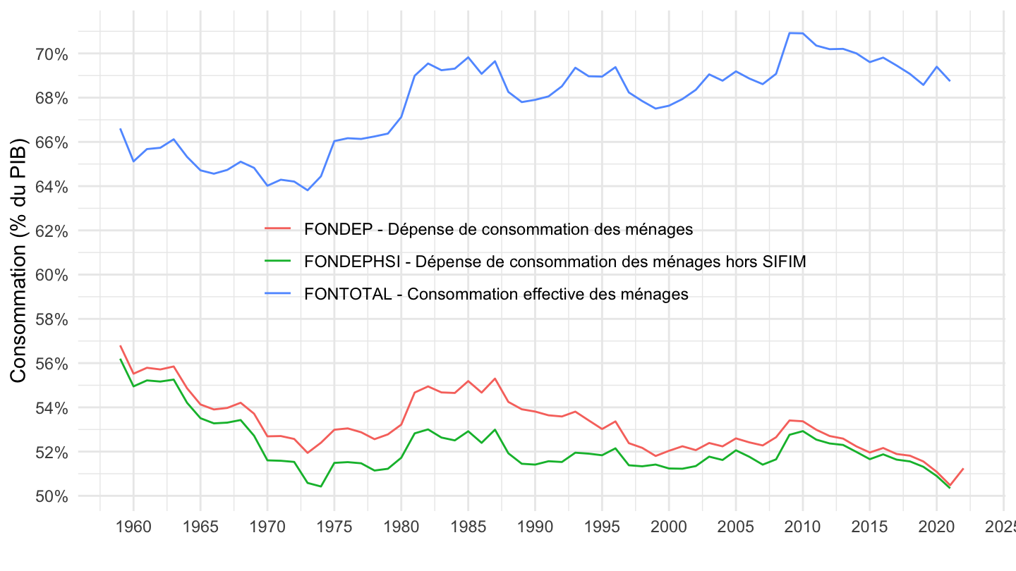

% de la conso finale

Code

`CNA-2014-CONSO-MEN` |>
  filter(CNA_PRODUIT %in% c("FONDEPHSI", "FONDEP", "FONTOTAL"),
         NATURE == "VALEUR_ABSOLUE",
         PRIX_REF == "VAL") %>%
  select_if(~ n_distinct(.) > 1) |>
  year_to_date() |>
  left_join(conso_finale_effective, by = "date") |>
  
  ggplot() + theme_minimal() + ylab("Consommation (% de la conso finale effective)") + xlab("") +
  geom_line(aes(x = date, y = OBS_VALUE/(conso_finale_effective), color = CNA_PRODUIT)) +
  theme(legend.title = element_blank(),
        legend.position = c(0.5, 0.5)) +
  scale_x_date(breaks = seq(1950, 2100, 5) |> paste0("-01-01") |> as.Date(),
               labels = date_format("%Y")) +
  
  scale_y_continuous(breaks = 0.01*seq(0, 100, 2),
                     labels = scales::percent_format(accuracy = 1))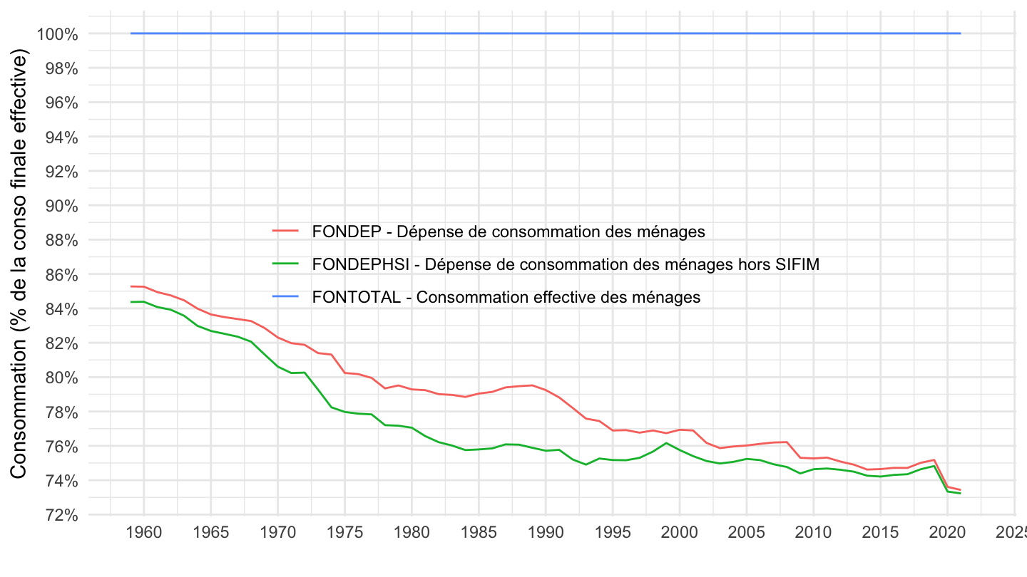

% de la consommation des ménages hors SIFIM

Code

`CNA-2014-CONSO-MEN` |>
  filter(CNA_PRODUIT %in% c("FONDEPHSI", "FONDEP", "FONTOTAL"),
         NATURE == "VALEUR_ABSOLUE",
         PRIX_REF == "VAL") %>%
  select_if(~ n_distinct(.) > 1) |>
  year_to_date() |>
  left_join(conso_menages, by = "date") |>
  
  ggplot() + theme_minimal() + ylab("Consommation (% de la consommation des ménages)") + xlab("") +
  geom_line(aes(x = date, y = OBS_VALUE/(conso_menages), color = CNA_PRODUIT)) +
  theme(legend.title = element_blank(),
        legend.position = c(0.5, 0.5)) +
  scale_x_date(breaks = seq(1950, 2100, 5) |> paste0("-01-01") |> as.Date(),
               labels = date_format("%Y")) +
  
  scale_y_continuous(breaks = 0.01*seq(0, 200, 5),
                     labels = scales::percent_format(accuracy = 1))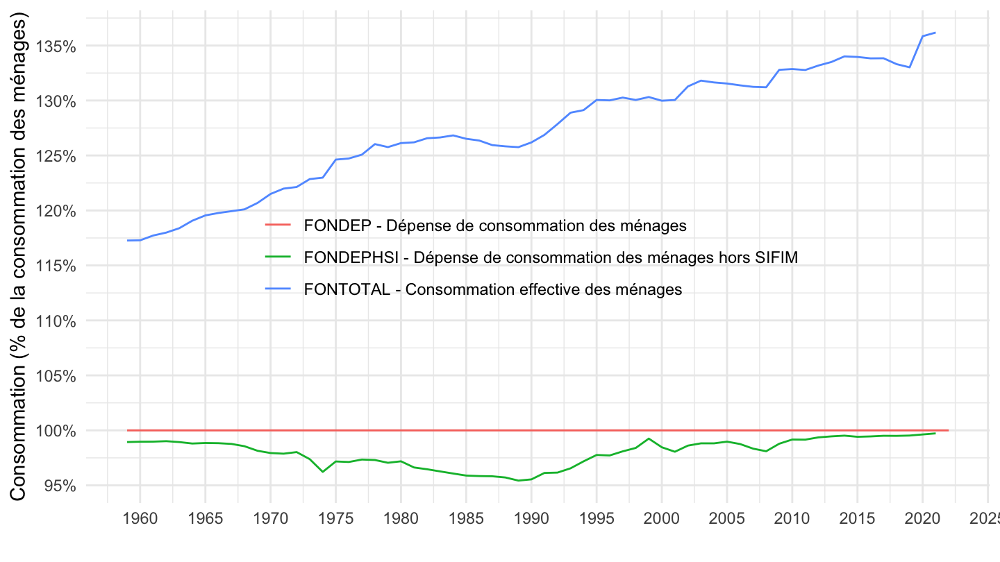

Santé

% du PIB

Code

`CNA-2014-CONSO-MEN` |>
  filter(CNA_PRODUIT %in% c("FON06", "FON1253", "FON142"),
         NATURE == "VALEUR_ABSOLUE",
         PRIX_REF == "VAL") %>%
  select_if(~ n_distinct(.) > 1) |>
  year_to_date() |>
  left_join(gdp, by = "date") |>
  
  ggplot() + theme_minimal() + ylab("Consommation (% du PIB)") + xlab("") +
  geom_line(aes(x = date, y = OBS_VALUE/(gdp), color = CNA_PRODUIT)) +
  theme(legend.title = element_blank(),
        legend.position = c(0.3, 0.91)) +
  scale_x_date(breaks = seq(1950, 2100, 5) |> paste0("-01-01") |> as.Date(),
               labels = date_format("%Y")) +
  
  scale_y_continuous(breaks = 0.01*seq(0, 100, 0.5),
                     labels = scales::percent_format(accuracy = 0.1))

% de la consommation finale effective

Code

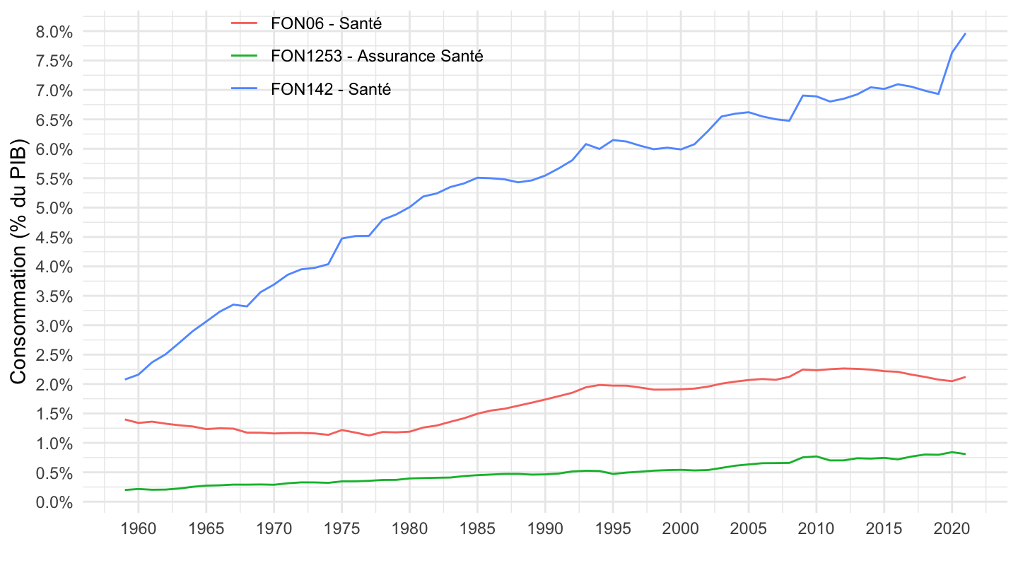
`CNA-2014-CONSO-MEN` |>
  filter(CNA_PRODUIT %in% c("FON06", "FON1253", "FON142"),
         NATURE == "VALEUR_ABSOLUE",
         PRIX_REF == "VAL") %>%
  select_if(~ n_distinct(.) > 1) |>
  year_to_date() |>
  left_join(conso_finale_effective, by = "date") |>
  
  ggplot() + theme_minimal() + ylab("Consommation (% de la consommation finale effective)") + xlab("") +
  geom_line(aes(x = date, y = OBS_VALUE/(conso_finale_effective), color = CNA_PRODUIT)) +
  theme(legend.title = element_blank(),
        legend.position = c(0.3, 0.91)) +
  scale_x_date(breaks = seq(1950, 2100, 5) |> paste0("-01-01") |> as.Date(),
               labels = date_format("%Y")) +
  
  scale_y_continuous(breaks = 0.01*seq(0, 100, 0.5),
                     labels = scales::percent_format(accuracy = 0.1))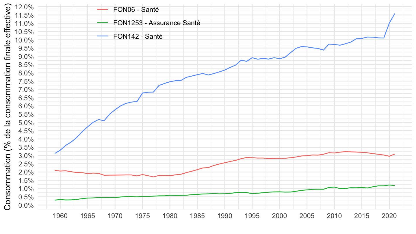

% de la consommation des ménages hors SIFIM

Code

`CNA-2014-CONSO-MEN` |>
  filter(CNA_PRODUIT %in% c("FON06", "FON1253", "FON142"),
         NATURE == "VALEUR_ABSOLUE",
         PRIX_REF == "VAL") %>%
  select_if(~ n_distinct(.) > 1) |>
  year_to_date() |>
  left_join(conso_menages, by = "date") |>
  
  ggplot() + theme_minimal() + ylab("Consommation (% de la consommation des ménages)") + xlab("") +
  geom_line(aes(x = date, y = OBS_VALUE/(conso_menages), color = CNA_PRODUIT)) +
  theme(legend.title = element_blank(),
        legend.position = c(0.3, 0.91)) +
  scale_x_date(breaks = seq(1950, 2100, 5) |> paste0("-01-01") |> as.Date(),
               labels = date_format("%Y")) +
  
  scale_y_continuous(breaks = 0.01*seq(0, 100, 0.5),
                     labels = scales::percent_format(accuracy = 0.1))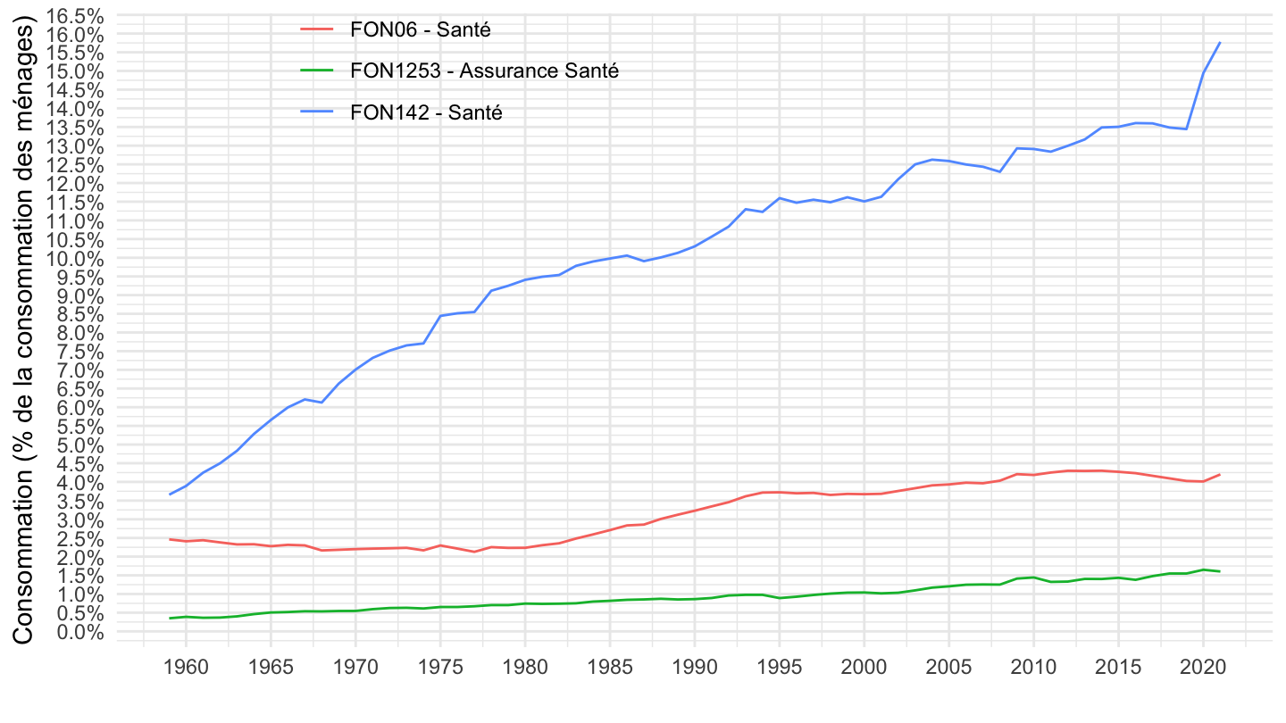

Loyers réels, loyers imputés

% du PIB

Code

`CNA-2014-CONSO-MEN` |>
  filter(CNA_PRODUIT %in% c("FON041", "FON042"),
         NATURE == "VALEUR_ABSOLUE",
         PRIX_REF == "VAL") %>%
  select_if(~ n_distinct(.) > 1) |>
  year_to_date() |>
  left_join(gdp, by = "date") |>
  
  ggplot() + theme_minimal() + ylab("Consommation (% du PIB)") + xlab("") +
  geom_line(aes(x = date, y = OBS_VALUE/(gdp), color = CNA_PRODUIT)) +
  theme(legend.title = element_blank(),
        legend.position = c(0.3, 0.91)) +
  scale_x_date(breaks = seq(1950, 2100, 5) |> paste0("-01-01") |> as.Date(),
               labels = date_format("%Y")) +
  
  scale_y_continuous(breaks = 0.01*seq(0, 100, 0.5),
                     labels = scales::percent_format(accuracy = 0.1))

% de la consommation finale effective

Code

`CNA-2014-CONSO-MEN` |>
  filter(CNA_PRODUIT %in% c("FON041", "FON042"),
         NATURE == "VALEUR_ABSOLUE",
         PRIX_REF == "VAL") %>%
  select_if(~ n_distinct(.) > 1) |>
  year_to_date() |>
  left_join(conso_finale_effective, by = "date") |>
  
  ggplot() + theme_minimal() + ylab("Consommation (% de la consommation)") + xlab("") +
  geom_line(aes(x = date, y = OBS_VALUE/(conso_finale_effective), color = CNA_PRODUIT)) +
  theme(legend.title = element_blank(),
        legend.position = c(0.3, 0.91)) +
  scale_x_date(breaks = seq(1950, 2100, 5) |> paste0("-01-01") |> as.Date(),
               labels = date_format("%Y")) +
  
  scale_y_continuous(breaks = 0.01*seq(0, 100, 0.5),
                     labels = scales::percent_format(accuracy = 0.1))

% de la consommation des ménages hors SIFIM

Tous

Code

`CNA-2014-CONSO-MEN` |>
  filter(CNA_PRODUIT %in% c("FON041", "FON042"),
         NATURE == "VALEUR_ABSOLUE",
         PRIX_REF == "VAL") %>%
  select_if(~ n_distinct(.) > 1) |>
  year_to_date() |>
  left_join(conso_menages, by = "date") |>
  
  ggplot() + theme_minimal() + ylab("Consommation (% de la consommation)") + xlab("") +
  geom_line(aes(x = date, y = OBS_VALUE/(conso_menages), color = CNA_PRODUIT)) +
  theme(legend.title = element_blank(),
        legend.position = c(0.3, 0.91)) +
  scale_x_date(breaks = seq(1950, 2100, 5) |> paste0("-01-01") |> as.Date(),
               labels = date_format("%Y")) +
  
  scale_y_continuous(breaks = 0.01*seq(0, 100, 0.5),
                     labels = scales::percent_format(accuracy = 0.1))

-2020

Code

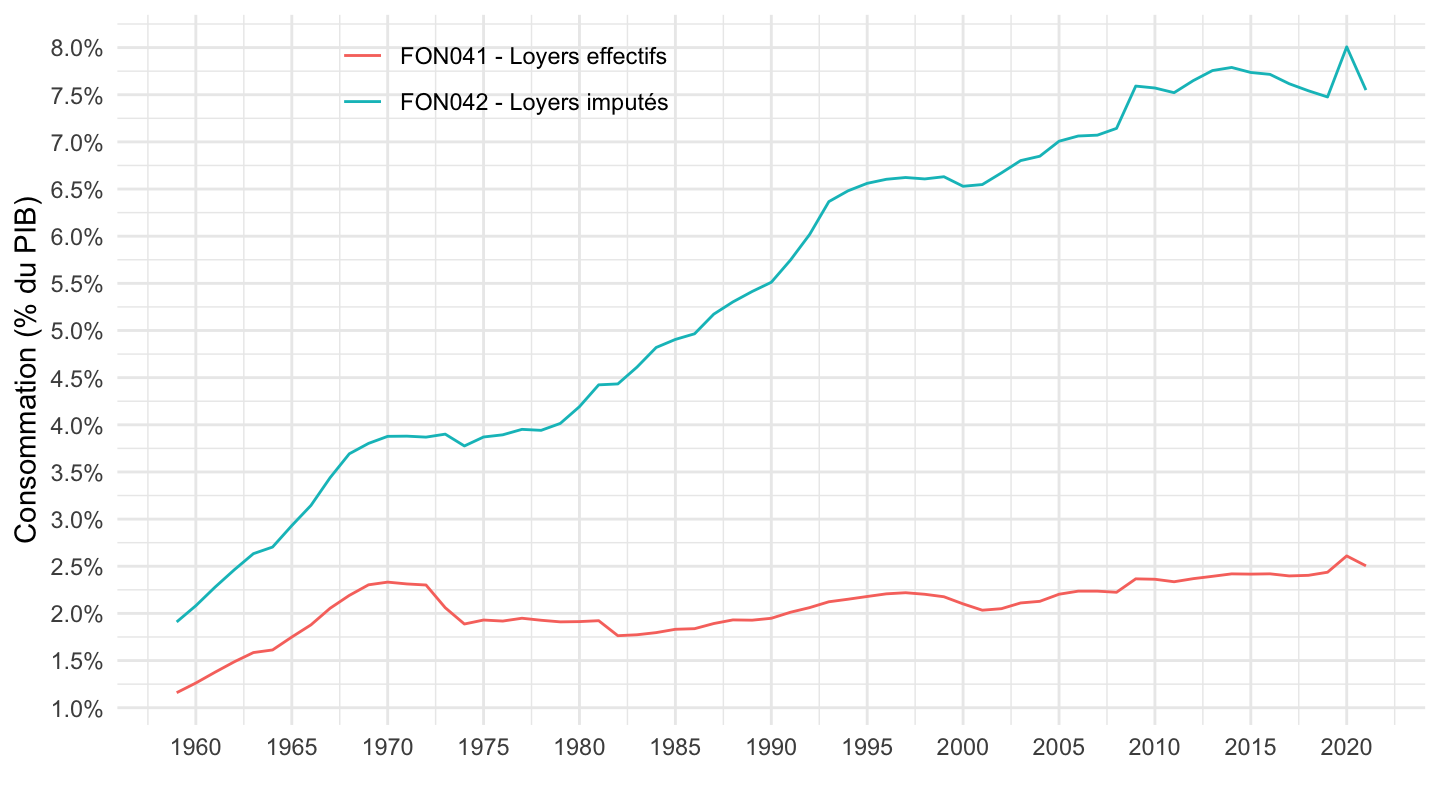
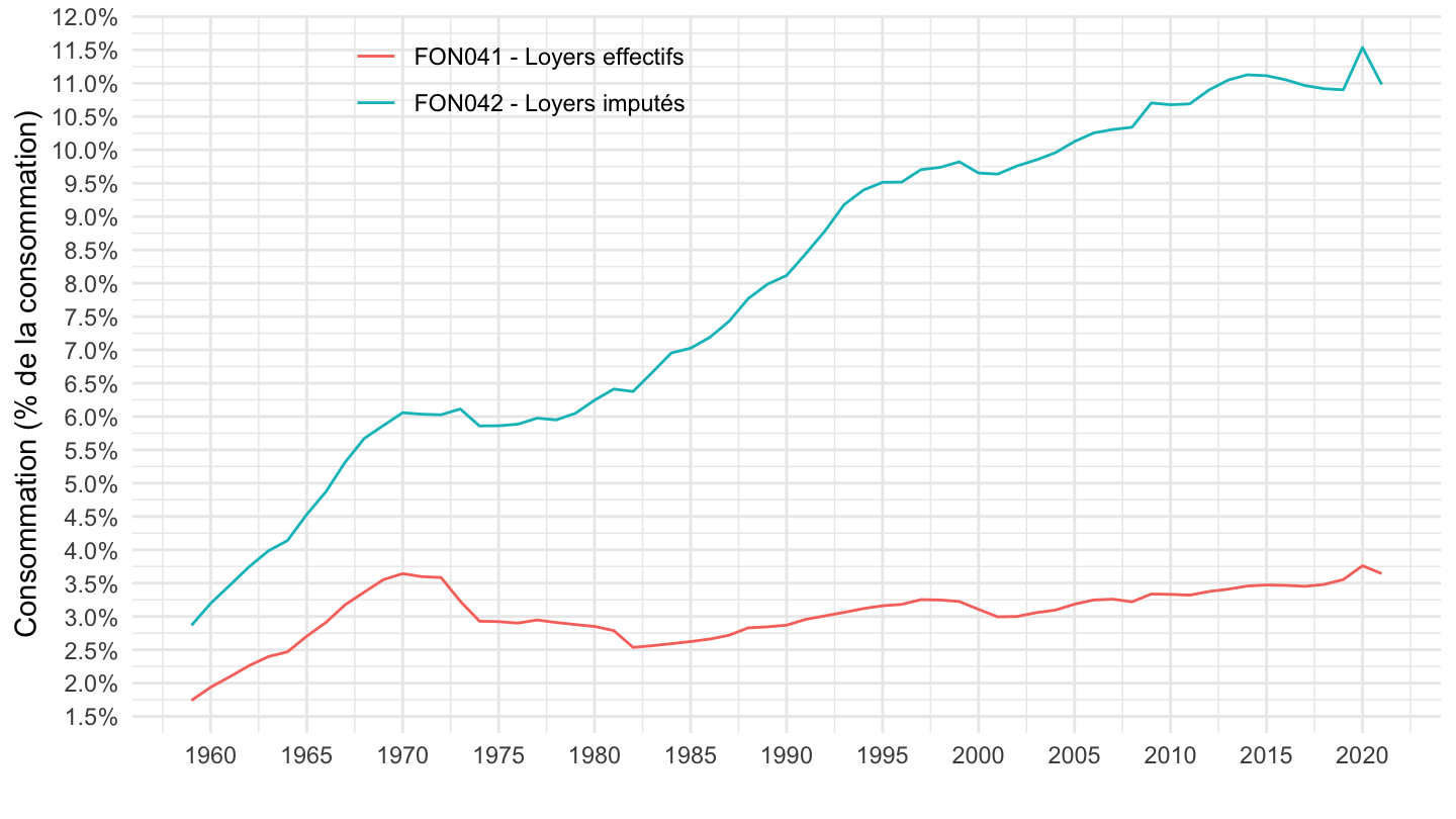
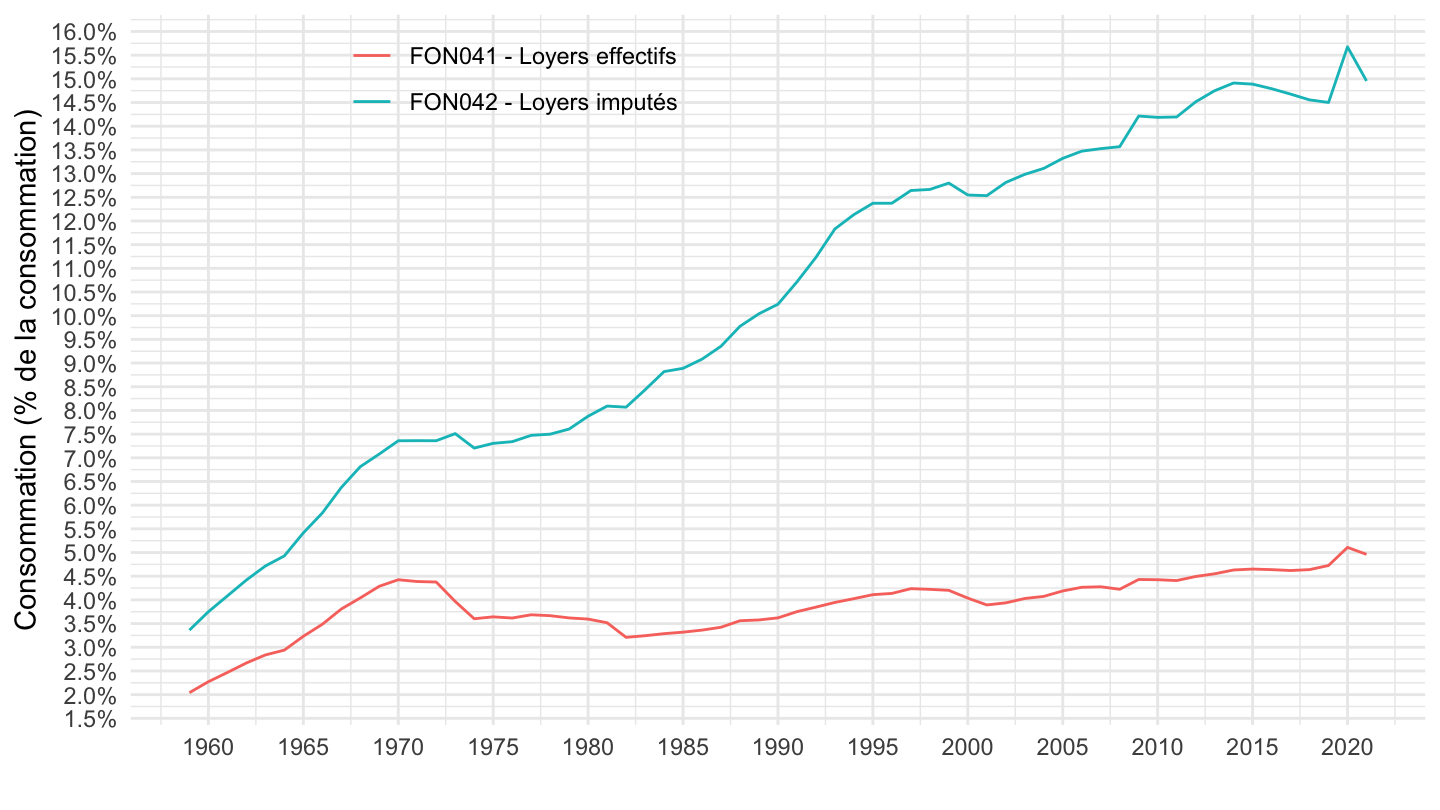
`CNA-2014-CONSO-MEN` |>
  filter(CNA_PRODUIT %in% c("FON041", "FON042"),
         NATURE == "VALEUR_ABSOLUE",
         PRIX_REF == "VAL") %>%
  select_if(~ n_distinct(.) > 1) |>
  year_to_date() |>
  left_join(conso_menages, by = "date") |>
  
  filter(date <= as.Date("2020-01-01")) |>
  ggplot() + theme_minimal() + ylab("Consommation de loyers\n% de la consommation des ménages hors SIFIM") + xlab("") +
  geom_line(aes(x = date, y = OBS_VALUE/(conso_menages), color = CNA_PRODUIT)) +
  theme(legend.title = element_blank(),
        legend.position = c(0.3, 0.91)) +
  scale_x_date(breaks = seq(1950, 2100, 5) |> paste0("-01-01") |> as.Date(),
               labels = date_format("%Y")) +
  
  scale_y_continuous(breaks = 0.01*seq(0, 100, 1),
                     labels = scales::percent_format(accuracy = 1))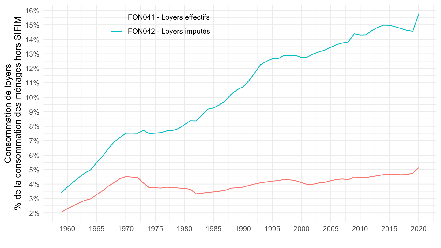

Tables 2020

Tous

Code

`CNA-2014-CONSO-MEN` |>
  filter(TIME_PERIOD == "2020",
         OPERATION == "P4") |>
  
  select_if(function(col) length(unique(col)) > 1) |>
  arrange(CNA_PRODUIT) |>
  select(CNA_PRODUIT, CNA_PRODUIT, UNIT_MEASURE, OBS_VALUE) |>
  spread(UNIT_MEASURE, OBS_VALUE) |>
  print_table_conditional()

Tables 2019

Tous

Code

`CNA-2014-CONSO-MEN` |>
  filter(TIME_PERIOD == "2019",
         OPERATION == "P4") |>
  
  select_if(function(col) length(unique(col)) > 1) |>
  arrange(CNA_PRODUIT) |>
  select(CNA_PRODUIT, CNA_PRODUIT, UNIT_MEASURE, OBS_VALUE) |>
  spread(UNIT_MEASURE, OBS_VALUE) |>
  print_table_conditional()

A10

Code

`CNA-2014-CONSO-MEN` |>
  filter(grepl("A10", CNA_PRODUIT),
         TIME_PERIOD == "2019") |>
  
  arrange(CNA_PRODUIT) |>
  select(CNA_PRODUIT, CNA_PRODUIT, UNIT_MEASURE, OBS_VALUE) |>
  spread(UNIT_MEASURE, OBS_VALUE) |>
  print_table_conditional()

CNA_PRODUIT	EUR2014	EUROS_COURANTS	SO
A10-AZ	31388	37961	120.9
A10-BE	578729	590072	102.0
A10-FZ	18355	19949	108.7
A10-GI	149994	161801	107.9
A10-JZ	47850	46810	97.8
A10-KZ	63668	69731	109.5
A10-LZ	255168	258910	101.5
A10-MN	27674	27870	100.7
A10-OQ	370420	384739	103.9
A10-RU	87036	88859	102.1

A17

Code

`CNA-2014-CONSO-MEN` |>
  filter(grepl("A17", CNA_PRODUIT),
         TIME_PERIOD == "2019") |>
  
  arrange(CNA_PRODUIT) |>
  select(CNA_PRODUIT, CNA_PRODUIT, UNIT_MEASURE, OBS_VALUE) |>
  spread(UNIT_MEASURE, OBS_VALUE) |>
  print_table_conditional()

CNA_PRODUIT	EUR2014	EUROS_COURANTS	SO
A17-AZ	31388	37961	120.9
A17-C1	175245	186526	106.4
A17-C2	46549	49859	107.1
A17-C3	38603	32220	83.5
A17-C4	73249	75510	103.1
A17-C5	192860	187893	97.4
A17-DE	52498	58064	110.6
A17-FZ	18355	19949	108.7
A17-GZ	14655	16063	109.6
A17-HZ	45388	48046	105.9
A17-IZ	89924	97692	108.6
A17-JZ	47850	46810	97.8
A17-KZ	63668	69731	109.5
A17-LZ	255168	258910	101.5
A17-MN	27674	27870	100.7
A17-OQ	370420	384739	103.9
A17-RU	87036	88859	102.1

A38

Code

`CNA-2014-CONSO-MEN` |>
  filter(grepl("A38", CNA_PRODUIT),
         TIME_PERIOD == "2019") |>
  
  arrange(CNA_PRODUIT) |>
  select(CNA_PRODUIT, CNA_PRODUIT, UNIT_MEASURE, OBS_VALUE) |>
  spread(UNIT_MEASURE, OBS_VALUE) |>
  print_table_conditional()

A88

Code

`CNA-2014-CONSO-MEN` |>
  filter(grepl("A88", CNA_PRODUIT),
         TIME_PERIOD == "2019") |>
  
  arrange(CNA_PRODUIT) |>
  select(CNA_PRODUIT, CNA_PRODUIT, UNIT_MEASURE, OBS_VALUE) |>
  spread(UNIT_MEASURE, OBS_VALUE) |>
  print_table_conditional()

DUR - Par durabilité

Code

`CNA-2014-CONSO-MEN` |>
  filter(grepl("DUR", CNA_PRODUIT),
         TIME_PERIOD == "2019") |>
  
  arrange(CNA_PRODUIT) |>
  select(CNA_PRODUIT, CNA_PRODUIT, UNIT_MEASURE, OBS_VALUE) |>
  spread(UNIT_MEASURE, OBS_VALUE) |>
  print_table_conditional()

CNA_PRODUIT	EUR2014	EUROS_COURANTS	SO
DUR1	113326	109143	96.3
DUR11	40467	41159	101.7
DUR12	15625	15550	99.5
DUR13	7923	7221	91.1
DUR14	49365	45214	91.6
DUR2	94188	92842	98.6
DUR21	47808	47423	99.2
DUR22	46389	45419	97.9
DUR3	384514	406918	105.8
DUR31	180554	192568	106.7
DUR32	91241	99623	109.2
DUR33	112671	114727	101.8
DUR4	1038362	1077799	103.8
DUR41	252449	256083	101.5
DUR42	169548	171654	101.2
DUR43	76222	77221	101.3
DUR44	90026	97725	108.6
DUR45	107062	110931	103.6
DUR46	342942	364184	106.2
DUR5	-14495	-15056	103.9
DURTOTAL	1615941	1671646	103.4

FON

Code

`CNA-2014-CONSO-MEN` |>
  filter(grepl("FON", CNA_PRODUIT),
         TIME_PERIOD == "2019") |>
  
  arrange(CNA_PRODUIT) |>
  select(CNA_PRODUIT, CNA_PRODUIT, UNIT_MEASURE, OBS_VALUE) |>
  spread(UNIT_MEASURE, OBS_VALUE) |>
  print_table_conditional()

GG

Code

`CNA-2014-CONSO-MEN` |>
  filter(grepl("GG", CNA_PRODUIT),
         TIME_PERIOD == "2019") |>
  
  arrange(CNA_PRODUIT) |>
  select(CNA_PRODUIT, CNA_PRODUIT, UNIT_MEASURE, OBS_VALUE) |>
  spread(UNIT_MEASURE, OBS_VALUE) |>
  print_table_conditional()

Loyers réels, loyers imputés, Tous

Montant

1990-2020

Code

`CNA-2014-CONSO-MEN` |>
  filter(CNA_PRODUIT %in% c("FON041", "FON042", "NNTOTAL"),
         NATURE == "VALEUR_ABSOLUE",
         PRIX_REF == "VAL",
         OPERATION %in% c("P4")) %>%
  select_if(~ n_distinct(.) > 1) |>
  year_to_date() |>
  filter(date >= as.Date("1990-01-01"),
         date <= as.Date("2020-01-01")) |>
  
  group_by(CNA_PRODUIT) |>
  arrange(date) |>
  mutate(OBS_VALUE = 100*OBS_VALUE/OBS_VALUE[1]) |>
  ggplot() + theme_minimal() + ylab("Consommation en valeur") + xlab("") +
  geom_line(aes(x = date, y = OBS_VALUE, color = CNA_PRODUIT)) +
  theme(legend.title = element_blank(),
        legend.position = c(0.3, 0.8)) +
  scale_x_date(breaks = seq(1950, 2100, 5) |> paste0("-01-01") |> as.Date(),
               labels = date_format("%Y")) +
  
  scale_y_log10(breaks = seq(80, 1000, 10)) +
  geom_label(data = . %>% filter(date == max(date)),
             aes(x = date, y = OBS_VALUE, label = round(OBS_VALUE, 1), color = CNA_PRODUIT), show.legend = F)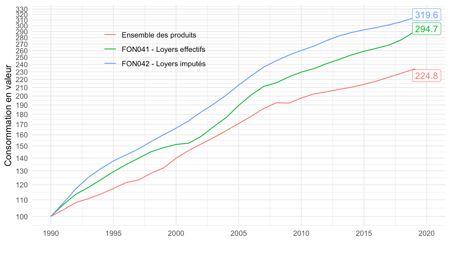

PCH (Prix chaîné année de base (non équilibré))

1990-2020

Code

`CNA-2014-CONSO-MEN` |>
  filter(CNA_PRODUIT %in% c("FON041", "FON042", "NNTOTAL"),
         NATURE == "VALEUR_ABSOLUE",
         PRIX_REF == "PCH",
         OPERATION %in% c("P4")) %>%
  select_if(~ n_distinct(.) > 1) |>
  year_to_date() |>
  filter(date >= as.Date("1990-01-01"),
         date <= as.Date("2020-01-01")) |>
  
  group_by(CNA_PRODUIT) |>
  arrange(date) |>
  mutate(OBS_VALUE = 100*OBS_VALUE/OBS_VALUE[1]) |>
  ggplot() + theme_minimal() + ylab("Consommation en volume\nPrix chaîné année de base") + xlab("") +
  geom_line(aes(x = date, y = OBS_VALUE, color = CNA_PRODUIT)) +
  theme(legend.title = element_blank(),
        legend.position = c(0.3, 0.8)) +
  scale_x_date(breaks = seq(1950, 2100, 5) |> paste0("-01-01") |> as.Date(),
               labels = date_format("%Y")) +
  
  scale_y_log10(breaks = seq(80, 1000, 5)) +
  geom_label(data = . %>% filter(date == max(date)),
             aes(x = date, y = OBS_VALUE, label = round(OBS_VALUE, 1), color = CNA_PRODUIT), show.legend = F)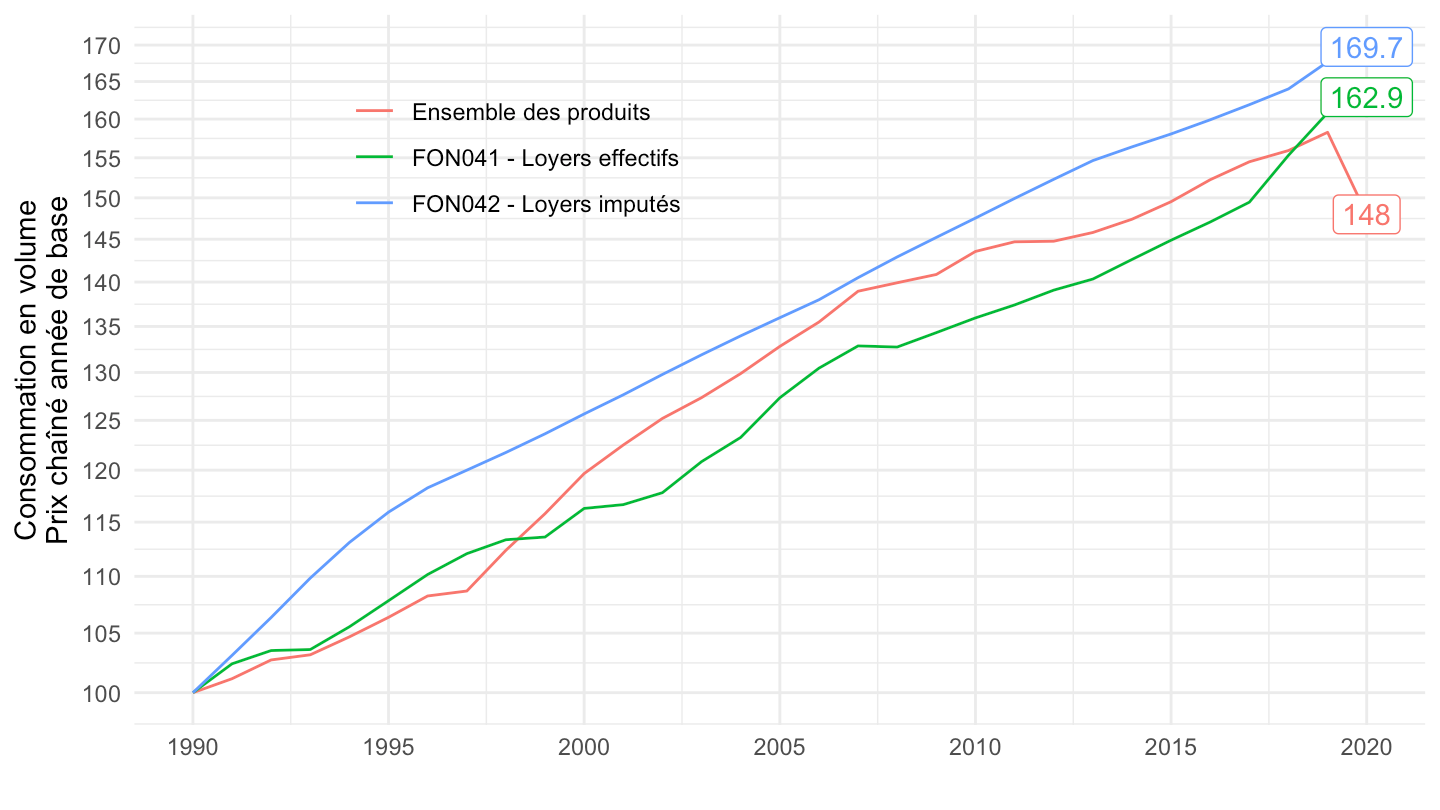

Remontées mécaniques

Code

`CNA-2014-CONSO-MEN` |>
  filter(grepl("remontées", TITLE_FR)) |>
  year_to_date() |>
  arrange(date) |>
  ggplot() + theme_minimal() + xlab("") + ylab("") +
  geom_line(aes(x = date, y = OBS_VALUE, color = UNIT_MEASURE)) +
  scale_x_date(breaks = seq(1960, 2100, 5) |> paste0("-01-01") |> as.Date(),
               labels = date_format("%Y")) +
  scale_y_log10(breaks = c(1, 5, 10, 20, 50, 100, 200, 300, 500, 1000)) +
  
  theme(legend.position = c(0.2, 0.9),
        legend.title = element_blank())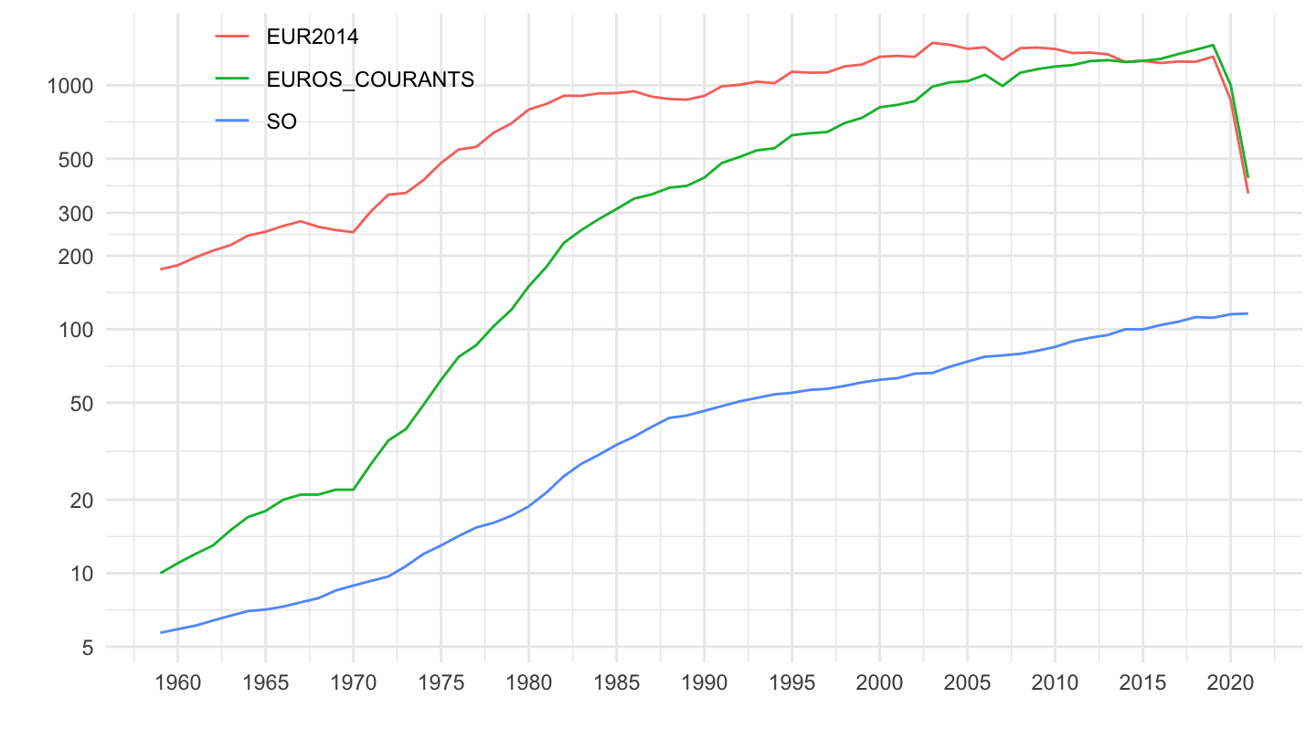

Loyers effectifs, loyers imputés

1959-

Code

`CNA-2014-CONSO-MEN` |>
  filter(CNA_PRODUIT %in% c("FON042", "NNTOTAL", "FON041"),
         NATURE == "INDICE",
         OPERATION == "P4") |>
  
  year_to_date() |>
  arrange(date) |>
  group_by(CNA_PRODUIT) |>
  arrange(date) |>
  mutate(OBS_VALUE = 100*OBS_VALUE/OBS_VALUE[1]) |>
  ggplot() + theme_minimal() + xlab("") + ylab("") +
  geom_line(aes(x = date, y = OBS_VALUE, color = CNA_PRODUIT)) +
  scale_x_date(breaks = seq(1960, 2100, 5) |> paste0("-01-01") |> as.Date(),
               labels = date_format("%Y")) +
  scale_y_log10(breaks = c(100, 200, 300, 500, 1000, 2000)) +
  #
  theme(legend.position = c(0.2, 0.9),
        legend.title = element_blank())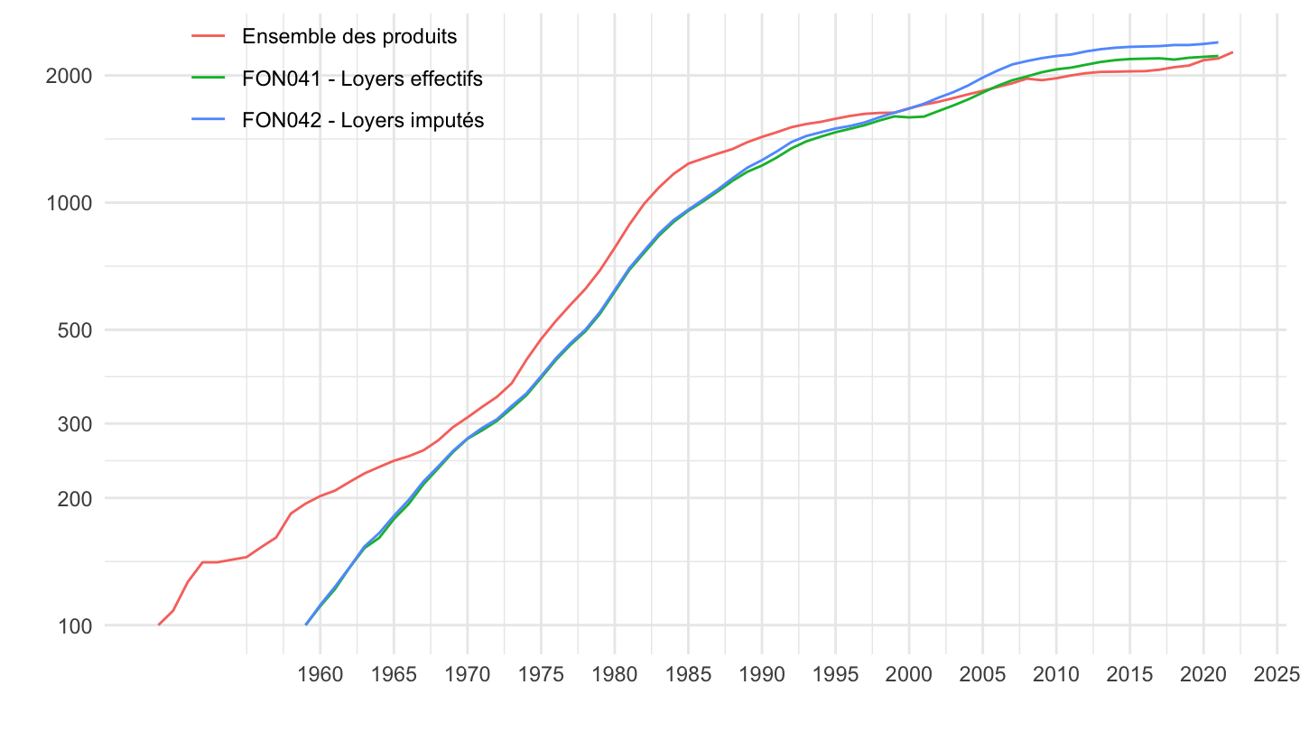

1990-

Code

`CNA-2014-CONSO-MEN` |>
  filter(CNA_PRODUIT %in% c("FON042", "NNTOTAL", "FON041"),
         NATURE == "INDICE",
         OPERATION == "P4") |>
  
  year_to_date() |>
  filter(date >= as.Date("1990-01-01")) |>
  group_by(CNA_PRODUIT) |>
  arrange(date) |>
  mutate(OBS_VALUE = 100*OBS_VALUE/OBS_VALUE[1]) |>
  ggplot() + theme_minimal() + xlab("") + ylab("") +
  geom_line(aes(x = date, y = OBS_VALUE, color = CNA_PRODUIT)) +
  scale_x_date(breaks = seq(1960, 2100, 5) |> paste0("-01-01") |> as.Date(),
               labels = date_format("%Y")) +
  scale_y_log10(breaks = seq(100, 300, 10)) +
  #
  theme(legend.position = c(0.25, 0.9),
        legend.title = element_blank())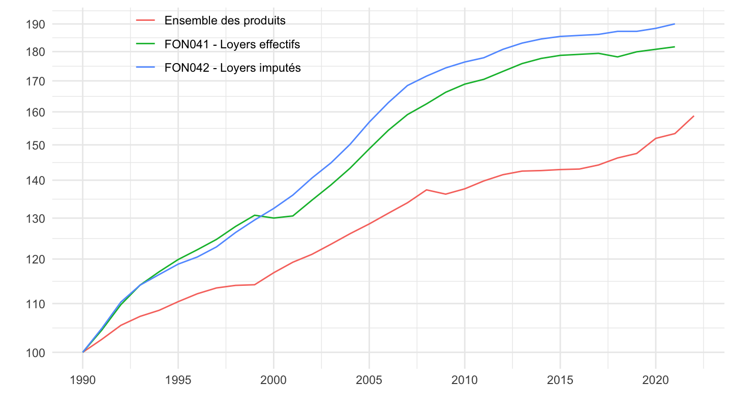

1992-

Code

`CNA-2014-CONSO-MEN` |>
  filter(CNA_PRODUIT %in% c("FON042", "FON041", "NNTOTAL"),
         NATURE == "INDICE",
         OPERATION == "P4") |>
  
  year_to_date() |>
  bind_rows(baguette) |>
  filter(date >= as.Date("1992-01-01")) |>
  group_by(CNA_PRODUIT) |>
  arrange(date) |>
  mutate(OBS_VALUE = 100*OBS_VALUE/OBS_VALUE[1]) |>
  ggplot() + theme_minimal() + xlab("") + ylab("") +
  geom_line(aes(x = date, y = OBS_VALUE, color = Cna_produit)) +
  scale_x_date(breaks = seq(1960, 2100, 2) |> paste0("-01-01") |> as.Date(),
               labels = date_format("%Y")) +
  scale_y_log10(breaks = seq(100, 300, 10)) +
  
  theme(legend.position = c(0.25, 0.9),
        legend.title = element_blank())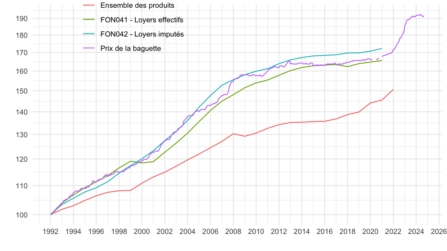

1996-

Code

`CNA-2014-CONSO-MEN` |>
  filter(CNA_PRODUIT %in% c("FON042", "FON041", "NNTOTAL"),
         NATURE == "INDICE",
         OPERATION == "P4") |>
  
  year_to_date() |>
  bind_rows(baguette) |>
  filter(date >= as.Date("1996-01-01")) |>
  group_by(CNA_PRODUIT) |>
  arrange(date) |>
  mutate(OBS_VALUE = 100*OBS_VALUE/OBS_VALUE[1]) |>
  ggplot() + theme_minimal() + xlab("") + ylab("") +
  geom_line(aes(x = date, y = OBS_VALUE, color = Cna_produit)) +
  scale_x_date(breaks = seq(1960, 2100, 2) |> paste0("-01-01") |> as.Date(),
               labels = date_format("%Y")) +
  scale_y_log10(breaks = seq(100, 300, 10)) +
  #
  theme(legend.position = c(0.25, 0.9),
        legend.title = element_blank())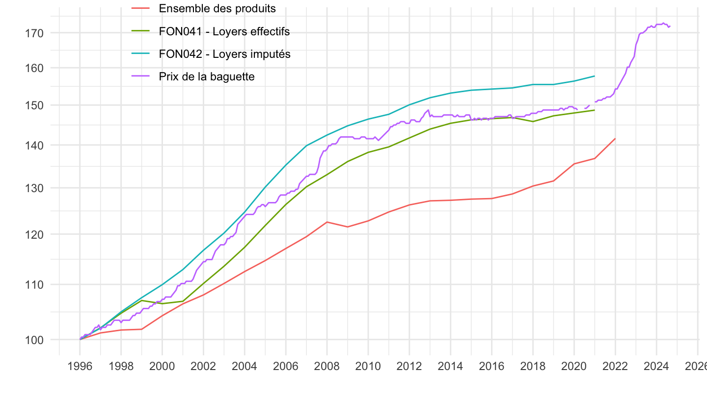

1998-

Code

`CNA-2014-CONSO-MEN` |>
  filter(CNA_PRODUIT %in% c("FON042", "FON041", "NNTOTAL"),
         NATURE == "INDICE",
         OPERATION == "P4") |>
  
  year_to_date() |>
  filter(date >= as.Date("1998-01-01")) |>
  group_by(CNA_PRODUIT) |>
  arrange(date) |>
  mutate(OBS_VALUE = 100*OBS_VALUE/OBS_VALUE[1]) |>
  ggplot() + theme_minimal() + xlab("") + ylab("") +
  geom_line(aes(x = date, y = OBS_VALUE, color = CNA_PRODUIT)) +
  scale_x_date(breaks = seq(1960, 2100, 2) |> paste0("-01-01") |> as.Date(),
               labels = date_format("%Y")) +
  scale_y_log10(breaks = seq(100, 300, 10)) +
  
  theme(legend.position = c(0.25, 0.9),
        legend.title = element_blank())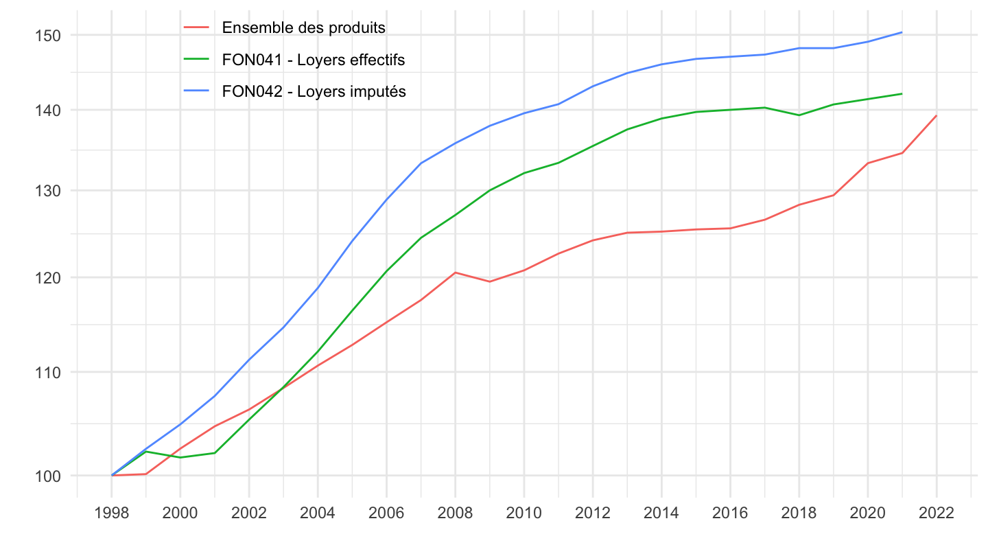

FON

Code

`CNA-2014-CONSO-MEN` |>
  filter(CNA_PRODUIT %in% c("FON042", "FON041"),
         NATURE == "INDICE") |>
  
  year_to_date() |>
  ggplot() + theme_minimal() + xlab("") + ylab("") +
  geom_line(aes(x = date, y = OBS_VALUE, color = CNA_PRODUIT)) +
  scale_x_date(breaks = seq(1960, 2100, 5) |> paste0("-01-01") |> as.Date(),
               labels = date_format("%Y")) +
  scale_y_log10(breaks = c(1, 5, 10, 20, 50, 100, 200, 300, 500, 1000)) +
  
  theme(legend.position = c(0.2, 0.9),
        legend.title = element_blank())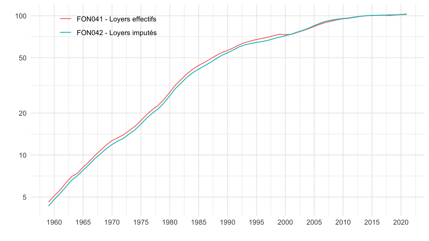

GG

Code

`CNA-2014-CONSO-MEN` |>
  filter(CNA_PRODUIT %in% c("GGL68I", "GGL68R", "GGL68A"),
         NATURE == "INDICE") |>
  
  year_to_date() |>
  ggplot() + theme_minimal() + xlab("") + ylab("") +
  geom_line(aes(x = date, y = OBS_VALUE, color = CNA_PRODUIT)) +
  scale_x_date(breaks = seq(1960, 2100, 5) |> paste0("-01-01") |> as.Date(),
               labels = date_format("%Y")) +
  scale_y_log10(breaks = c(1, 5, 10, 20, 50, 100, 200, 300, 500, 1000)) +
  
  theme(legend.position = c(0.55, 0.15),
        legend.title = element_blank())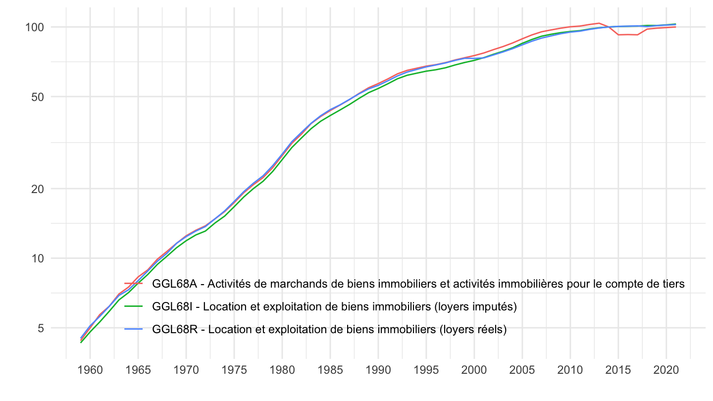

Immobilier, Loyers

1992-

Code

`CNA-2014-CONSO-MEN` |>
  filter(CNA_PRODUIT %in% c("FON042", "FON041", "NNTOTAL"),
         NATURE == "INDICE",
         OPERATION == "P4") |>
  
  year_to_date() |>
  filter(date >= as.Date("1992-01-01")) |>
  group_by(CNA_PRODUIT) |>
  arrange(date) |>
  mutate(OBS_VALUE = 100*OBS_VALUE/OBS_VALUE[1]) |>
  bind_rows(baguette) |>
  ggplot() + theme_minimal() + xlab("") + ylab("") +
  geom_line(aes(x = date, y = OBS_VALUE, color = Cna_produit)) +
  scale_x_date(breaks = seq(1960, 2100, 2) |> paste0("-01-01") |> as.Date(),
               labels = date_format("%Y")) +
  scale_y_log10(breaks = seq(100, 300, 10)) +
  
  theme(legend.position = c(0.25, 0.9),
        legend.title = element_blank())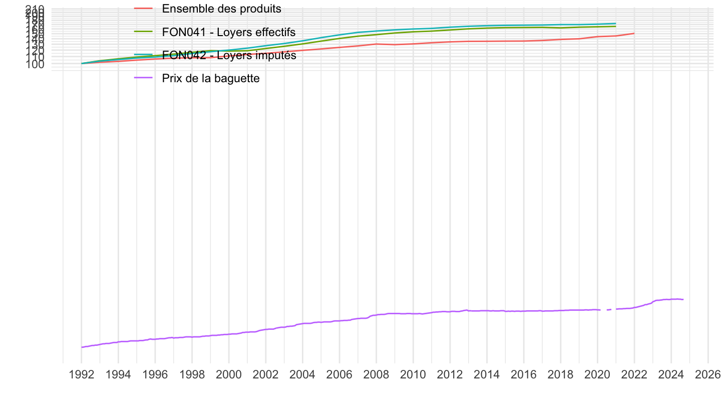

Activités immobilières, Ensemble

1959-

Code

`CNA-2014-CONSO-MEN` |>
  filter(CNA_PRODUIT %in% c("A88-68", "NNTOTAL"),
         NATURE == "INDICE",
         OPERATION == "P4") |>
  
  year_to_date() |>
  arrange(date) |>
  group_by(CNA_PRODUIT) |>
  arrange(date) |>
  mutate(OBS_VALUE = 100*OBS_VALUE/OBS_VALUE[1]) |>
  ggplot() + theme_minimal() + xlab("") + ylab("") +
  geom_line(aes(x = date, y = OBS_VALUE, color = CNA_PRODUIT)) +
  scale_x_date(breaks = seq(1960, 2100, 5) |> paste0("-01-01") |> as.Date(),
               labels = date_format("%Y")) +
  scale_y_log10(breaks = c(100, 200, 300, 500, 1000, 2000)) +
  
  theme(legend.position = c(0.2, 0.9),
        legend.title = element_blank())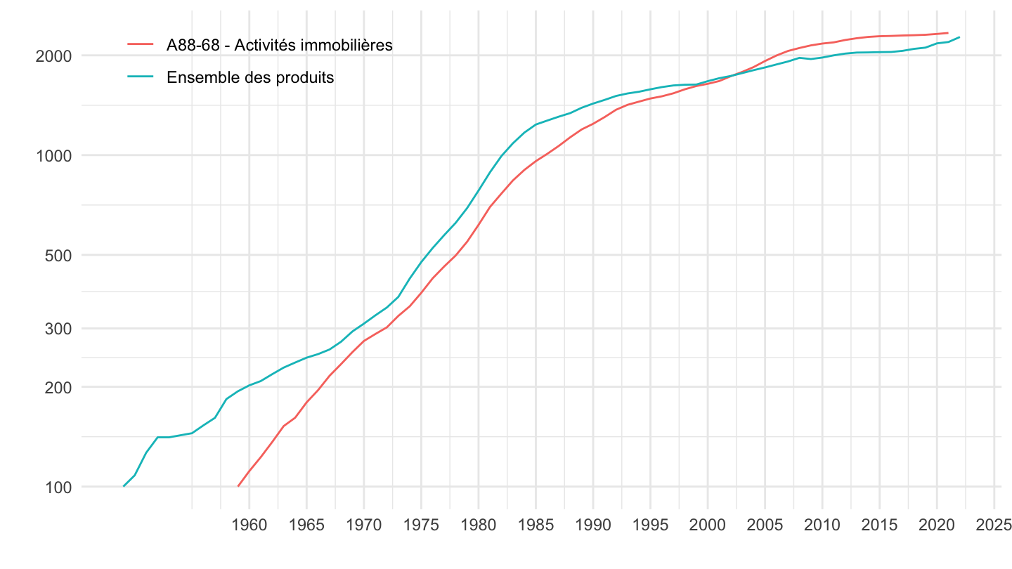

1990-

Code

`CNA-2014-CONSO-MEN` |>
  filter(CNA_PRODUIT %in% c("A88-68", "NNTOTAL"),
         NATURE == "INDICE",
         OPERATION == "P4") |>
  
  year_to_date() |>
  filter(date >= as.Date("1990-01-01")) |>
  group_by(CNA_PRODUIT) |>
  arrange(date) |>
  mutate(OBS_VALUE = 100*OBS_VALUE/OBS_VALUE[1]) |>
  ggplot() + theme_minimal() + xlab("") + ylab("") +
  geom_line(aes(x = date, y = OBS_VALUE, color = CNA_PRODUIT)) +
  scale_x_date(breaks = seq(1960, 2100, 5) |> paste0("-01-01") |> as.Date(),
               labels = date_format("%Y")) +
  scale_y_log10(breaks = seq(100, 300, 10)) +
  
  theme(legend.position = c(0.25, 0.9),
        legend.title = element_blank())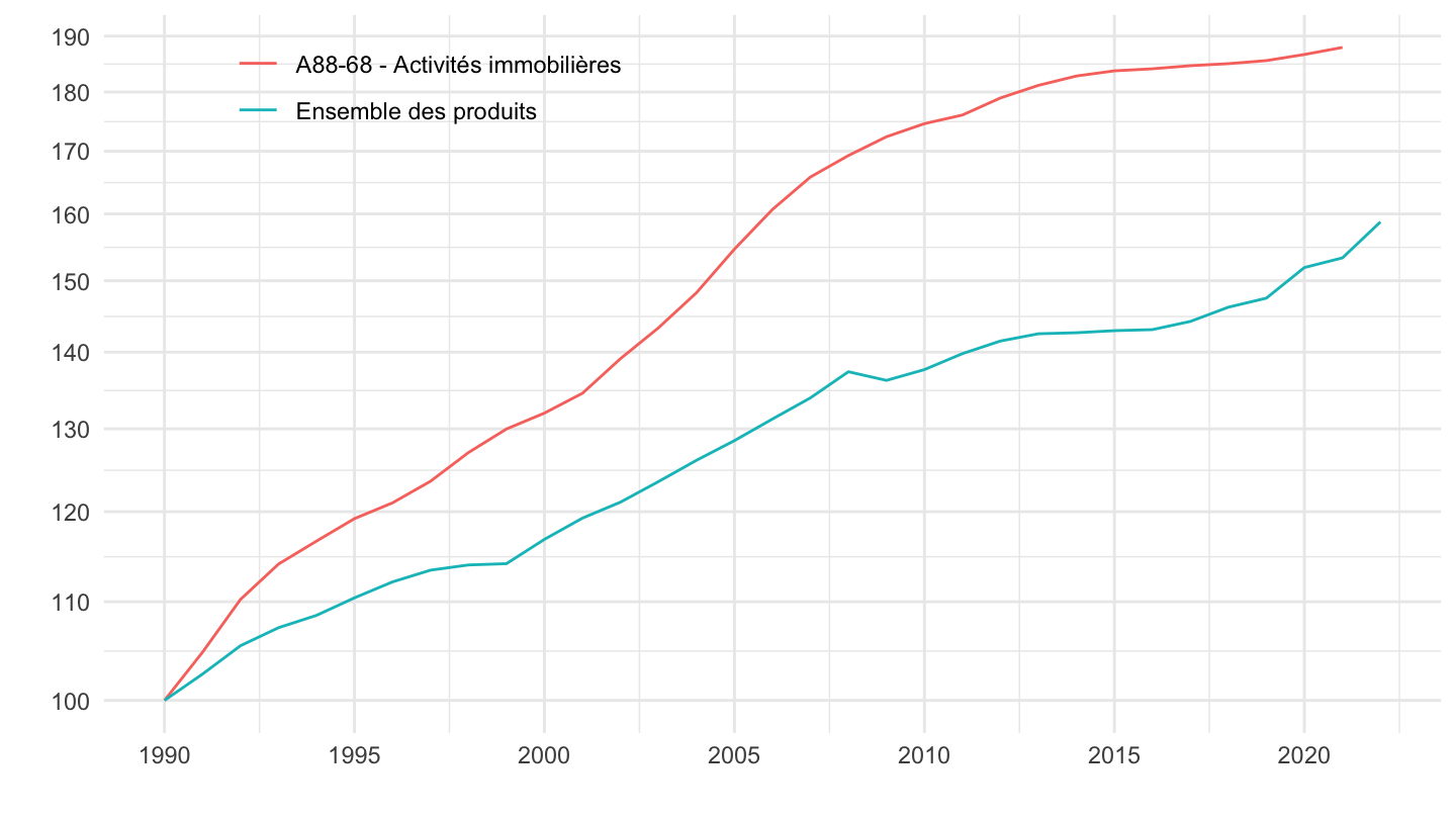

2000-

Code

`CNA-2014-CONSO-MEN` |>
  filter(CNA_PRODUIT %in% c("A88-68", "NNTOTAL"),
         NATURE == "INDICE",
         OPERATION == "P4") |>
  
  year_to_date() |>
  filter(date >= as.Date("2000-01-01")) |>
  group_by(CNA_PRODUIT) |>
  arrange(date) |>
  mutate(OBS_VALUE = 100*OBS_VALUE/OBS_VALUE[1]) |>
  ggplot() + theme_minimal() + xlab("") + ylab("") +
  geom_line(aes(x = date, y = OBS_VALUE, color = CNA_PRODUIT)) +
  scale_x_date(breaks = seq(1960, 2100, 2) |> paste0("-01-01") |> as.Date(),
               labels = date_format("%Y")) +
  scale_y_log10(breaks = seq(100, 300, 10)) +
  
  theme(legend.position = c(0.25, 0.9),
        legend.title = element_blank())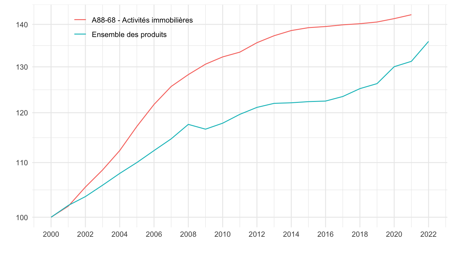

Comparaisons

Immobilier, Pain, Ensemble

Code

`CNA-2014-CONSO-MEN` |>
  filter(CNA_PRODUIT %in% c("A88-68", "HIHC10G1A", "NNTOTAL", "FON0111"),
         NATURE == "INDICE",
         OPERATION == "P4") |>
  
  year_to_date() |>
  filter(date >= as.Date("1990-01-01")) |>
  group_by(CNA_PRODUIT) |>
  arrange(date) |>
  mutate(OBS_VALUE = 100*OBS_VALUE/OBS_VALUE[1]) |>
  ggplot() + theme_minimal() + xlab("") + ylab("") +
  geom_line(aes(x = date, y = OBS_VALUE, color = CNA_PRODUIT)) +
  scale_x_date(breaks = seq(1960, 2100, 5) |> paste0("-01-01") |> as.Date(),
               labels = date_format("%Y")) +
  scale_y_log10(breaks = seq(100, 300, 10)) +
  
  theme(legend.position = c(0.25, 0.9),
        legend.title = element_blank())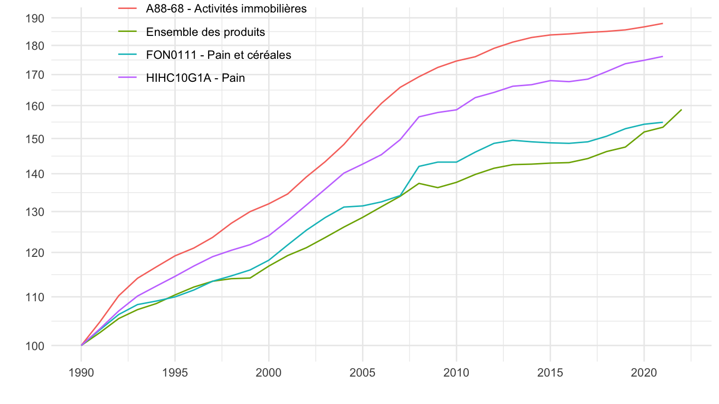

Price Deflator

A10

Code

`CNA-2014-CONSO-MEN` |>
  filter(grepl("A10", CNA_PRODUIT),
         TIME_PERIOD %in% c("2019", "1959"),
         UNIT_MEASURE == "SO") |>
  
  arrange(CNA_PRODUIT) |>
  select(CNA_PRODUIT, CNA_PRODUIT, TIME_PERIOD, OBS_VALUE) |>
  spread(TIME_PERIOD, OBS_VALUE) |>
  mutate(`Avg growth` = round(100*((`2019`/`1959`)^(1/60)-1), 1)) |>
  arrange(-`Avg growth`) |>
  print_table_conditional()

CNA_PRODUIT	1959	2019	Avg growth
A10-FZ	4.0	108.7	5.7
A10-GI	4.3	107.9	5.5
A10-RU	4.1	102.1	5.5
A10-LZ	4.4	101.5	5.4
A10-OQ	6.4	103.9	4.8
A10-MN	8.7	100.7	4.2
A10-KZ	9.8	109.5	4.1
A10-AZ	11.6	120.9	4.0
A10-BE	14.9	102.0	3.3
A10-JZ	22.1	97.8	2.5

A17

Code

`CNA-2014-CONSO-MEN` |>
  filter(grepl("A17", CNA_PRODUIT),
         TIME_PERIOD %in% c("2019", "1959"),
         UNIT_MEASURE == "SO") |>
  
  arrange(CNA_PRODUIT) |>
  select(CNA_PRODUIT, CNA_PRODUIT, TIME_PERIOD, OBS_VALUE) |>
  spread(TIME_PERIOD, OBS_VALUE) |>
  mutate(`Avg growth` = round(100*((`2019`/`1959`)^(1/60)-1), 1)) |>
  arrange(-`Avg growth`) |>
  print_table_conditional()

CNA_PRODUIT	1959	2019	Avg growth
A17-GZ	1.6	109.6	7.3
A17-FZ	4.0	108.7	5.7
A17-IZ	4.3	108.6	5.5
A17-RU	4.1	102.1	5.5
A17-LZ	4.4	101.5	5.4
A17-C2	6.6	107.1	4.8
A17-HZ	6.5	105.9	4.8
A17-OQ	6.4	103.9	4.8
A17-MN	8.7	100.7	4.2
A17-KZ	9.8	109.5	4.1
A17-AZ	11.6	120.9	4.0
A17-C1	10.7	106.4	3.9
A17-DE	11.3	110.6	3.9
A17-C4	13.6	103.1	3.4
A17-C5	15.9	97.4	3.1
A17-JZ	22.1	97.8	2.5
A17-C3	315.2	83.5	-2.2

A38

Code

`CNA-2014-CONSO-MEN` |>
  filter(grepl("A38", CNA_PRODUIT),
         TIME_PERIOD %in% c("2019", "1959"),
         UNIT_MEASURE == "SO") |>
  
  arrange(CNA_PRODUIT) |>
  select(CNA_PRODUIT, CNA_PRODUIT, TIME_PERIOD, OBS_VALUE) |>
  spread(TIME_PERIOD, OBS_VALUE) |>
  mutate(`Avg growth` = round(100*((`2019`/`1959`)^(1/60)-1), 1)) |>
  arrange(-`Avg growth`) |>
  print_table_conditional()

A88

Code

`CNA-2014-CONSO-MEN` |>
  filter(grepl("A88", CNA_PRODUIT),
         TIME_PERIOD %in% c("2019", "1959"),
         UNIT_MEASURE == "SO") |>
  
  arrange(CNA_PRODUIT) |>
  select(CNA_PRODUIT, CNA_PRODUIT, TIME_PERIOD, OBS_VALUE) |>
  spread(TIME_PERIOD, OBS_VALUE) |>
  mutate(`Avg growth` = round(100*((`2019`/`1959`)^(1/60)-1), 1)) |>
  arrange(-`Avg growth`) |>
  print_table_conditional()

DUR

Code

`CNA-2014-CONSO-MEN` |>
  filter(grepl("DUR", CNA_PRODUIT),
         TIME_PERIOD %in% c("2019", "1959"),
         UNIT_MEASURE == "SO") |>
  
  arrange(CNA_PRODUIT) |>
  select(CNA_PRODUIT, CNA_PRODUIT, TIME_PERIOD, OBS_VALUE) |>
  spread(TIME_PERIOD, OBS_VALUE) |>
  mutate(`Avg growth` = round(100*((`2019`/`1959`)^(1/60)-1), 1)) |>
  arrange(-`Avg growth`) |>
  print_table_conditional()

CNA_PRODUIT	1959	2019	Avg growth
DUR44	4.3	108.6	5.5
DUR41	4.4	101.5	5.4
DUR45	5.2	103.6	5.1
DUR46	5.7	106.2	5.0
DUR4	6.0	103.8	4.9
DUR32	8.7	109.2	4.3
DUR42	8.2	101.2	4.3
DURTOTAL	9.5	103.4	4.1
DUR3	11.6	105.8	3.8
DUR31	11.9	106.7	3.7
DUR5	11.8	103.9	3.7
DUR12	12.7	99.5	3.5
DUR21	13.4	99.2	3.4
DUR33	15.2	101.8	3.2
DUR11	15.9	101.7	3.1
DUR2	15.7	98.6	3.1
DUR43	16.7	101.3	3.1
DUR22	20.1	97.9	2.7
DUR1	33.6	96.3	1.8
DUR14	74.5	91.6	0.3
DUR13	85.3	91.1	0.1

FON

Code

`CNA-2014-CONSO-MEN` |>
  filter(grepl("FON", CNA_PRODUIT),
         TIME_PERIOD %in% c("2019", "1959"),
         UNIT_MEASURE == "SO") |>
  
  arrange(CNA_PRODUIT) |>
  select(CNA_PRODUIT, CNA_PRODUIT, TIME_PERIOD, OBS_VALUE) |>
  spread(TIME_PERIOD, OBS_VALUE) |>
  mutate(`Avg growth` = round(100*((`2019`/`1959`)^(1/60)-1), 1)) |>
  arrange(-`Avg growth`) |>
  print_table_conditional()

GG

Code

`CNA-2014-CONSO-MEN` |>
  filter(grepl("GG", CNA_PRODUIT),
         TIME_PERIOD %in% c("2019", "1959"),
         UNIT_MEASURE == "SO") |>
  
  arrange(CNA_PRODUIT) |>
  select(CNA_PRODUIT, CNA_PRODUIT, TIME_PERIOD, OBS_VALUE) |>
  spread(TIME_PERIOD, OBS_VALUE) |>
  mutate(`Avg growth` = round(100*((`2019`/`1959`)^(1/60)-1), 1)) |>
  arrange(-`Avg growth`) |>
  print_table_conditional()

Related Data

Données sur l’inflation en France

source	dataset	Title	Updated
insee	ILC-ILAT-ICC	Indices pour la révision d’un bail commercial ou professionnel - ILC-ILAT-ICC	2026-08-16
insee	INDICES_LOYERS	Indices des loyers d'habitation (ILH) - INDICES_LOYERS	2026-08-16
insee	IPC-1970-1980	Indice des prix à la consommation - Base 1970, 1980 - IPC-1970-1980	2026-08-16
insee	IPC-1990	Indices des prix à la consommation - Base 1990 - IPC-1990	2026-08-16
insee	IPC-2015	Indice des prix à la consommation - Base 2015 - IPC-2015	2026-08-17
insee	IPC-PM-2015	Prix moyens de vente de détail - IPC-PM-2015	2026-08-16
insee	IPCH-2015	Indices des prix à la consommation harmonisés - IPCH-2015	2026-08-16
insee	IPCH-IPC-2015-ensemble	Indices des prix à la consommation harmonisés - IPCH-IPC-2015-ensemble	2026-08-02
insee	IPGD-2015	Indice des prix dans la grande distribution - IPGD-2015	2026-08-13
insee	IPLA-IPLNA-2015	Indices des prix des logements neufs et Indices Notaires-Insee des prix des logements anciens - IPLA-IPLNA-2015	2026-08-16
insee	IPPI-2015	Indices de prix de production et d'importation dans l'industrie - IPPI-2015	2026-08-17
insee	IRL	Indice pour la révision d’un loyer d’habitation - IRL	2026-09-03
insee	SERIES_LOYERS	Variation des loyers - SERIES_LOYERS	2026-08-16
insee	T_CONSO_EFF_FONCTION	Consommation effective des ménages par fonction - T_CONSO_EFF_FONCTION	2026-09-02
insee	bdf2017	Budget de famille 2017 - bdf2017	2026-08-13
insee	echantillon-agglomerations-IPC-2024	Échantillon d’agglomérations enquêtées de l’IPC en 2024 - echantillon-agglomerations-IPC-2024	2026-08-02
insee	echantillon-agglomerations-IPC-2025	Échantillon d’agglomérations enquêtées de l’IPC en 2025 - echantillon-agglomerations-IPC-2025	2026-08-02
insee	liste-varietes-IPC-2024	Liste des variétés pour la mesure de l'IPC en 2024 - liste-varietes-IPC-2024	2026-08-02
insee	liste-varietes-IPC-2025	Liste des variétés pour la mesure de l'IPC en 2025 - liste-varietes-IPC-2025	2026-08-02
insee	ponderations-elementaires-IPC-2024	Pondérations élémentaires 2024 intervenant dans le calcul de l’IPC - ponderations-elementaires-IPC-2024	2026-08-02
insee	ponderations-elementaires-IPC-2025	Pondérations élémentaires 2025 intervenant dans le calcul de l’IPC - ponderations-elementaires-IPC-2025	2026-08-02
insee	table_conso_moyenne_par_categorie_menages	Montants de consommation selon différentes catégories de ménages - table_conso_moyenne_par_categorie_menages	2026-08-02
insee	table_poste_au_sein_sous_classe_ecoicopv2_france_entiere_	Ventilation de chaque sous-classe (niveau 4 de la COICOP v2) en postes et leurs pondérations - table_poste_au_sein_sous_classe_ecoicopv2_france_entiere_	2026-08-02
insee	tranches_unitesurbaines	Poids de chaque tranche d’unités urbaines dans la consommation - tranches_unitesurbaines	2026-08-02

Data on inflation

source	dataset	Title	Updated
bis	CPI	Consumer Price Index - CPI	2026-08-31
ecb	CES	Consumer Expectations Survey - CES	2026-08-31
eurostat	nama_10_co3_p3	Final consumption expenditure of households by consumption purpose (COICOP 3 digit) - nama_10_co3_p3	2026-08-30
eurostat	prc_hicp_cow	HICP - country weights - prc_hicp_cow	2026-07-15
eurostat	prc_hicp_ctrb	Contributions to euro area annual inflation (in percentage points) - prc_hicp_ctrb	2026-07-14
eurostat	prc_hicp_inw	HICP - item weights - prc_hicp_inw	2026-07-15
eurostat	prc_hicp_manr	HICP (2015 = 100) - monthly data (annual rate of change) - prc_hicp_manr	2026-08-07
eurostat	prc_hicp_midx	HICP (2015 = 100) - monthly data (index) - prc_hicp_midx	2026-08-07
eurostat	prc_hicp_mmor	HICP (2015 = 100) - monthly data (monthly rate of change) - prc_hicp_mmor	2026-08-13
eurostat	prc_ppp_ind	Purchasing power parities (PPPs), price level indices and real expenditures for ESA 2010 aggregates - prc_ppp_ind	2026-07-27
eurostat	sts_inpp_m	Producer prices in industry, total - monthly data - sts_inpp_m	2026-08-30
eurostat	sts_inppd_m	Producer prices in industry, domestic market - monthly data - sts_inppd_m	2026-08-30
eurostat	sts_inppnd_m	Producer prices in industry, non domestic market - monthly data - sts_inppnd_m	2026-08-30
fred	cpi	Consumer Price Index - cpi	2026-09-01
fred	inflation	Inflation - inflation	2026-09-01
imf	CPI	Consumer Price Index (CPI) 2026 February - CPI_2026_FEB_VINTAGE - CPI	2026-07-25
oecd	MEI_PRICES_PPI	Producer Prices - MEI_PRICES_PPI	2026-08-02
oecd	PPP2017	2017 PPP Benchmark results - PPP2017	2026-08-02
oecd	PRICES_CPI	Consumer price indices (CPIs) - PRICES_CPI	2026-08-02
wdi	FP.CPI.TOTL.ZG	Inflation, consumer prices (annual %) - FP.CPI.TOTL.ZG	2026-09-01
wdi	NY.GDP.DEFL.KD.ZG	Inflation, GDP deflator (annual %) - NY.GDP.DEFL.KD.ZG	2026-09-01