Job Openings and Labor Turnover Survey - JT
Data - BLS
Info
Data on employment
| source | dataset | .html | .RData |
|---|---|---|---|
| bls | jt | 2024-11-12 | NA |
| bls | la | 2024-11-12 | NA |
| bls | ln | 2024-11-12 | NA |
| eurostat | nama_10_a10_e | 2025-08-24 | 2025-08-24 |
| eurostat | nama_10_a64_e | 2025-08-24 | 2025-08-24 |
| eurostat | namq_10_a10_e | 2025-05-24 | 2025-08-24 |
| eurostat | une_rt_m | 2025-08-24 | 2025-08-24 |
| oecd | ALFS_EMP | 2024-04-16 | 2025-05-24 |
| oecd | EPL_T | 2025-08-20 | 2023-12-10 |
| oecd | LFS_SEXAGE_I_R | 2024-09-15 | 2024-04-15 |
| oecd | STLABOUR | 2025-01-17 | 2025-01-17 |
LAST_DOWNLOAD
| LAST_DOWNLOAD |
|---|
| 2024-11-12 |
LAST_COMPILE
| LAST_COMPILE |
|---|
| 2025-08-24 |
Last
| date | Nobs |
|---|---|
| 2024-09-01 | 913 |
jt.industry
Code
jt.data.1.AllItems %>%
  left_join(jt.series, by = "series_id") %>%
  left_join(jt.industry, by = "industry_code") %>%
  group_by(industry_code, industry_text) %>%
  summarise(Nobs = n()) %>%
print_table_conditional| industry_code | industry_text | Nobs |
|---|---|---|
| 0 | Total nonfarm | 352951 |
| 100000 | Total private | 48324 |
| 110099 | Mining and logging | 7140 |
| 230000 | Construction | 7140 |
| 300000 | Manufacturing | 7140 |
| 320000 | Durable goods manufacturing | 7140 |
| 340000 | Nondurable goods manufacturing | 7140 |
| 400000 | Trade, transportation, and utilities | 7140 |
| 420000 | Wholesale trade | 7140 |
| 440000 | Retail trade | 7140 |
| 480099 | Transportation, warehousing, and utilities | 7140 |
| 510000 | Information | 7140 |
| 510099 | Financial activities | 7140 |
| 520000 | Finance and insurance | 7140 |
| 530000 | Real estate and rental and leasing | 7140 |
| 540099 | Professional and business services | 7140 |
| 600000 | Education and health services | 7140 |
| 610000 | Educational services | 7140 |
| 620000 | Health care and social assistance | 7140 |
| 700000 | Leisure and hospitality | 7140 |
| 710000 | Arts, entertainment, and recreation | 7140 |
| 720000 | Accommodation and food services | 7140 |
| 810000 | Other services | 7140 |
| 900000 | Government | 7140 |
| 910000 | Federal | 7140 |
| 920000 | State and local | 7140 |
| 923000 | State and local government education | 7140 |
| 929000 | State and local government, excluding education | 7140 |
jt.dataelement
Code
jt.data.1.AllItems %>%
  left_join(jt.series, by = "series_id") %>%
  left_join(jt.dataelement, by = "dataelement_code") %>%
  group_by(dataelement_code, dataelement_text) %>%
  summarise(Nobs = n()) %>%
print_table_conditional| dataelement_code | dataelement_text | Nobs |
|---|---|---|
| HI | Hires | 105430 |
| JO | Job openings | 105430 |
| LD | Layoffs and discharges | 105430 |
| OS | Other separations | 44944 |
| QU | Quits | 105430 |
| TS | Total separations | 105430 |
| UO | Unemployed persons per job opening ratio | 14821 |
jt.ratelevel
Code
jt.data.1.AllItems %>%
  left_join(jt.series, by = "series_id") %>%
  left_join(jt.ratelevel, by = "ratelevel_code") %>%
  group_by(ratelevel_code, ratelevel_text) %>%
  summarise(Nobs = n()) %>%
print_table_conditional| ratelevel_code | ratelevel_text | Nobs |
|---|---|---|
| L | Level - In Thousands | 286047 |
| R | Rate | 300868 |
jt.region
Code
jt.region %>%
{if (is_html_output()) print_table(.) else .}| region_code | region_text | display_level | selectable | sort_sequence |
|---|---|---|---|---|
| 00 | Total US | 0 | T | 1 |
| MW | Midwest (Only available for Total Nonfarm) | 1 | T | 4 |
| NE | Northeast (Only available for Total Nonfarm) | 1 | T | 2 |
| SO | South (Only available for Total Nonfarm) | 1 | T | 3 |
| WE | West (Only available for Total Nonfarm) | 1 | T | 5 |
jt.seasonal
Code
jt.data.1.AllItems %>%
  left_join(jt.series, by = "series_id") %>%
  left_join(jt.seasonal, by = c("seasonal" = "seasonal_code")) %>%
  group_by(seasonal, seasonal_text) %>%
  summarise(Nobs = n()) %>%
print_table_conditional| seasonal | seasonal_text | Nobs |
|---|---|---|
| S | Seasonally Adjusted | 290587 |
| U | Not Seasonally Adjusted | 296328 |
Monthly Job Openings, Layoffs and Quits, in Thousands
All
Code
jt.data.1.AllItems %>%
  filter(series_id %in% c("JTS000000000000000LDL",
                          "JTS000000000000000QUL",
                          "JTS000000000000000JOL")) %>%
  left_join(jt.series, by = "series_id") %>%
  left_join(jt.dataelement, by = "dataelement_code") %>%
  month_to_date %>%
  ggplot(.) +
  geom_line(aes(x = date, y = value, color = dataelement_text)) +
  theme_minimal() +
  theme(legend.title = element_blank(),
        legend.position = c(0.6, 0.85)) +
  scale_x_date(breaks = as.Date(paste0(seq(1930, 2100, 2), "-01-01")),
               labels = date_format("%Y")) +
  geom_rect(data = nber_recessions %>%
              filter(Peak > as.Date("1996-01-01")),
            aes(xmin = Peak, xmax = Trough, ymin = -Inf, ymax = +Inf),
            fill = 'grey', alpha = 0.5) +
  scale_y_continuous(breaks = 1000*seq(0, 20, 1),
                     labels = dollar_format(suffix = "K", prefix = "")) +
  xlab("") + ylab("Monthly Levels ('000s)")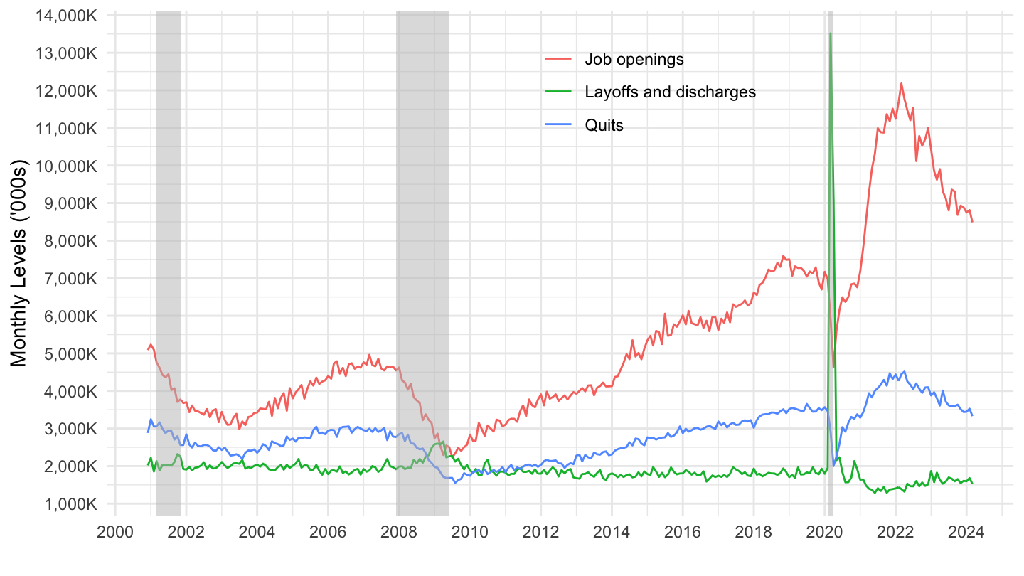
Monthly Hires and Separations, in Thousands
All
Code
jt.data.1.AllItems %>%
  filter(series_id %in% c("JTS000000000000000HIL",
                          "JTS000000000000000TSL")) %>%
  left_join(jt.series, by = "series_id") %>%
  left_join(jt.dataelement, by = "dataelement_code") %>%
  month_to_date %>%
  ggplot(.) +
  geom_line(aes(x = date, y = value, color = dataelement_text)) +
  theme_minimal() +
  theme(legend.title = element_blank(),
        legend.position = c(0.6, 0.85)) +
  scale_x_date(breaks = as.Date(paste0(seq(1930, 2100, 2), "-01-01")),
               labels = date_format("%Y")) +
  geom_rect(data = nber_recessions %>%
              filter(Peak > as.Date("1996-01-01")),
            aes(xmin = Peak, xmax = Trough, ymin = -Inf, ymax = +Inf),
            fill = 'grey', alpha = 0.5) +
  scale_y_continuous(breaks = 1000*seq(0, 20, 1),
                     labels = dollar_format(suffix = "K", prefix = "")) +
  xlab("") + ylab("Monthly Levels ('000s)")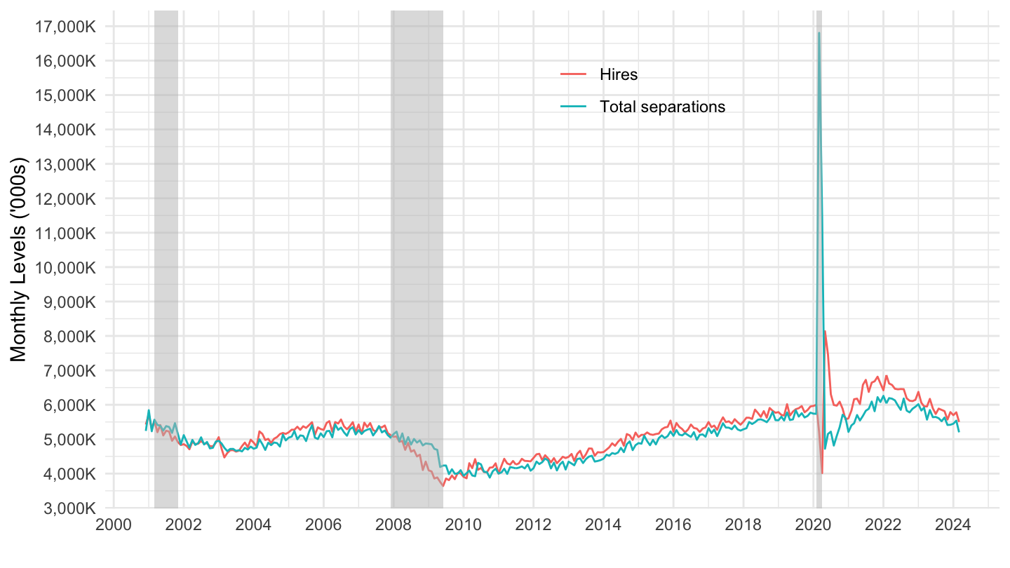
Limits
Code
jt.data.1.AllItems %>%
  filter(series_id %in% c("JTS000000000000000HIL",
                          "JTS000000000000000TSL")) %>%
  left_join(jt.series, by = "series_id") %>%
  left_join(jt.dataelement, by = "dataelement_code") %>%
  month_to_date %>%
  ggplot(.) +
  geom_line(aes(x = date, y = value, color = dataelement_text)) +
  theme_minimal() +
  theme(legend.title = element_blank(),
        legend.position = c(0.6, 0.85)) +
  scale_x_date(breaks = as.Date(paste0(seq(1930, 2100, 2), "-01-01")),
               labels = date_format("%Y")) +
  geom_rect(data = nber_recessions %>%
              filter(Peak > as.Date("1996-01-01")),
            aes(xmin = Peak, xmax = Trough, ymin = -Inf, ymax = +Inf),
            fill = 'grey', alpha = 0.5) +
  scale_y_continuous(breaks = 1000*seq(0, 20, 1),
                     labels = dollar_format(suffix = "K", prefix = ""),
                     limits = c(3000, 9000)) +
  xlab("") + ylab("Monthly Levels ('000s)")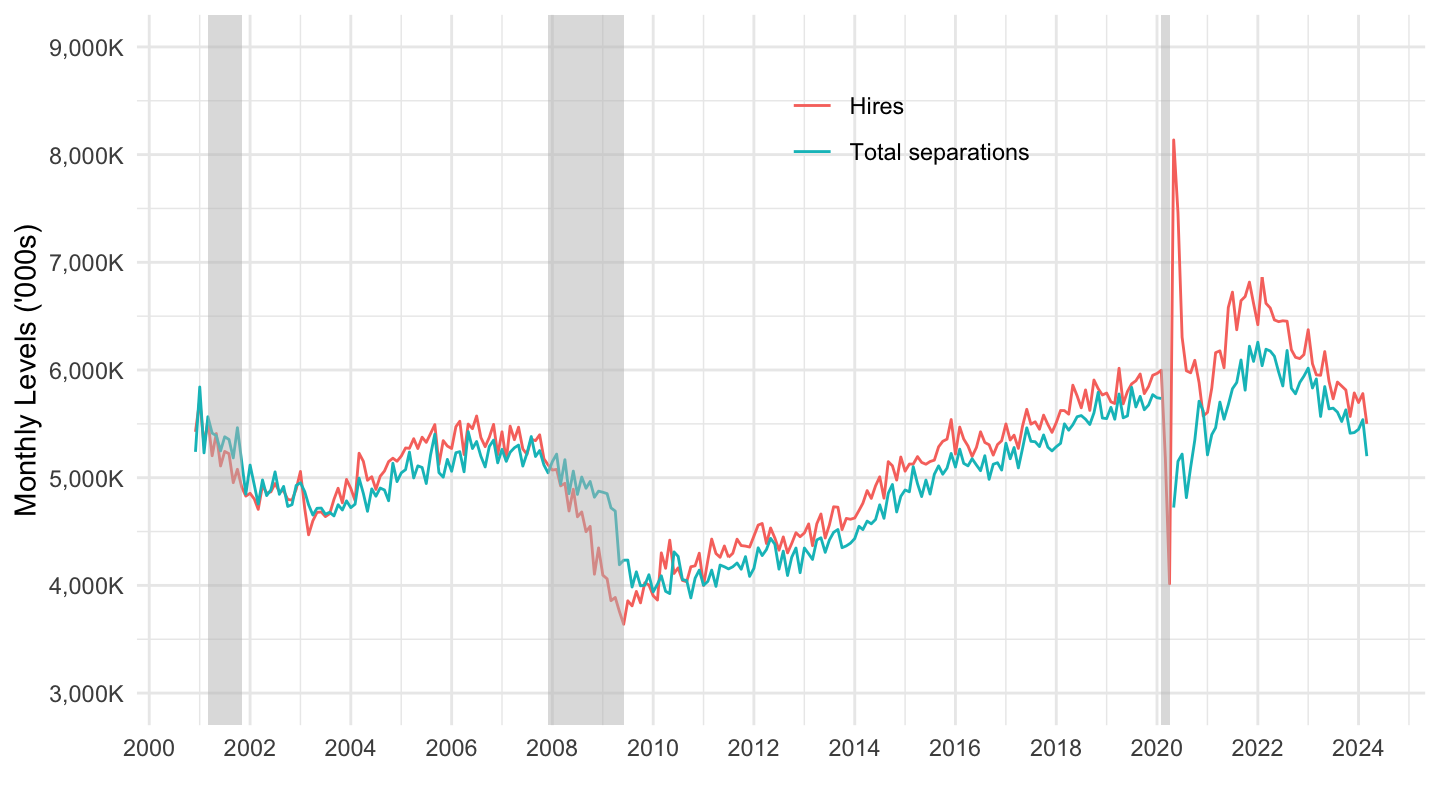
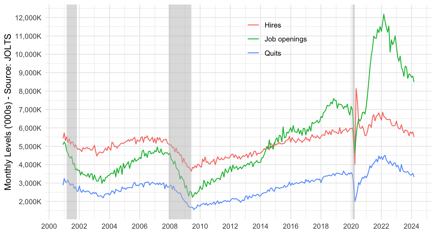
Monthly Hires, quits, Openings
All
Code
jt.data.1.AllItems %>%
  filter(series_id %in% c("JTS000000000000000HIL",
                          "JTS000000000000000JOL",
                          "JTS000000000000000QUL")) %>%
  left_join(jt.series, by = "series_id") %>%
  left_join(jt.dataelement, by = "dataelement_code") %>%
  month_to_date %>%
  ggplot(.) +
  geom_line(aes(x = date, y = value, color = dataelement_text)) +
  theme_minimal() +
  theme(legend.title = element_blank(),
        legend.position = c(0.6, 0.85)) +
  scale_x_date(breaks = as.Date(paste0(seq(1930, 2100, 2), "-01-01")),
               labels = date_format("%Y")) +
  geom_rect(data = nber_recessions %>%
              filter(Peak > as.Date("1996-01-01")),
            aes(xmin = Peak, xmax = Trough, ymin = -Inf, ymax = +Inf),
            fill = 'grey', alpha = 0.5) +
  scale_y_continuous(breaks = 1000*seq(0, 20, 1),
                     labels = dollar_format(suffix = "K", prefix = "")) +
  xlab("") + ylab("Monthly Levels ('000s) - Source: JOLTS")