| source | dataset | Title | .html | .rData |
|---|---|---|---|---|
| oecd | LFS_SEXAGE_I_R | LFS by sex and age - indicators | 2026-07-23 | 2024-04-15 |
LFS by sex and age - indicators
Data - OECD
Info
Data on employment
Code
load_data("employment.RData")
employment %>%
  arrange(-(dataset == "LFS_SEXAGE_I_R")) %>%
source_dataset_file_updates()| source | dataset | Title | .html | .rData |
|---|---|---|---|---|
| oecd | LFS_SEXAGE_I_R | LFS by sex and age - indicators | 2026-07-23 | 2024-04-15 |
| bls | jt | NA | NA | NA |
| bls | la | NA | NA | NA |
| bls | ln | NA | NA | NA |
| eurostat | nama_10_a10_e | Employment by A*10 industry breakdowns | 2026-07-23 | 2026-07-23 |
| eurostat | nama_10_a64_e | National accounts employment data by industry (up to NACE A*64) | 2026-07-23 | 2026-07-23 |
| eurostat | namq_10_a10_e | Employment A*10 industry breakdowns | 2026-07-23 | 2026-07-23 |
| eurostat | une_rt_m | Unemployment by sex and age – monthly data | 2026-07-23 | 2026-07-23 |
| oecd | ALFS_EMP | Employment by activities and status (ALFS) | 2024-04-16 | 2025-05-24 |
| oecd | EPL_T | Strictness of employment protection – temporary contracts | 2026-07-23 | 2023-12-10 |
| oecd | STLABOUR | Short-Term Labour Market Statistics | 2026-07-23 | 2025-01-17 |
Données sur l’emploi
| source | dataset | Title | .html | .rData |
|---|---|---|---|---|
| insee | CHOMAGE-TRIM-NATIONAL | Chômage, taux de chômage par sexe et âge (sens BIT) (1975-) | 2026-07-23 | 2026-07-23 |
| insee | CNA-2014-EMPLOI | Emploi intérieur, durée effective travaillée et productivité horaire | 2026-07-23 | 2026-07-22 |
| insee | DEMANDES-EMPLOIS-NATIONALES | Demandeurs d'emploi inscrits à Pôle Emploi | 2026-07-23 | 2026-07-23 |
| insee | EMPLOI-BIT-TRIM | Emploi, activité, sous-emploi par secteur d’activité (sens BIT) | 2026-07-23 | 2026-07-23 |
| insee | EMPLOI-SALARIE-TRIM-NATIONAL | Estimations d'emploi salarié par secteur d'activité | 2026-07-23 | 2026-07-23 |
| insee | TAUX-CHOMAGE | Taux de chômage localisé | 2026-07-23 | 2026-07-23 |
| insee | TCRED-EMPLOI-SALARIE-TRIM | Estimations d'emploi salarié par secteur d'activité et par département | 2026-07-23 | 2026-07-23 |
LAST_COMPILE
| LAST_COMPILE |
|---|
| 2026-07-24 |
Last
| obsTime | Nobs |
|---|---|
| 2022 | 12100 |
SEX
Code
LFS_SEXAGE_I_R %>%
  left_join(LFS_SEXAGE_I_R_var$SEX, by = "SEX") %>%
  group_by(SEX, Sex) %>%
  summarise(Nobs = n()) %>%
  arrange(-Nobs) %>%
print_table_conditional()| SEX | Sex | Nobs |
|---|---|---|
| MW | All persons | 153275 |
| MEN | Men | 152299 |
| WOMEN | Women | 150636 |
AGE
Code
LFS_SEXAGE_I_R %>%
  left_join(LFS_SEXAGE_I_R_var$AGE, by = "AGE") %>%
  group_by(AGE, Age) %>%
  summarise(Nobs = n()) %>%
  arrange(-Nobs) %>%
  print_table_conditional()
SERIES
Code
LFS_SEXAGE_I_R %>%
  left_join(LFS_SEXAGE_I_R_var$SERIES, by = "SERIES") %>%
  group_by(SERIES, Series) %>%
  summarise(Nobs = n()) %>%
  arrange(-Nobs) %>%
print_table_conditional()| SERIES | Series | Nobs |
|---|---|---|
| LFPR | Labour force participation rate | 156928 |
| EPR | Employment/population ratio | 156551 |
| UR | Unemployment rate | 142731 |
FREQUENCY
Code
LFS_SEXAGE_I_R %>%
  left_join(LFS_SEXAGE_I_R_var$FREQUENCY, by = "FREQUENCY") %>%
  group_by(FREQUENCY, Frequency) %>%
  summarise(Nobs = n()) %>%
  arrange(-Nobs) %>%
print_table_conditional()| FREQUENCY | Frequency | Nobs |
|---|---|---|
| A | Annual | 456210 |
COUNTRY
Code
LFS_SEXAGE_I_R %>%
  left_join(LFS_SEXAGE_I_R_var$COUNTRY, by = "COUNTRY") %>%
  group_by(COUNTRY, Country) %>%
  summarise(Nobs = n()) %>%
  arrange(-Nobs) %>%
  mutate(Flag = gsub(" ", "-", str_to_lower(gsub(" ", "-", Country))),
         Flag = paste0('<img src="../../icon/flag/round/vsmall/', Flag, '.png" alt="Flag">')) %>%
  select(Flag, everything()) %>%
  {if (is_html_output()) datatable(., filter = 'top', rownames = F, escape = F) else .}
obsTime
Code
LFS_SEXAGE_I_R %>%
  group_by(obsTime) %>%
  summarise(Nobs = n()) %>%
  arrange(desc(obsTime)) %>%
  print_table_conditional()
Denmark, France, United States
25-54
Code
LFS_SEXAGE_I_R %>%
  filter(SERIES == "EPR",
         AGE == "2554",
         SEX == "MW",
         COUNTRY %in% c("DNK", "USA", "FRA")) %>%
  year_to_date %>%
  left_join(LFS_SEXAGE_I_R_var$COUNTRY, by = "COUNTRY") %>%
  select(Location = Country, date, obsValue) %>%
  arrange(Location, date) %>%
  mutate(obsValue = obsValue/100) %>%
  left_join(colors, by = c("Location" = "country")) %>%
  ggplot(.) + geom_line(aes(x = date, y = obsValue, color = color, linetype = color)) +
  scale_color_identity() +
  theme_minimal() + xlab("") + ylab("Employment / Population, 25-54") +
  add_3flags +
  scale_x_date(breaks = seq(1960, 2100, 5) %>% paste0("-01-01") %>% as.Date,
               labels = date_format("%Y")) +
  theme(legend.position = "none") +
  scale_y_continuous(breaks = 0.01*seq(0, 200, 2),
                     labels = scales::percent_format(accuracy = 1))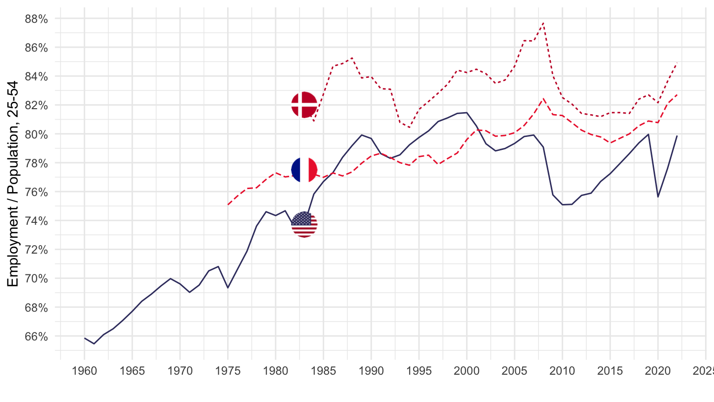
25-64
Code
LFS_SEXAGE_I_R %>%
  filter(SERIES == "EPR",
         AGE == "2564",
         SEX == "MW",
         COUNTRY %in% c("DNK", "USA", "FRA")) %>%
  year_to_date %>%
  left_join(LFS_SEXAGE_I_R_var$COUNTRY, by = "COUNTRY") %>%
  select(Location = Country, date, obsValue) %>%
  arrange(Location, date) %>%
  mutate(obsValue = obsValue/100) %>%
  left_join(colors, by = c("Location" = "country")) %>%
  ggplot(.) + geom_line(aes(x = date, y = obsValue, color = color, linetype = color)) +
  scale_color_identity() +
  theme_minimal() + xlab("") + ylab("Employment / Population, 25-64") +
  add_3flags +
  scale_x_date(breaks = seq(1960, 2100, 5) %>% paste0("-01-01") %>% as.Date,
               labels = date_format("%Y")) +
  theme(legend.position = "none") +
  scale_y_continuous(breaks = 0.01*seq(0, 200, 2),
                     labels = scales::percent_format(accuracy = 1))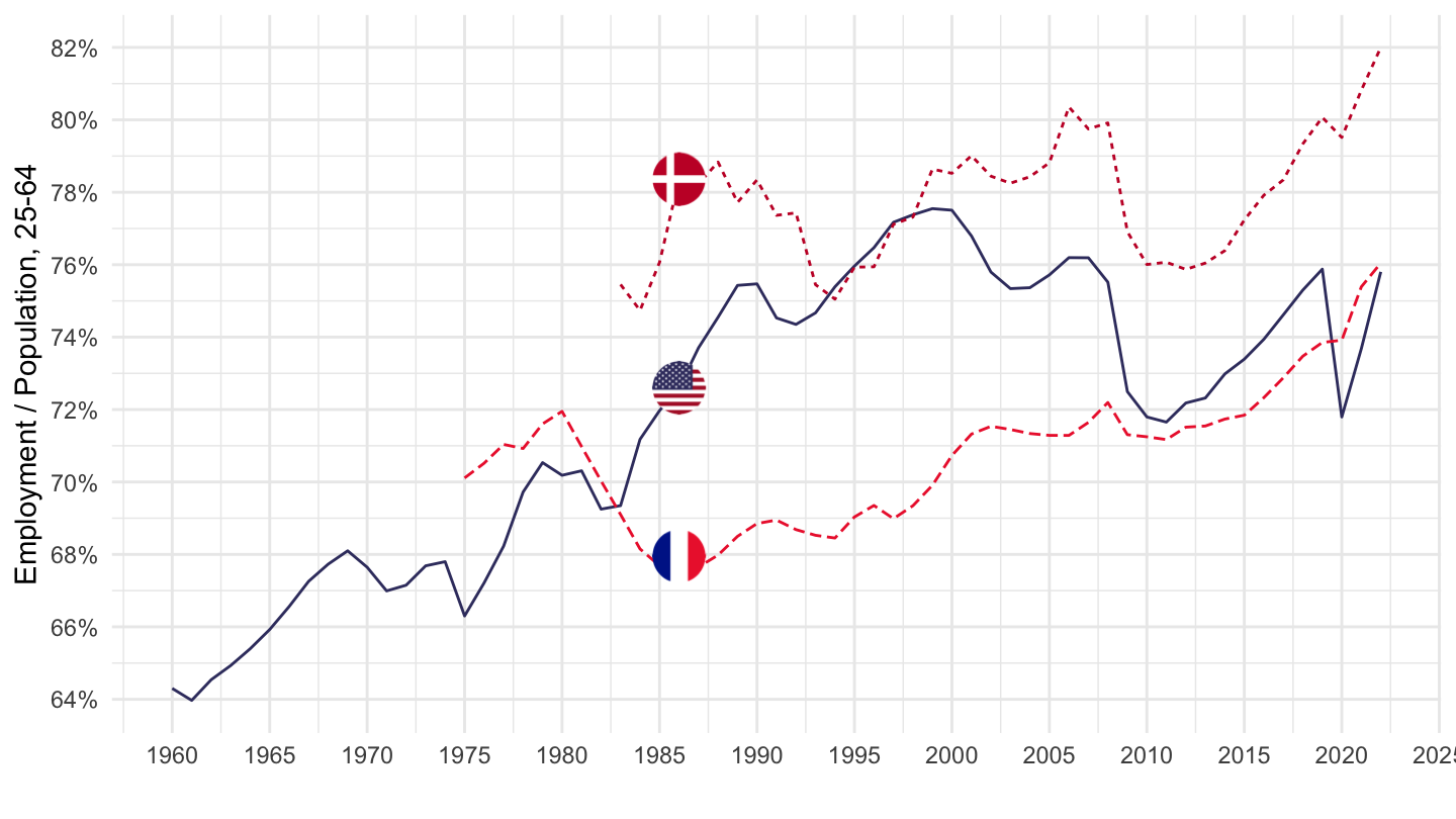
20-64
Code
LFS_SEXAGE_I_R %>%
  filter(SERIES == "EPR",
         AGE == "2064",
         SEX == "MW",
         COUNTRY %in% c("DNK", "USA", "FRA")) %>%
  year_to_date %>%
  left_join(LFS_SEXAGE_I_R_var$COUNTRY, by = "COUNTRY") %>%
  select(Location = Country, date, obsValue) %>%
  arrange(Location, date) %>%
  mutate(obsValue = obsValue/100) %>%
  left_join(colors, by = c("Location" = "country")) %>%
  ggplot(.) + geom_line(aes(x = date, y = obsValue, color = color, linetype = color)) +
  scale_color_identity() +
  theme_minimal() + xlab("") + ylab("Employment / Population, 20-64") +
  add_3flags +
  scale_x_date(breaks = seq(1960, 2100, 5) %>% paste0("-01-01") %>% as.Date,
               labels = date_format("%Y")) +
  theme(legend.position = "none") +
  scale_y_continuous(breaks = 0.01*seq(0, 200, 2),
                     labels = scales::percent_format(accuracy = 1))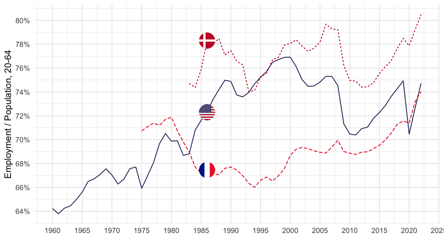
Unemployment Rate
Code
LFS_SEXAGE_I_R %>%
  filter(SERIES == "UR",
         AGE == "1564",
         SEX == "MW",
         COUNTRY %in% c("DNK", "USA", "FRA")) %>%
  year_to_date %>%
  left_join(LFS_SEXAGE_I_R_var$COUNTRY, by = "COUNTRY") %>%
  select(Location = Country, date, obsValue) %>%
  arrange(Location, date) %>%
  mutate(obsValue = obsValue/100) %>%
  left_join(colors, by = c("Location" = "country")) %>%
  ggplot(.) + geom_line(aes(x = date, y = obsValue, color = color, linetype = color)) +
  scale_color_identity() +
  theme_minimal() + xlab("") + ylab("Unemployment Rate") +
  add_3flags +
  scale_x_date(breaks = seq(1960, 2100, 5) %>% paste0("-01-01") %>% as.Date,
               labels = date_format("%Y")) +
  theme(legend.position = "none") +
  scale_y_continuous(breaks = 0.01*seq(0, 200, 1),
                     labels = scales::percent_format(accuracy = 1))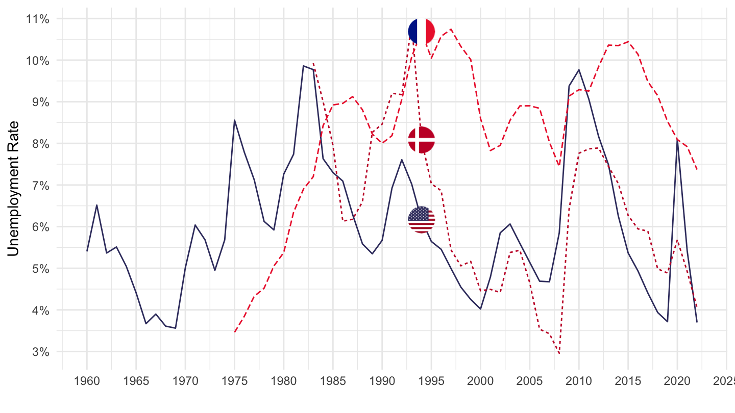
Germany, France, Italy, United States, Spain
All
Code
LFS_SEXAGE_I_R %>%
  filter(SERIES == "EPR",
         AGE == "900000",
         SEX == "MW",
         COUNTRY %in% c("ITA", "DEU", "FRA", "ESP", "USA")) %>%
  year_to_date %>%
  left_join(LFS_SEXAGE_I_R_var$COUNTRY, by = "COUNTRY") %>%
  select(COUNTRY, Location = Country, date, obsValue) %>%
  left_join(colors, by = c("Location" = "country")) %>%
  mutate(obsValue = obsValue/100) %>%
  mutate(color = ifelse(COUNTRY == "USA", color2, color)) %>%
  ggplot(.) + geom_line(aes(x = date, y = obsValue, color = color)) +
  scale_color_identity() +
  theme_minimal() + xlab("") + ylab("Employment / Population, Total") +
  add_5flags +
  scale_x_date(breaks = seq(1960, 2100, 5) %>% paste0("-01-01") %>% as.Date,
               labels = date_format("%Y")) +
  theme(legend.position = "none") +
  scale_y_continuous(breaks = 0.01*seq(0, 200, 5),
                     labels = scales::percent_format(accuracy = 1))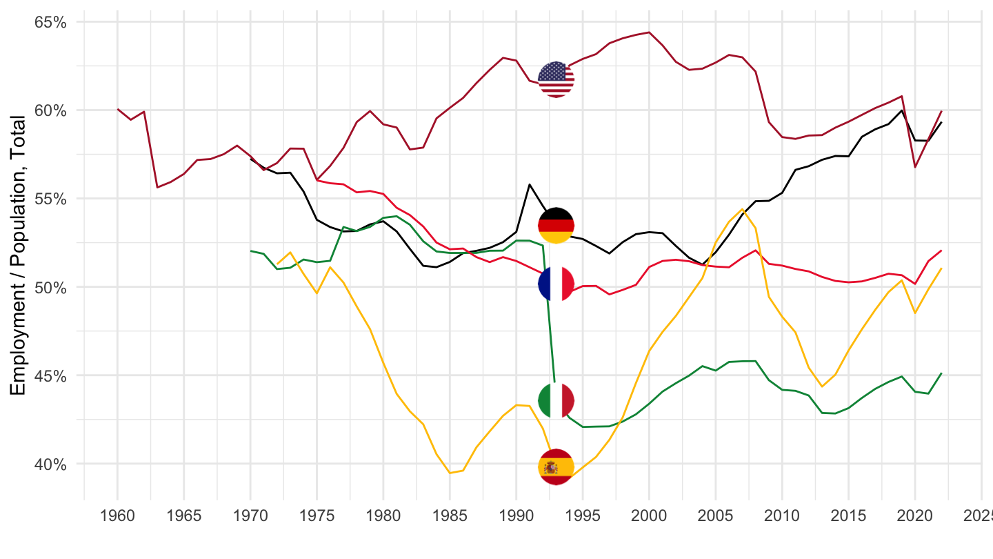
1975-
Code
LFS_SEXAGE_I_R %>%
  filter(SERIES == "EPR",
         AGE == "900000",
         SEX == "MW",
         COUNTRY %in% c("ITA", "DEU", "FRA", "ESP", "USA")) %>%
  year_to_date %>%
  filter(date >= as.Date("1975-01-01")) %>%
  left_join(LFS_SEXAGE_I_R_var$COUNTRY, by = "COUNTRY") %>%
  select(COUNTRY, Location = Country, date, obsValue) %>%
  left_join(colors, by = c("Location" = "country")) %>%
  mutate(color = ifelse(COUNTRY == "USA", color2, color)) %>%
  mutate(obsValue = obsValue/100) %>%
  ggplot(.) + geom_line(aes(x = date, y = obsValue, color = color)) +
  scale_color_identity() +
  theme_minimal() + xlab("") + ylab("Employment / Population, Total") +
  add_5flags +
  scale_x_date(breaks = seq(1960, 2100, 5) %>% paste0("-01-01") %>% as.Date,
               labels = date_format("%Y")) +
  theme(legend.position = "none") +
  scale_y_continuous(breaks = 0.01*seq(0, 200, 5),
                     labels = scales::percent_format(accuracy = 1))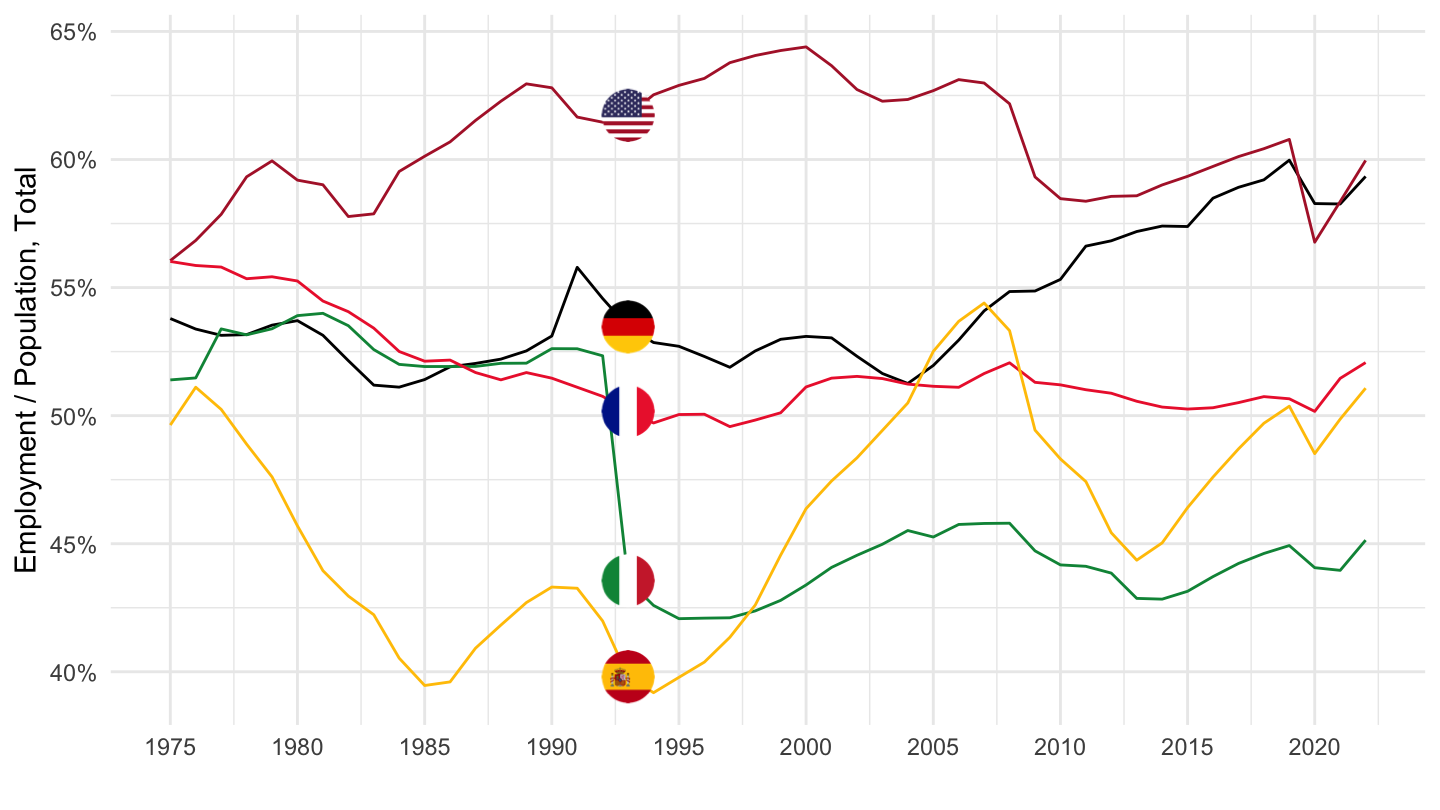
1995-
English
Code
LFS_SEXAGE_I_R %>%
  filter(SERIES == "EPR",
         AGE == "900000",
         SEX == "MW",
         COUNTRY %in% c("ITA", "DEU", "FRA", "ESP", "USA")) %>%
  year_to_date %>%
  filter(date >= as.Date("1995-01-01")) %>%
  left_join(LFS_SEXAGE_I_R_var$COUNTRY, by = "COUNTRY") %>%
  select(COUNTRY, Location = Country, date, obsValue) %>%
  left_join(colors, by = c("Location" = "country")) %>%
  mutate(color = ifelse(COUNTRY == "USA", color2, color)) %>%
  mutate(obsValue = obsValue/100) %>%
  ggplot(.) + geom_line(aes(x = date, y = obsValue, color = color)) +
  scale_color_identity() +
  theme_minimal() + xlab("") + ylab("Employment / Population, Total") +
  add_5flags +
  scale_x_date(breaks = seq(1960, 2100, 5) %>% paste0("-01-01") %>% as.Date,
               labels = date_format("%Y")) +
  theme(legend.position = "none") +
  scale_y_continuous(breaks = 0.01*seq(0, 200, 5),
                     labels = scales::percent_format(accuracy = 1))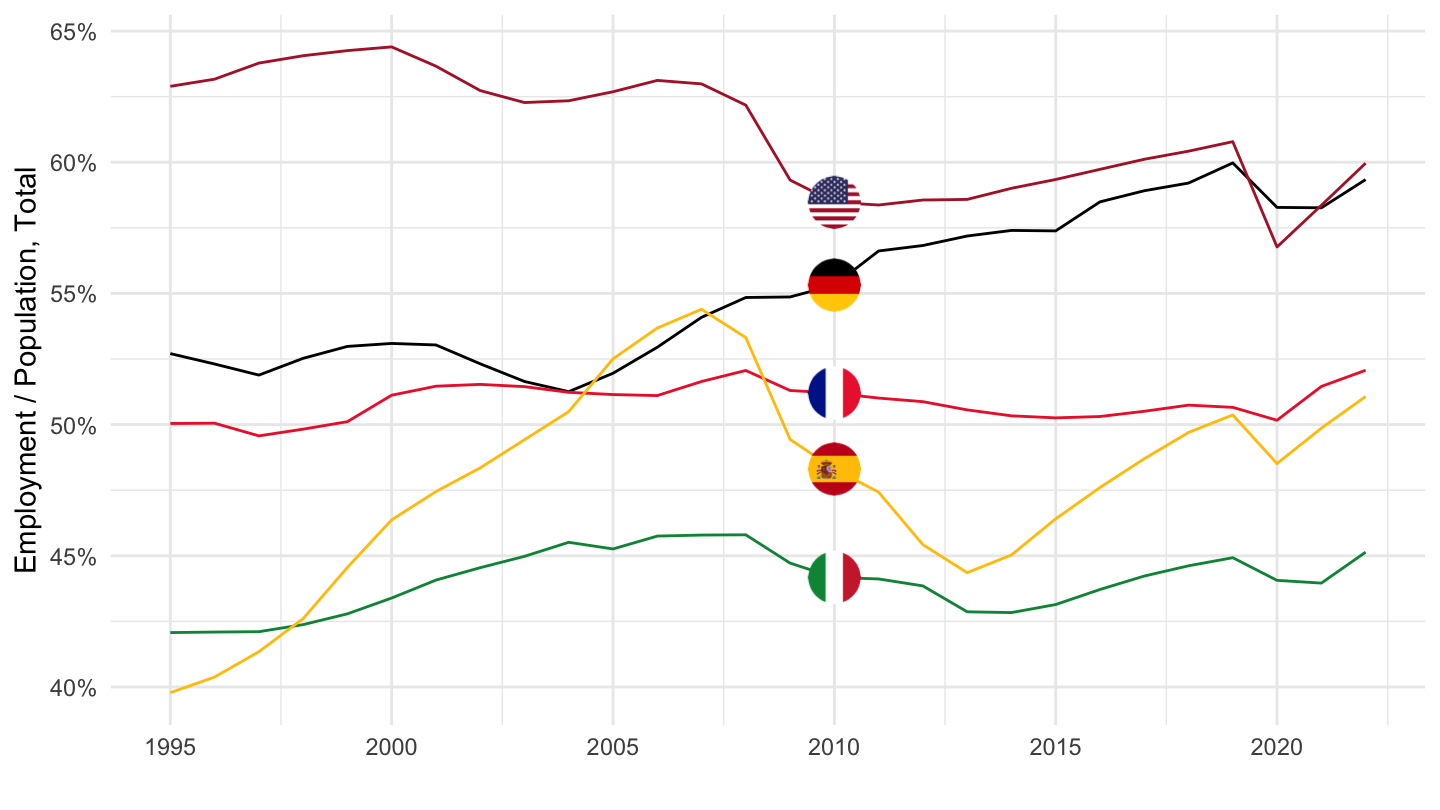
French
Code
LFS_SEXAGE_I_R %>%
  filter(SERIES == "EPR",
         AGE == "900000",
         SEX == "MW",
         COUNTRY %in% c("ITA", "DEU", "FRA", "ESP", "USA")) %>%
  year_to_date %>%
  filter(date >= as.Date("1995-01-01")) %>%
  left_join(LFS_SEXAGE_I_R_var$COUNTRY, by = "COUNTRY") %>%
  select(COUNTRY, Location = Country, date, obsValue) %>%
  left_join(colors, by = c("Location" = "country")) %>%
  mutate(color = ifelse(COUNTRY == "USA", color2, color)) %>%
  mutate(obsValue = obsValue/100) %>%
  ggplot(.) + geom_line(aes(x = date, y = obsValue, color = color)) +
  scale_color_identity() +
  theme_minimal() + xlab("") + ylab("Taux d'emploi") +
  add_5flags +
  scale_x_date(breaks = seq(1960, 2100, 5) %>% paste0("-01-01") %>% as.Date,
               labels = date_format("%Y")) +
  theme(legend.position = "none") +
  scale_y_continuous(breaks = 0.01*seq(0, 200, 5),
                     labels = scales::percent_format(accuracy = 1))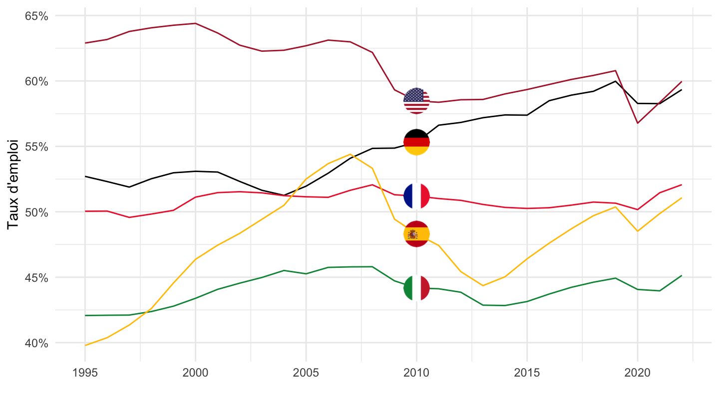
Germany, France, Italy, Greece, Spain
Total
Code
LFS_SEXAGE_I_R %>%
  filter(SERIES == "EPR",
         AGE == "900000",
         SEX == "MW",
         COUNTRY %in% c("ITA", "DEU", "FRA", "ESP", "GRC")) %>%
  year_to_date %>%
  left_join(LFS_SEXAGE_I_R_var$COUNTRY, by = "COUNTRY") %>%
  select(Location = Country, date, obsValue) %>%
  left_join(colors, by = c("Location" = "country")) %>%
  mutate(obsValue = obsValue/100) %>%
  ggplot(.) + geom_line(aes(x = date, y = obsValue, color = color)) +
  scale_color_identity() +
  theme_minimal() + xlab("") + ylab("Employment / Population, Total") +
  add_5flags +
  scale_x_date(breaks = seq(1960, 2100, 2) %>% paste0("-01-01") %>% as.Date,
               labels = date_format("%Y")) +
  theme(legend.position = "none") +
  scale_y_continuous(breaks = 0.01*seq(0, 200, 5),
                     labels = scales::percent_format(accuracy = 1))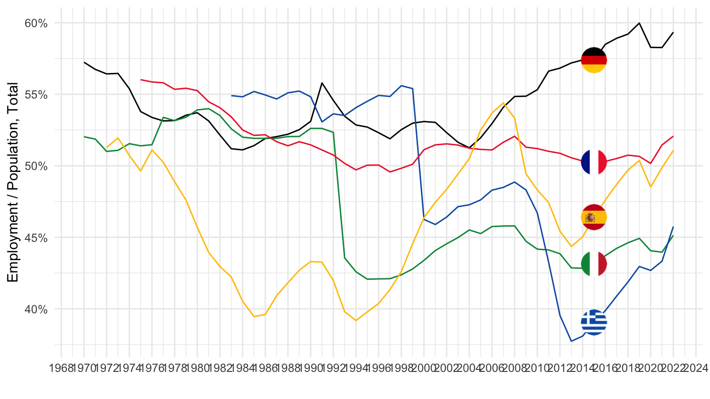
25-64
All
Code
LFS_SEXAGE_I_R %>%
  filter(SERIES == "EPR",
         AGE == "2564",
         SEX == "MW",
         COUNTRY %in% c("ITA", "DEU", "FRA", "ESP", "GRC")) %>%
  year_to_date %>%
  left_join(LFS_SEXAGE_I_R_var$COUNTRY, by = "COUNTRY") %>%
  select(Country, date, obsValue) %>%
  arrange(Country, date) %>%
  ggplot(.) + geom_line(aes(x = date, y = obsValue/100, color = Country)) +
  scale_color_manual(values = c("#ED2939", "#000000", "#0D5EAF", "#009246", "#FFC400")) +
  theme_minimal() + xlab("") + ylab("Employment / Population, 25-64") +
  geom_image(data = . %>%
               filter(date == as.Date("2012-01-01")) %>%
               mutate(date = as.Date("2012-01-01"),
                      image = paste0("../../icon/flag/round/", str_to_lower(Country), ".png")),
             aes(x = date, y = obsValue/100, image = image), asp = 1.5) +
  scale_x_date(breaks = seq(1960, 2100, 2) %>% paste0("-01-01") %>% as.Date,
               labels = date_format("%Y")) +
  theme(legend.position = "none") +
  scale_y_continuous(breaks = 0.01*seq(0, 200, 5),
                     labels = scales::percent_format(accuracy = 1))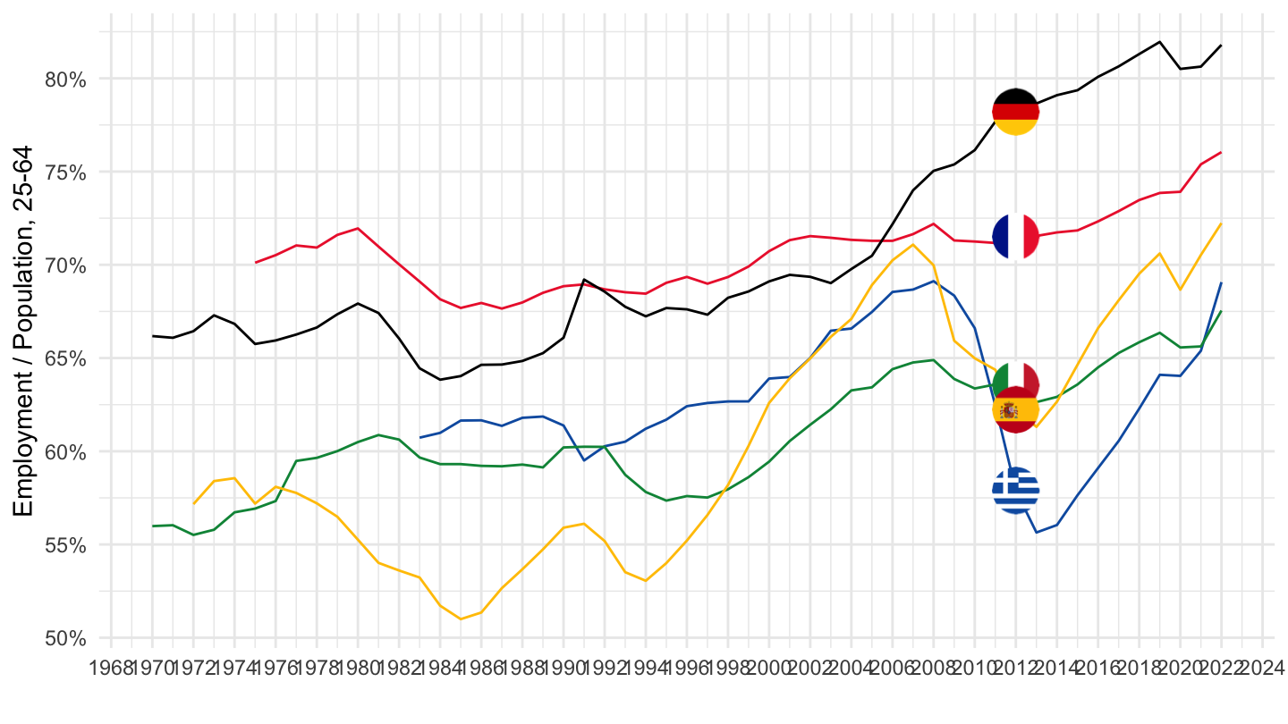
2000-
Code
LFS_SEXAGE_I_R %>%
  filter(SERIES == "EPR",
         AGE == "2564",
         SEX == "MW",
         COUNTRY %in% c("ITA", "DEU", "FRA", "ESP", "GRC")) %>%
  year_to_date %>%
  filter(date >= as.Date("2000-01-01")) %>%
  left_join(LFS_SEXAGE_I_R_var$COUNTRY, by = "COUNTRY") %>%
  select(Country, date, obsValue) %>%
  arrange(Country, date) %>%
  ggplot(.) + geom_line(aes(x = date, y = obsValue/100, color = Country)) +
  scale_color_manual(values = c("#ED2939", "#000000", "#0D5EAF", "#009246", "#FFC400")) +
  theme_minimal() + xlab("") + ylab("Employment / Population, 25-64") +
  geom_image(data = . %>%
               filter(date == as.Date("2012-01-01")) %>%
               mutate(date = as.Date("2012-01-01"),
                      image = paste0("../../icon/flag/round/", str_to_lower(Country), ".png")),
             aes(x = date, y = obsValue/100, image = image), asp = 1.5) +
  scale_x_date(breaks = seq(1960, 2100, 2) %>% paste0("-01-01") %>% as.Date,
               labels = date_format("%Y")) +
  theme(legend.position = "none") +
  scale_y_continuous(breaks = 0.01*seq(0, 200, 5),
                     labels = scales::percent_format(accuracy = 1))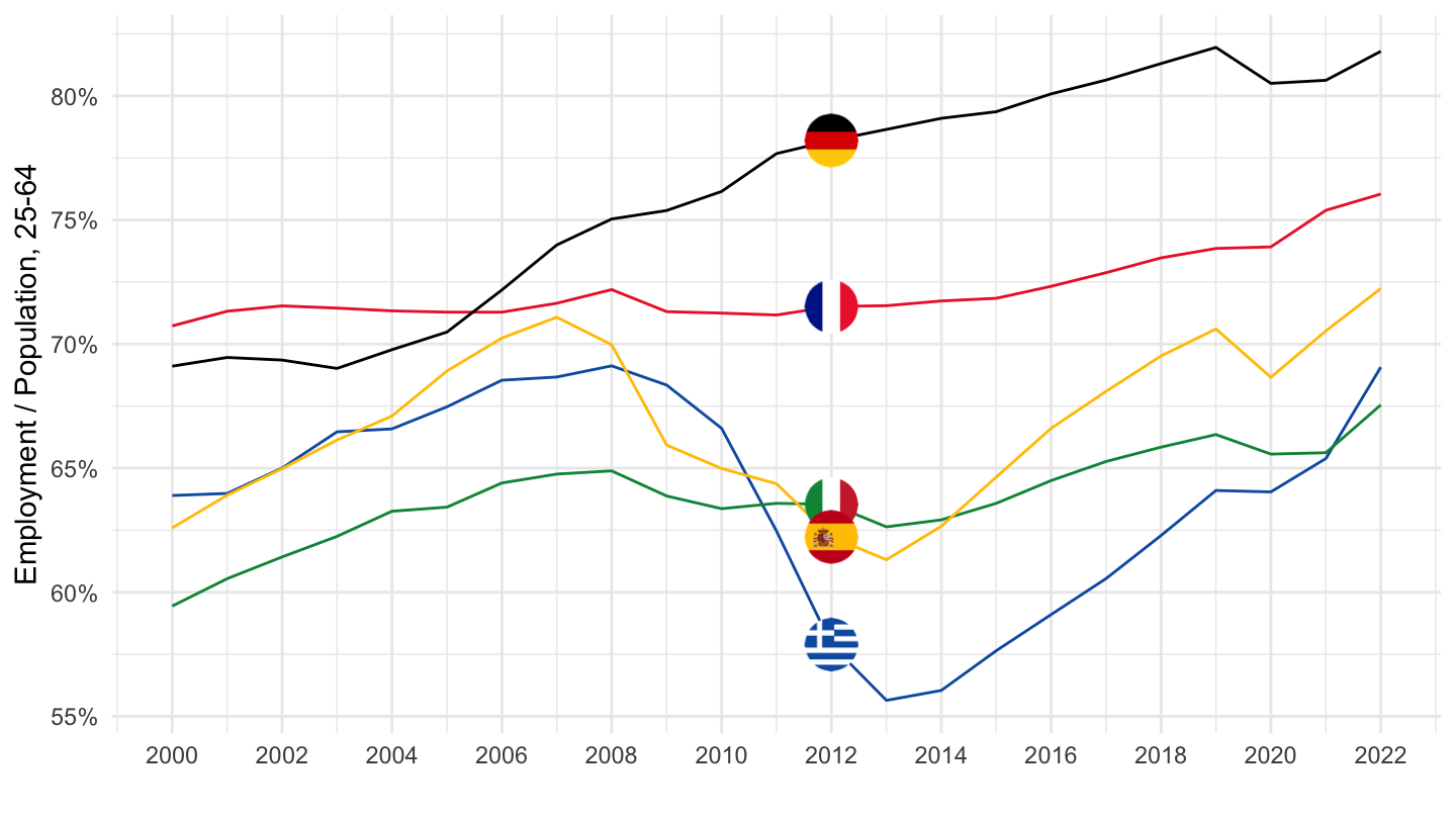
15-64
All
Code
LFS_SEXAGE_I_R %>%
  filter(SERIES == "EPR",
         AGE == "1564",
         SEX == "MW",
         COUNTRY %in% c("ITA", "DEU", "FRA", "ESP", "GRC")) %>%
  year_to_date %>%
  left_join(LFS_SEXAGE_I_R_var$COUNTRY, by = "COUNTRY") %>%
  select(Country, date, obsValue) %>%
  arrange(Country, date) %>%
  ggplot(.) + geom_line(aes(x = date, y = obsValue/100, color = Country)) +
  scale_color_manual(values = c("#ED2939", "#000000", "#0D5EAF", "#009246", "#FFC400")) +
  theme_minimal() + xlab("") + ylab("Employment / Population, 25-64") +
  geom_image(data = . %>%
               filter(date == as.Date("2012-01-01")) %>%
               mutate(date = as.Date("2012-01-01"),
                      image = paste0("../../icon/flag/round/", str_to_lower(Country), ".png")),
             aes(x = date, y = obsValue/100, image = image), asp = 1.5) +
  scale_x_date(breaks = seq(1960, 2100, 2) %>% paste0("-01-01") %>% as.Date,
               labels = date_format("%Y")) +
  theme(legend.position = "none") +
  scale_y_continuous(breaks = 0.01*seq(0, 200, 5),
                     labels = scales::percent_format(accuracy = 1))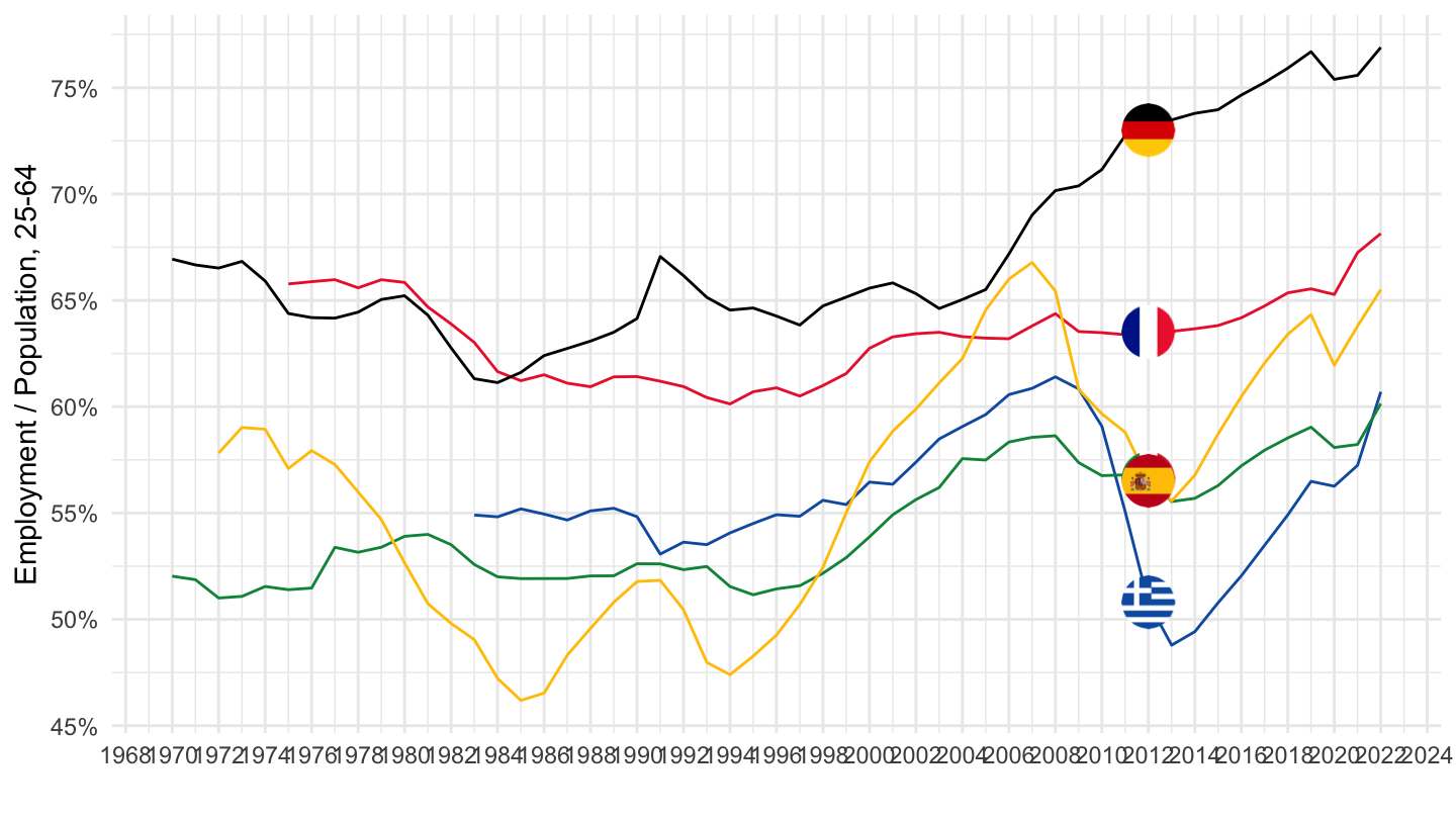
2002-
Code
LFS_SEXAGE_I_R %>%
  filter(SERIES == "EPR",
         AGE == "1564",
         SEX == "MW",
         COUNTRY %in% c("ITA", "DEU", "FRA", "ESP", "USA")) %>%
  year_to_date %>%
  filter(date >= as.Date("2000-01-01")) %>%
  left_join(LFS_SEXAGE_I_R_var$COUNTRY, by = "COUNTRY") %>%
  select(Country, date, obsValue) %>%
  arrange(Country, date) %>%
  mutate(obsValue = obsValue/100) %>%
  rename(Location = Country) %>%
  left_join(colors, by = c("Location" = "country")) %>%
  mutate(color = ifelse(Location ==  "United States", color2, color)) %>%
  ggplot(.) + geom_line(aes(x = date, y = obsValue, color = color)) +
  scale_color_identity() +
  theme_minimal() + xlab("") + ylab("Employment / Population, 15-64") +
  add_5flags +
  scale_x_date(breaks = seq(1960, 2022, 2) %>% paste0("-01-01") %>% as.Date,
               labels = date_format("%Y")) +
  theme(legend.position = "none") +
  scale_y_continuous(breaks = 0.01*seq(0, 200, 5),
                     labels = scales::percent_format(accuracy = 1))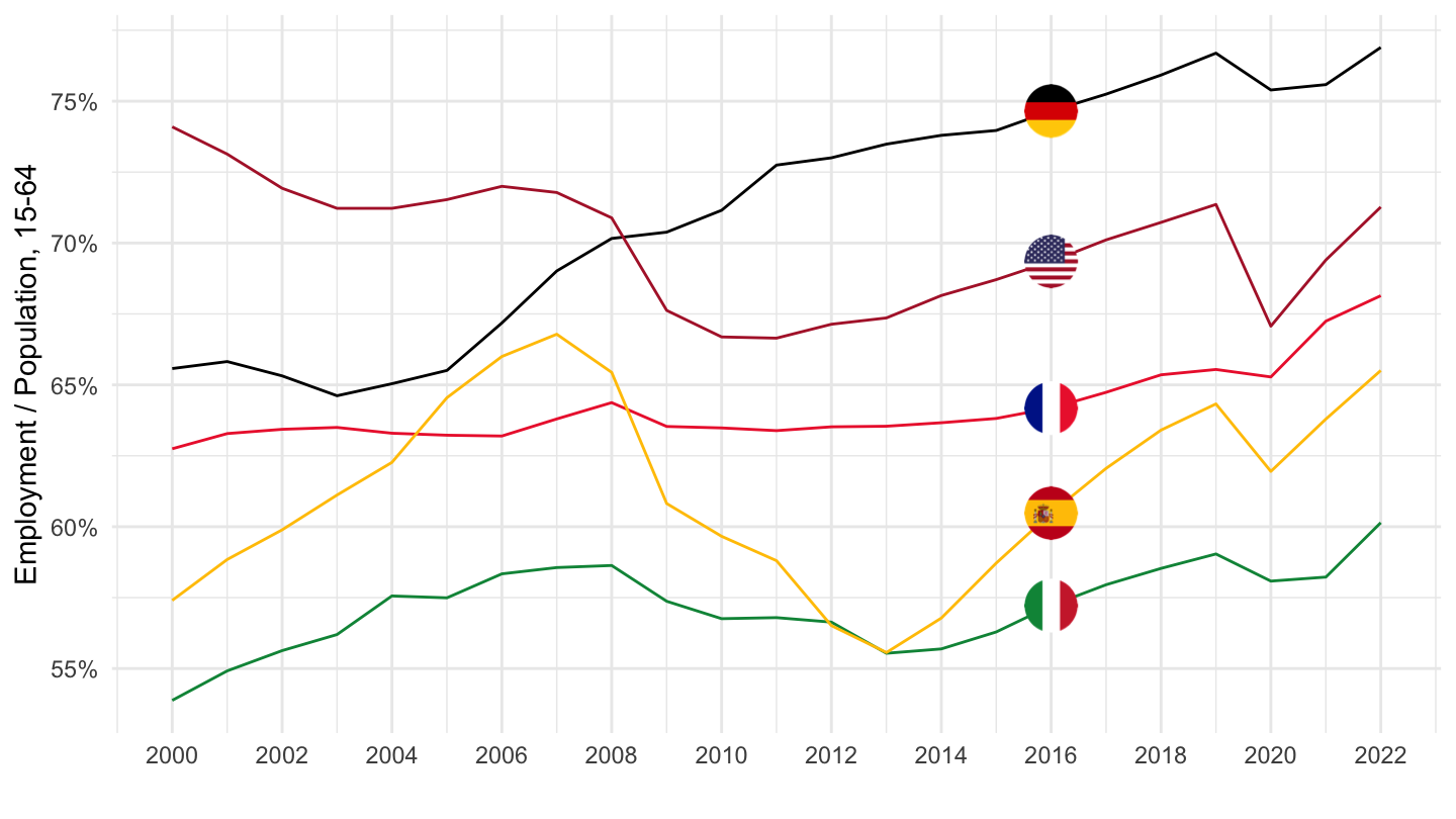
Unemployment rate, 25-64
Code
LFS_SEXAGE_I_R %>%
  filter(SERIES == "UR",
         AGE == "2564",
         SEX == "MW",
         COUNTRY %in% c("ITA", "DEU", "FRA", "ESP", "GRC")) %>%
  year_to_date %>%
  filter(date >= as.Date("2000-01-01")) %>%
  left_join(LFS_SEXAGE_I_R_var$COUNTRY, by = "COUNTRY") %>%
  select(Country, date, obsValue) %>%
  arrange(Country, date) %>%
  ggplot(.) + geom_line(aes(x = date, y = obsValue/100, color = Country)) +
  scale_color_manual(values = c("#ED2939", "#000000", "#0D5EAF", "#009246", "#FFC400")) +
  theme_minimal() + xlab("") + ylab("Unemployment Rate, 25-64") +
  geom_image(data = . %>%
               filter(date == as.Date("2014-01-01")) %>%
               mutate(date = as.Date("2014-01-01"),
                      image = paste0("../../icon/flag/round/", str_to_lower(Country), ".png")),
             aes(x = date, y = obsValue/100, image = image), asp = 1.5) +
  scale_x_date(breaks = seq(1960, 2100, 2) %>% paste0("-01-01") %>% as.Date,
               labels = date_format("%Y")) +
  theme(legend.position = "none") +
  scale_y_continuous(breaks = 0.01*seq(0, 200, 2),
                     labels = scales::percent_format(accuracy = 1))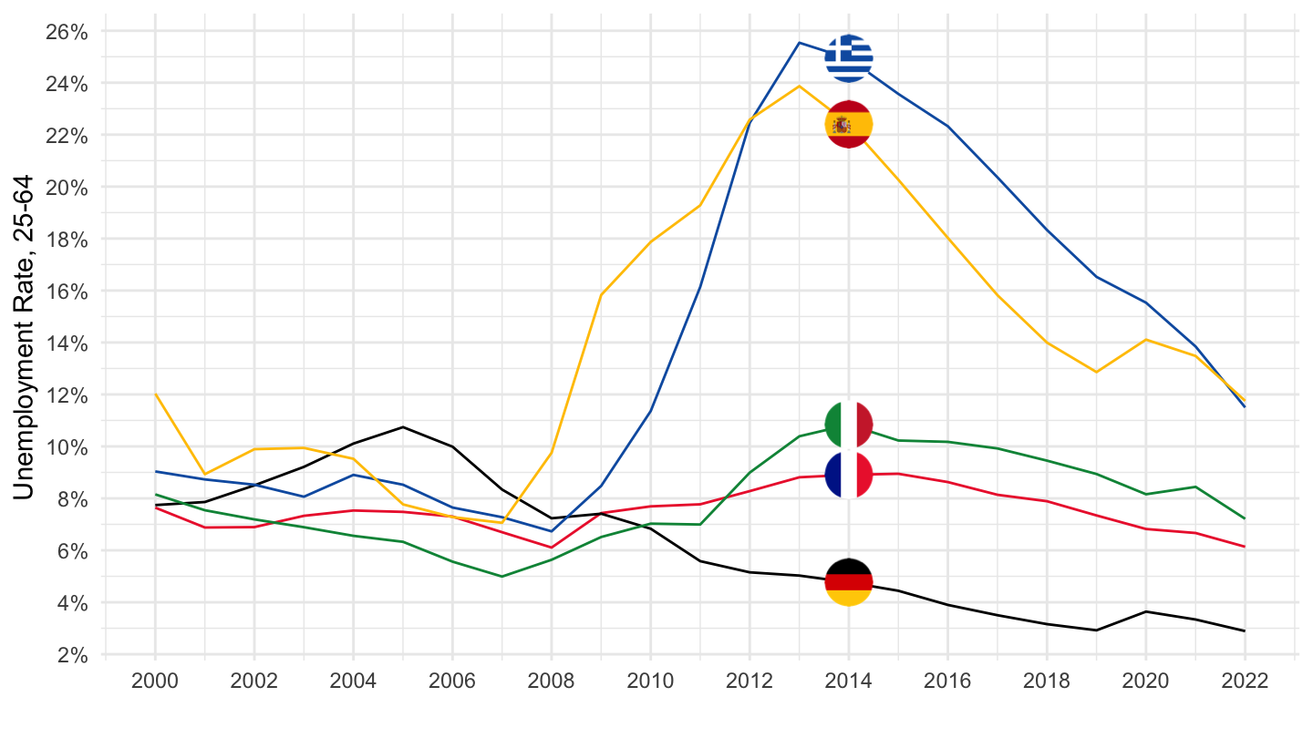
Unemployment rate, 15-24
Code
LFS_SEXAGE_I_R %>%
  filter(SERIES == "UR",
         AGE == "1524",
         SEX == "MW",
         COUNTRY %in% c("ITA", "DEU", "FRA", "ESP", "GRC")) %>%
  year_to_date %>%
  filter(date >= as.Date("2000-01-01")) %>%
  left_join(LFS_SEXAGE_I_R_var$COUNTRY, by = "COUNTRY") %>%
  select(Country, date, obsValue) %>%
  arrange(Country, date) %>%
  ggplot(.) + geom_line(aes(x = date, y = obsValue/100, color = Country)) +
  scale_color_manual(values = c("#ED2939", "#000000", "#0D5EAF", "#009246", "#FFC400")) +
  theme_minimal() + xlab("") + ylab("Unemployment Rate, 15-24") +
  geom_image(data = . %>%
               filter(date == as.Date("2013-01-01")) %>%
               mutate(date = as.Date("2013-01-01"),
                      image = paste0("../../icon/flag/round/", str_to_lower(Country), ".png")),
             aes(x = date, y = obsValue/100, image = image), asp = 1.5) +
  scale_x_date(breaks = seq(1960, 2100, 2) %>% paste0("-01-01") %>% as.Date,
               labels = date_format("%Y")) +
  theme(legend.position = "none") +
  scale_y_continuous(breaks = 0.01*seq(0, 200, 5),
                     labels = scales::percent_format(accuracy = 1))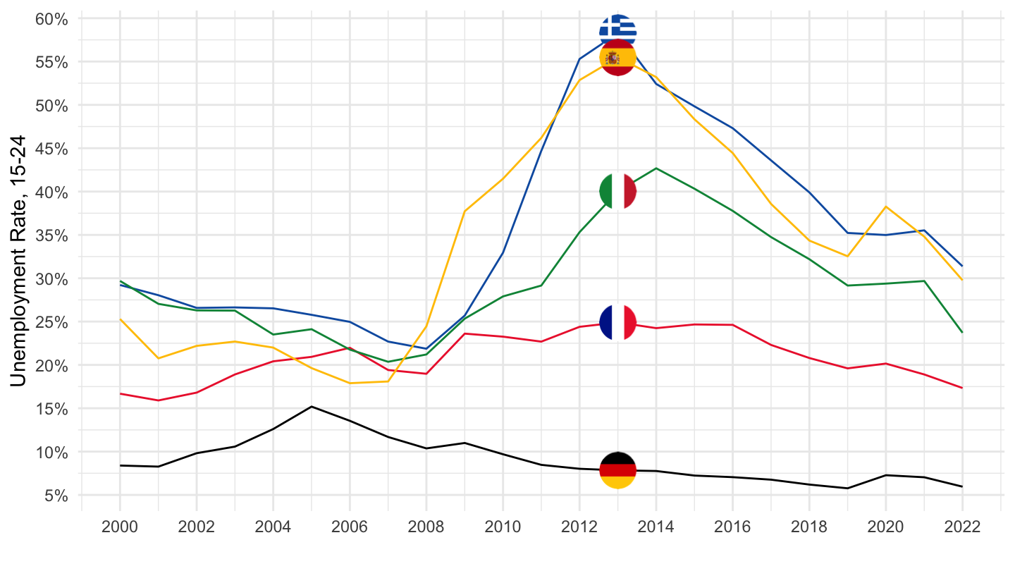
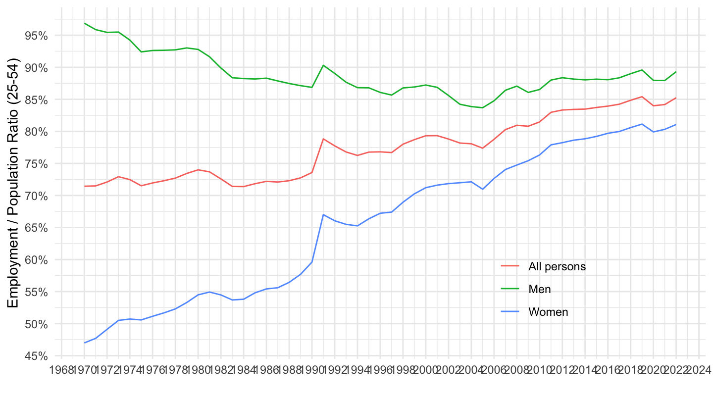
Employment / Population, Men, 25-54
Number of observations
Code
LFS_SEXAGE_I_R %>%
  filter(SERIES == "EPR",
         AGE == "2554",
         SEX == "MEN") %>%
  left_join(LFS_SEXAGE_I_R_var$COUNTRY, by = "COUNTRY") %>%
  group_by(COUNTRY, Country) %>%
  summarise(Nobs = n()) %>%
  arrange(-Nobs) %>%
  mutate(Flag = gsub(" ", "-", str_to_lower(gsub(" ", "-", Country))),
         Flag = paste0('<img src="../../icon/flag/round/vsmall/', Flag, '.png" alt="Flag">')) %>%
  select(Flag, everything()) %>%
  {if (is_html_output()) datatable(., filter = 'top', rownames = F, escape = F) else .}
Table: 1970, 1980, 1990, 2000, 2010
Code
LFS_SEXAGE_I_R %>%
  filter(SERIES == "EPR",
         AGE == "2554",
         SEX == "MEN",
         obsTime %in% c("1970", "1980", "1990", "2000", "2010")) %>%
  left_join(LFS_SEXAGE_I_R_var$COUNTRY, by = "COUNTRY") %>%
  select(COUNTRY, Country, obsTime, obsValue) %>%
  mutate(obsValue = round(obsValue, 1)) %>%
  spread(obsTime, obsValue) %>%
  mutate(Flag = gsub(" ", "-", str_to_lower(gsub(" ", "-", Country))),
         Flag = paste0('<img src="../../icon/flag/round/vsmall/', Flag, '.png" alt="Flag">')) %>%
  select(Flag, everything()) %>%
  {if (is_html_output()) datatable(., filter = 'top', rownames = F, escape = F) else .}
Table: 2003, 2007, 2011, 2015, 2019
Code
LFS_SEXAGE_I_R %>%
  filter(SERIES == "EPR",
         AGE == "2554",
         SEX == "MEN",
         obsTime %in% c("2003", "2007", "2011", "2015", "2019")) %>%
  left_join(LFS_SEXAGE_I_R_var$COUNTRY, by = "COUNTRY") %>%
  select(COUNTRY, Country, obsTime, obsValue) %>%
  mutate(obsValue = round(obsValue, 1)) %>%
  spread(obsTime, obsValue) %>%
  arrange(-`2019`) %>%
  mutate(Flag = gsub(" ", "-", str_to_lower(gsub(" ", "-", Country))),
         Flag = paste0('<img src="../../icon/flag/round/vsmall/', Flag, '.png" alt="Flag">')) %>%
  select(Flag, everything()) %>%
  {if (is_html_output()) datatable(., filter = 'top', rownames = F, escape = F) else .}
Germany, France, Italy, Greece, United States
1960-
Code
LFS_SEXAGE_I_R %>%
  filter(SERIES == "EPR",
         AGE == "2554",
         SEX == "MEN",
         COUNTRY %in% c("ITA", "DEU", "FRA", "GRC", "USA")) %>%
  year_to_date %>%
  filter(date >= as.Date("1960-01-01")) %>%
  left_join(LFS_SEXAGE_I_R_var$COUNTRY, by = "COUNTRY") %>%
  select(Country, date, obsValue) %>%
  arrange(Country, date) %>%
  ggplot(.) + geom_line(aes(x = date, y = obsValue/100, color = Country)) +
  scale_color_manual(values = c("#002395", "#000000", "#0D5EAF", "#009246", "#B22234")) +
  theme_minimal() + xlab("") + ylab("Employment / Population, Men, 25-54") +
  geom_image(data = . %>%
               filter(date == as.Date("2013-01-01")) %>%
               mutate(image = paste0("../../icon/flag/round/", str_to_lower(gsub(" ", "-", Country)), ".png")),
             aes(x = date, y = obsValue/100, image = image), asp = 1.5) +
  scale_x_date(breaks = seq(1960, 2100, 5) %>% paste0("-01-01") %>% as.Date,
               labels = date_format("%Y")) +
  theme(legend.position = "none") +
  scale_y_continuous(breaks = 0.01*seq(0, 200, 5),
                     labels = scales::percent_format(accuracy = 1))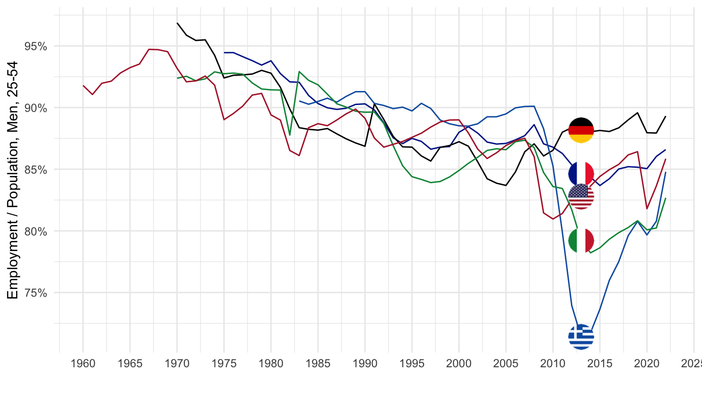
2000-
Code
LFS_SEXAGE_I_R %>%
  filter(SERIES == "EPR",
         AGE == "2554",
         SEX == "MEN",
         COUNTRY %in% c("ITA", "ESP", "FRA", "GRC", "USA")) %>%
  year_to_date %>%
  filter(date >= as.Date("2000-01-01")) %>%
  left_join(LFS_SEXAGE_I_R_var$COUNTRY, by = "COUNTRY") %>%
  select(Country, date, obsValue) %>%
  arrange(Country, date) %>%
  ggplot(.) + geom_line(aes(x = date, y = obsValue/100, color = Country)) +
  scale_color_manual(values = c("#002395", "#0D5EAF", "#009246", "#FFC400", "#B22234")) +
  theme_minimal() + xlab("") + ylab("Employment / Population, Men, 25-54") +
  geom_image(data = . %>%
               filter(date == as.Date("2011-01-01")) %>%
               mutate(image = paste0("../../icon/flag/round/", str_to_lower(gsub(" ", "-", Country)), ".png")),
             aes(x = date, y = obsValue/100, image = image), asp = 1.5) +
  scale_x_date(breaks = seq(1960, 2100, 2) %>% paste0("-01-01") %>% as.Date,
               labels = date_format("%Y")) +
  theme(legend.position = "none") +
  scale_y_continuous(breaks = 0.01*seq(0, 200, 2),
                     labels = scales::percent_format(accuracy = 1))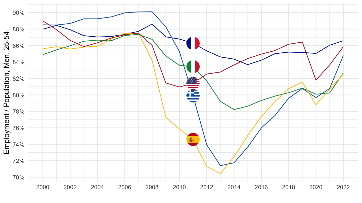
Germany, France, Italy, Greece, Spain
1960-
Code
LFS_SEXAGE_I_R %>%
  filter(SERIES == "EPR",
         AGE == "2554",
         SEX == "MEN",
         COUNTRY %in% c("ITA", "DEU", "FRA", "ESP", "USA")) %>%
  year_to_date %>%
  filter(date >= as.Date("1960-01-01")) %>%
  left_join(LFS_SEXAGE_I_R_var$COUNTRY, by = "COUNTRY") %>%
  select(Country, date, obsValue) %>%
  arrange(Country, date) %>%
  ggplot(.) + geom_line(aes(x = date, y = obsValue/100, color = Country)) +
  scale_color_manual(values = c("#ED2939", "#000000", "#0D5EAF", "#009246", "#FFC400")) +
  theme_minimal() + xlab("") + ylab("Employment / Population, Men, 25-54") +
  geom_image(data = . %>%
               filter(date == as.Date("2012-01-01")) %>%
               mutate(date = as.Date("2012-01-01"),
                      image = paste0("../../icon/flag/round/", str_to_lower(gsub(" ", "-", Country)), ".png")),
             aes(x = date, y = obsValue/100, image = image), asp = 1.5) +
  scale_x_date(breaks = seq(1960, 2100, 5) %>% paste0("-01-01") %>% as.Date,
               labels = date_format("%Y")) +
  theme(legend.position = "none") +
  scale_y_continuous(breaks = 0.01*seq(0, 200, 5),
                     labels = scales::percent_format(accuracy = 1))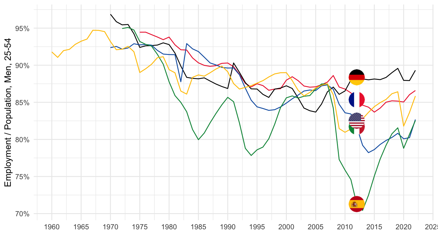
2000-
Code
LFS_SEXAGE_I_R %>%
  filter(SERIES == "EPR",
         AGE == "2554",
         SEX == "MEN",
         COUNTRY %in% c("ITA", "DEU", "FRA", "ESP", "GRC")) %>%
  year_to_date %>%
  filter(date >= as.Date("2000-01-01")) %>%
  left_join(LFS_SEXAGE_I_R_var$COUNTRY, by = "COUNTRY") %>%
  select(Country, date, obsValue) %>%
  arrange(Country, date) %>%
  ggplot(.) + geom_line(aes(x = date, y = obsValue/100, color = Country)) +
  scale_color_manual(values = c("#ED2939", "#000000", "#0D5EAF", "#009246", "#FFC400")) +
  theme_minimal() + xlab("") + ylab("Employment / Population, Men, 25-54") +
  geom_image(data = . %>%
               filter(date == as.Date("2012-01-01")) %>%
               mutate(date = as.Date("2012-01-01"),
                      image = paste0("../../icon/flag/round/", str_to_lower(gsub(" ", "-", Country)), ".png")),
             aes(x = date, y = obsValue/100, image = image), asp = 1.5) +
  scale_x_date(breaks = seq(1960, 2100, 2) %>% paste0("-01-01") %>% as.Date,
               labels = date_format("%Y")) +
  theme(legend.position = "none") +
  scale_y_continuous(breaks = 0.01*seq(0, 200, 5),
                     labels = scales::percent_format(accuracy = 1))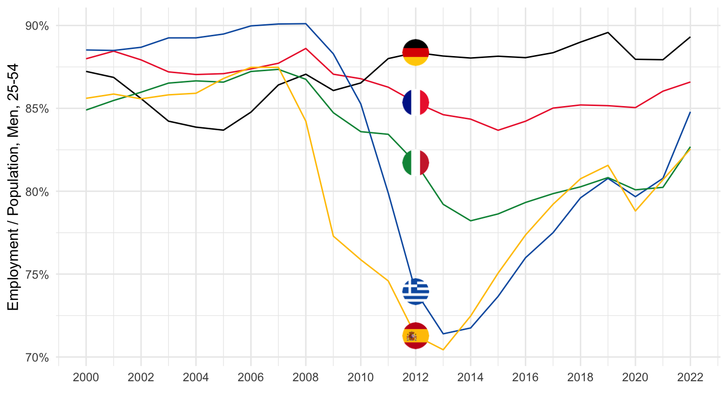
G7, North America, OECD, Oceania
Code
LFS_SEXAGE_I_R %>%
  filter(SERIES == "EPR",
         AGE == "2554",
         SEX == "MEN",
         COUNTRY %in% c("G7", "NAM", "OECD", "OCE")) %>%
  year_to_date %>%
  filter(date >= as.Date("1960-01-01")) %>%
  left_join(LFS_SEXAGE_I_R_var$COUNTRY, by = "COUNTRY") %>%
  select(Country, date, obsValue) %>%
  arrange(Country, date) %>%
  ggplot(.) + geom_line(aes(x = date, y = obsValue/100, color = Country)) +
  scale_color_manual(values = c("#002395", "#C60B1E", "#000000", "#009246")) +
  theme_minimal() + xlab("") + ylab("Employment / Population, Men, 25-54") +
  scale_x_date(breaks = seq(1960, 2100, 5) %>% paste0("-01-01") %>% as.Date,
               labels = date_format("%Y")) +
  theme(legend.position = c(0.2, 0.2)) +
  scale_y_continuous(breaks = 0.01*seq(0, 200, 2),
                     labels = scales::percent_format(accuracy = 1))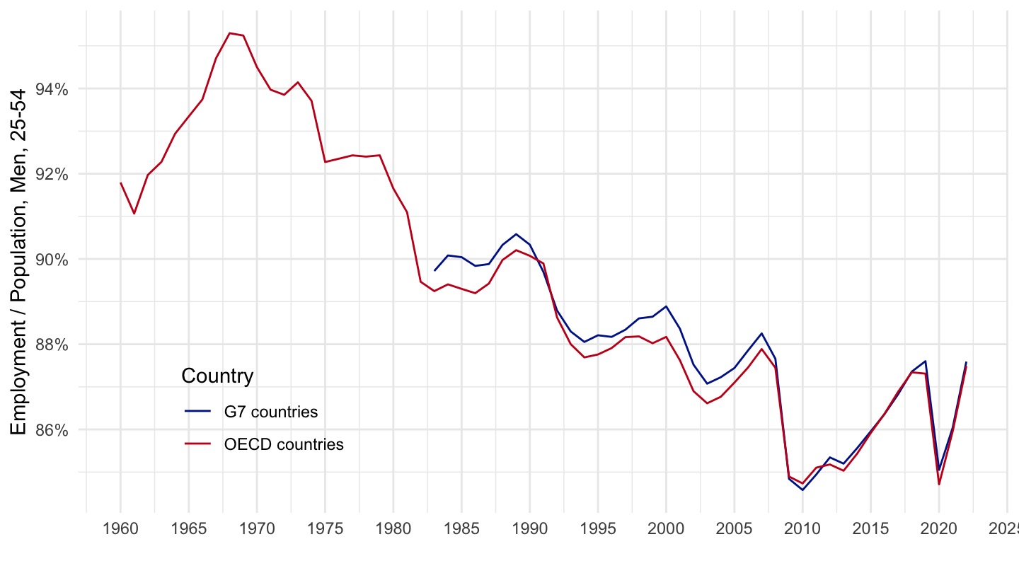
Germany, France, Italy
Code
LFS_SEXAGE_I_R %>%
  filter(SERIES == "EPR",
         AGE == "2554",
         SEX == "MEN",
         COUNTRY %in% c("ITA", "DEU", "FRA")) %>%
  year_to_date %>%
  filter(date >= as.Date("1960-01-01")) %>%
  left_join(LFS_SEXAGE_I_R_var$COUNTRY, by = "COUNTRY") %>%
  select(Country, date, obsValue) %>%
  arrange(Country, date) %>%
  ggplot(.) + geom_line(aes(x = date, y = obsValue/100, color = Country)) +
  scale_color_manual(values = c("#002395", "#000000", "#009246")) +
  theme_minimal() + xlab("") + ylab("Employment / Population, Men, 25-54") +
  geom_image(data = . %>%
               filter(date == as.Date("2019-01-01")) %>%
               mutate(date = as.Date("2021-01-01"),
                      image = paste0("../../icon/flag/round/", str_to_lower(Country), ".png")),
             aes(x = date, y = obsValue/100, image = image), asp = 1.5) +
  scale_x_date(breaks = seq(1960, 2100, 5) %>% paste0("-01-01") %>% as.Date,
               labels = date_format("%Y")) +
  theme(legend.position = "none") +
  scale_y_continuous(breaks = 0.01*seq(0, 200, 5),
                     labels = scales::percent_format(accuracy = 1))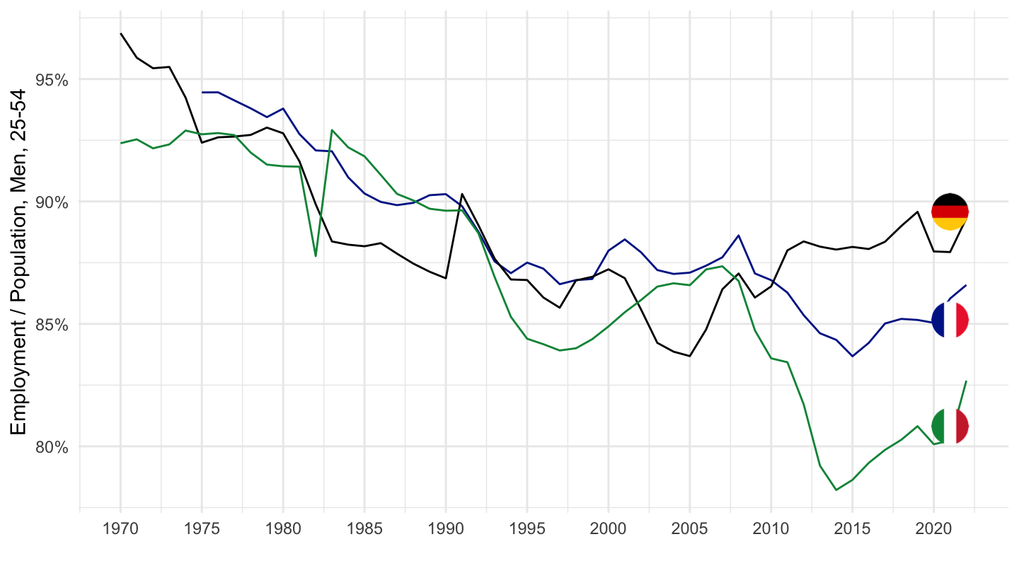
Europe, United States, United Kingdom
Code
LFS_SEXAGE_I_R %>%
  filter(SERIES == "EPR",
         AGE == "2554",
         SEX == "MEN",
         COUNTRY %in% c("EUR", "GBR", "USA")) %>%
  year_to_date %>%
  filter(date >= as.Date("1980-01-01")) %>%
  left_join(LFS_SEXAGE_I_R_var$COUNTRY, by = "COUNTRY") %>%
  select(Country, date, obsValue) %>%
  arrange(Country, date) %>%
  ggplot(.) + geom_line(aes(x = date, y = obsValue/100, color = Country)) +
  scale_color_manual(values = c("#FFCC00", "#CF142B", "#3C3B6E")) +
  theme_minimal() + xlab("") + ylab("Employment / Population, Men, 25-54") +
  geom_image(data = . %>%
               filter(date == as.Date("2019-01-01")) %>%
               mutate(date = as.Date("2021-01-01"),
                      image = paste0("../../icon/flag/round/", str_to_lower(gsub(" ", "-", Country)), ".png")),
             aes(x = date, y = obsValue/100, image = image), asp = 1.5) +
  scale_x_date(breaks = seq(1960, 2100, 5) %>% paste0("-01-01") %>% as.Date,
               labels = date_format("%Y")) +
  theme(legend.position = "none") +
  scale_y_continuous(breaks = 0.01*seq(0, 200, 1),
                     labels = scales::percent_format(accuracy = 1))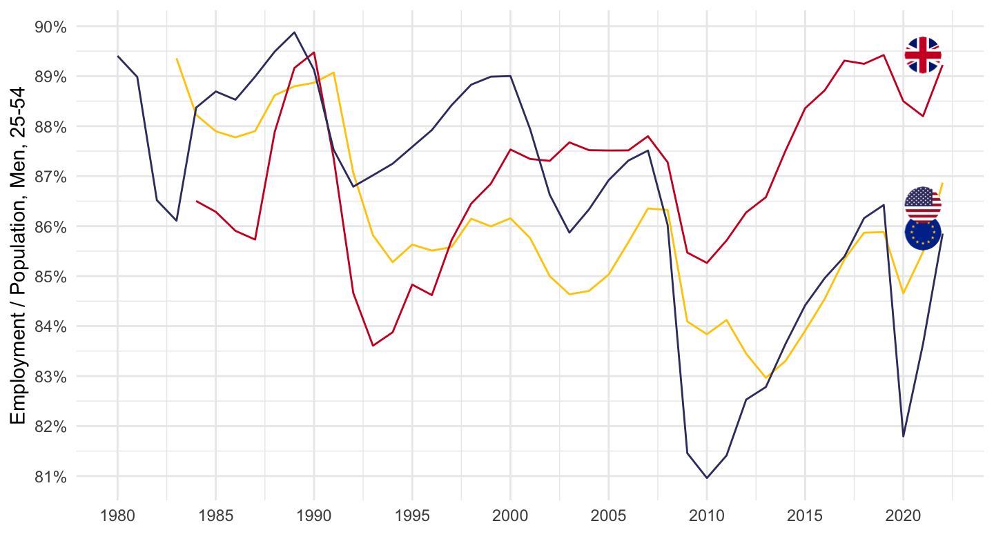
Europe, United States
Code
LFS_SEXAGE_I_R %>%
  filter(SERIES == "EPR",
         AGE == "2554",
         SEX == "MEN",
         COUNTRY %in% c("EUR", "EU16", "USA")) %>%
  year_to_date %>%
  filter(date >= as.Date("1960-01-01")) %>%
  left_join(LFS_SEXAGE_I_R_var$COUNTRY, by = "COUNTRY") %>%
  select(Country, date, obsValue) %>%
  arrange(Country, date) %>%
  ggplot(.) + geom_line(aes(x = date, y = obsValue/100, color = Country)) +
  scale_color_manual(values = c("#002395", "#000000", "#009246", "#B22234")) +
  theme_minimal() + xlab("") + ylab("Employment / Population, Men, 25-54") +
  scale_x_date(breaks = seq(1960, 2100, 5) %>% paste0("-01-01") %>% as.Date,
               labels = date_format("%Y")) +
  theme(legend.position = c(0.8, 0.8)) +
  scale_y_continuous(breaks = 0.01*seq(0, 200, 1),
                     labels = scales::percent_format(accuracy = 1))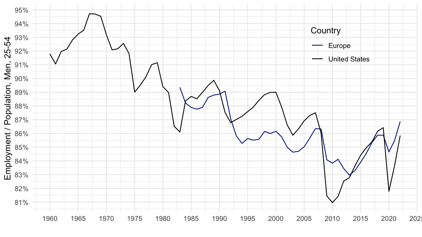
Germany, France, Italy, United States
Code
LFS_SEXAGE_I_R %>%
  filter(SERIES == "EPR",
         AGE == "2554",
         SEX == "MEN",
         COUNTRY %in% c("ITA", "DEU", "FRA", "USA")) %>%
  year_to_date %>%
  filter(date >= as.Date("1960-01-01")) %>%
  left_join(LFS_SEXAGE_I_R_var$COUNTRY, by = "COUNTRY") %>%
  select(Country, date, obsValue) %>%
  arrange(Country, date) %>%
  ggplot(.) + geom_line(aes(x = date, y = obsValue/100, color = Country)) +
  scale_color_manual(values = c("#002395", "#000000", "#009246", "#B22234")) +
  theme_minimal() + xlab("") + ylab("Employment / Population, Men, 25-54") +
  geom_image(data = . %>%
               filter(date == as.Date("2019-01-01")) %>%
               mutate(date = as.Date("2021-01-01"),
                      image = paste0("../../icon/flag/round/", str_to_lower(gsub(" ", "-", Country)), ".png")),
             aes(x = date, y = obsValue/100, image = image), asp = 1.5) +
  scale_x_date(breaks = seq(1960, 2100, 5) %>% paste0("-01-01") %>% as.Date,
               labels = date_format("%Y")) +
  theme(legend.position = "none") +
  scale_y_continuous(breaks = 0.01*seq(0, 200, 5),
                     labels = scales::percent_format(accuracy = 1))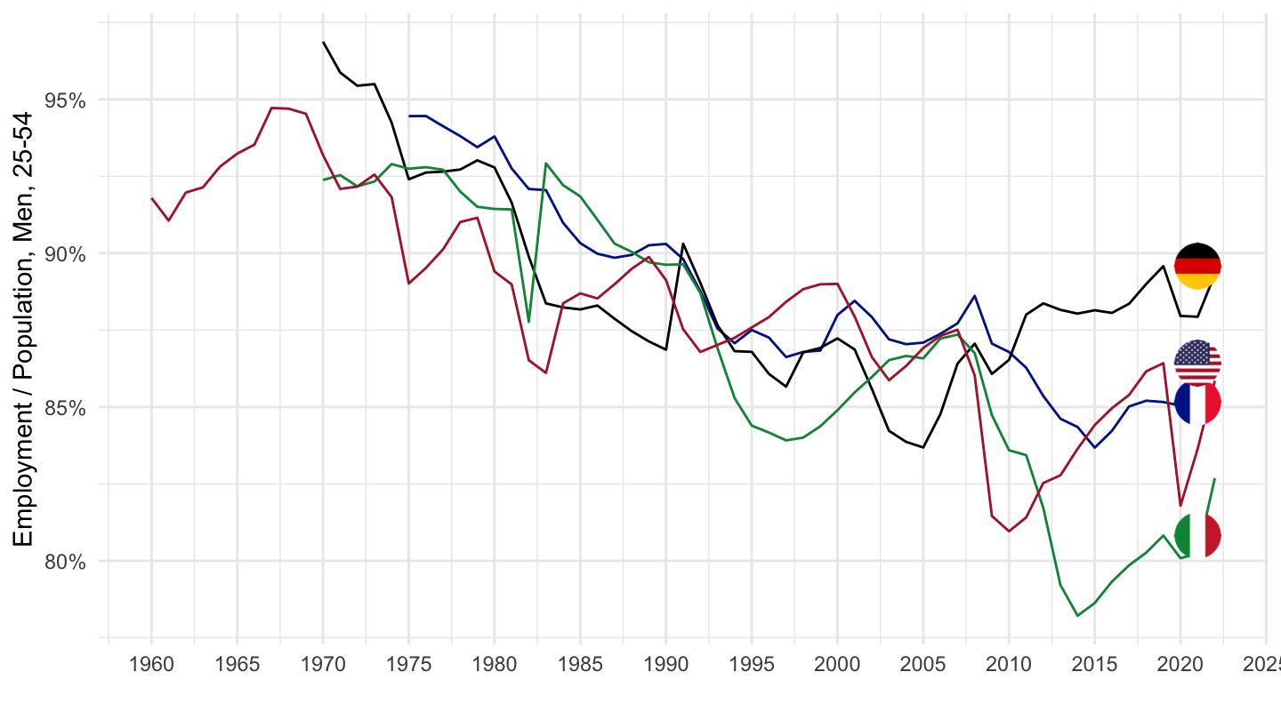
Finland, Sweden, United States
Code
LFS_SEXAGE_I_R %>%
  filter(SERIES == "EPR",
         AGE == "2554",
         SEX == "MEN",
         COUNTRY %in% c("USA", "FIN", "SWE")) %>%
  year_to_date %>%
  filter(date >= as.Date("1960-01-01")) %>%
  left_join(LFS_SEXAGE_I_R_var$COUNTRY, by = "COUNTRY") %>%
  select(Country, date, obsValue) %>%
  arrange(Country, date) %>%
  ggplot(.) + geom_line(aes(x = date, y = obsValue/100, color = Country)) +
  scale_color_manual(values = c("#003580", "#FECC00", "#B22234")) +
  theme_minimal() + xlab("") + ylab("Employment / Population, Men, 25-54") +
  geom_image(data = . %>%
               filter(date == as.Date("2019-01-01")) %>%
               mutate(date = as.Date("2021-01-01"),
                      image = paste0("../../icon/flag/round/", str_to_lower(gsub(" ", "-", Country)), ".png")),
             aes(x = date, y = obsValue/100, image = image), asp = 1.5) +
  scale_x_date(breaks = seq(1960, 2100, 5) %>% paste0("-01-01") %>% as.Date,
               labels = date_format("%Y")) +
  theme(legend.position = "none") +
  scale_y_continuous(breaks = 0.01*seq(0, 200, 2),
                     labels = scales::percent_format(accuracy = 1))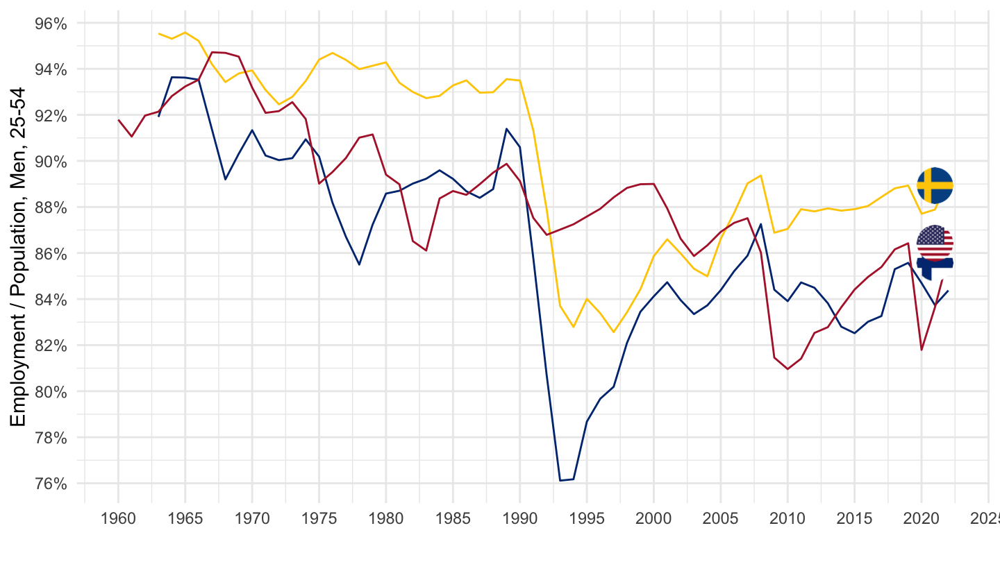
Australia, Germany, Japan
Code
LFS_SEXAGE_I_R %>%
  filter(SERIES == "EPR",
         AGE == "2554",
         SEX == "MEN",
         COUNTRY %in% c("AUS", "JPN", "DEU")) %>%
  year_to_date %>%
  filter(date >= as.Date("1960-01-01")) %>%
  left_join(LFS_SEXAGE_I_R_var$COUNTRY, by = "COUNTRY") %>%
  select(Country, date, obsValue) %>%
  arrange(Country, date) %>%
  ggplot(.) + geom_line(aes(x = date, y = obsValue/100, color = Country)) +
  scale_color_manual(values = c("#00008B", "#000000", "#BC002D")) +
  theme_minimal() + xlab("") + ylab("Employment / Population, Men, 25-54") +
  geom_image(data = . %>%
               filter(date == as.Date("2019-01-01")) %>%
               mutate(date = as.Date("2021-01-01"),
                      image = paste0("../../icon/flag/round/", str_to_lower(gsub(" ", "-", Country)), ".png")),
             aes(x = date, y = obsValue/100, image = image), asp = 1.5) +
  scale_x_date(breaks = seq(1960, 2100, 5) %>% paste0("-01-01") %>% as.Date,
               labels = date_format("%Y")) +
  theme(legend.position = "none") +
  scale_y_continuous(breaks = 0.01*seq(0, 200, 2),
                     labels = scales::percent_format(accuracy = 1))
Italy, Netherlands, Spain
Code
LFS_SEXAGE_I_R %>%
  filter(SERIES == "EPR",
         AGE == "2554",
         SEX == "MEN",
         COUNTRY %in% c("ITA", "NLD", "ESP")) %>%
  year_to_date %>%
  filter(date >= as.Date("1960-01-01")) %>%
  left_join(LFS_SEXAGE_I_R_var$COUNTRY, by = "COUNTRY") %>%
  select(Country, date, obsValue) %>%
  arrange(Country, date) %>%
  ggplot(.) + geom_line(aes(x = date, y = obsValue/100, color = Country)) +
  scale_color_manual(values = c("#009246", "#21468B", "#C60B1E")) +
  theme_minimal() + xlab("") + ylab("Employment / Population, Men, 25-54") +
  geom_image(data = . %>%
               filter(date == as.Date("2019-01-01")) %>%
               mutate(date = as.Date("2021-01-01"),
                      image = paste0("../../icon/flag/round/", str_to_lower(gsub(" ", "-", Country)), ".png")),
             aes(x = date, y = obsValue/100, image = image), asp = 1.5) +
  scale_x_date(breaks = seq(1960, 2100, 5) %>% paste0("-01-01") %>% as.Date,
               labels = date_format("%Y")) +
  theme(legend.position = "none") +
  scale_y_continuous(breaks = 0.01*seq(0, 200, 2),
                     labels = scales::percent_format(accuracy = 1))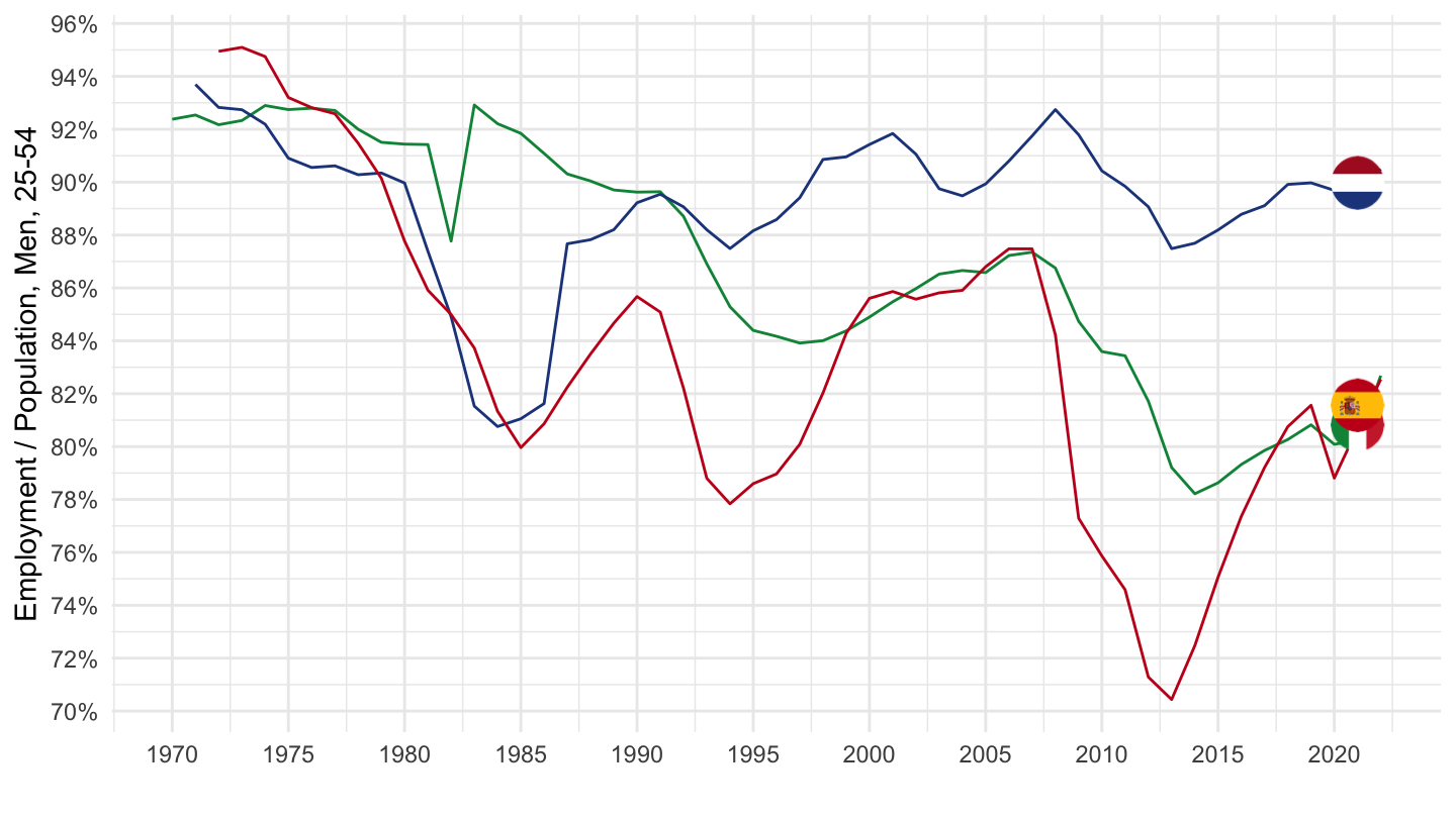
France, Norway, Portugal
Code
LFS_SEXAGE_I_R %>%
  filter(SERIES == "EPR",
         AGE == "2554",
         SEX == "MEN",
         COUNTRY %in% c("FRA", "NOR", "PRT")) %>%
  year_to_date %>%
  filter(date >= as.Date("1960-01-01")) %>%
  left_join(LFS_SEXAGE_I_R_var$COUNTRY, by = "COUNTRY") %>%
  select(Country, date, obsValue) %>%
  arrange(Country, date) %>%
  ggplot(.) + geom_line(aes(x = date, y = obsValue/100, color = Country)) +
  scale_color_manual(values = c("#002395", "#EF2B2D", "#006600")) +
  theme_minimal() + xlab("") + ylab("Employment / Population, Men, 25-54") +
  geom_image(data = . %>%
               filter(date == as.Date("2019-01-01")) %>%
               mutate(date = as.Date("2021-01-01"),
                      image = paste0("../../icon/flag/round/", str_to_lower(gsub(" ", "-", Country)), ".png")),
             aes(x = date, y = obsValue/100, image = image), asp = 1.5) +
  scale_x_date(breaks = seq(1960, 2100, 5) %>% paste0("-01-01") %>% as.Date,
               labels = date_format("%Y")) +
  theme(legend.position = "none") +
  scale_y_continuous(breaks = 0.01*seq(0, 200, 2),
                     labels = scales::percent_format(accuracy = 1))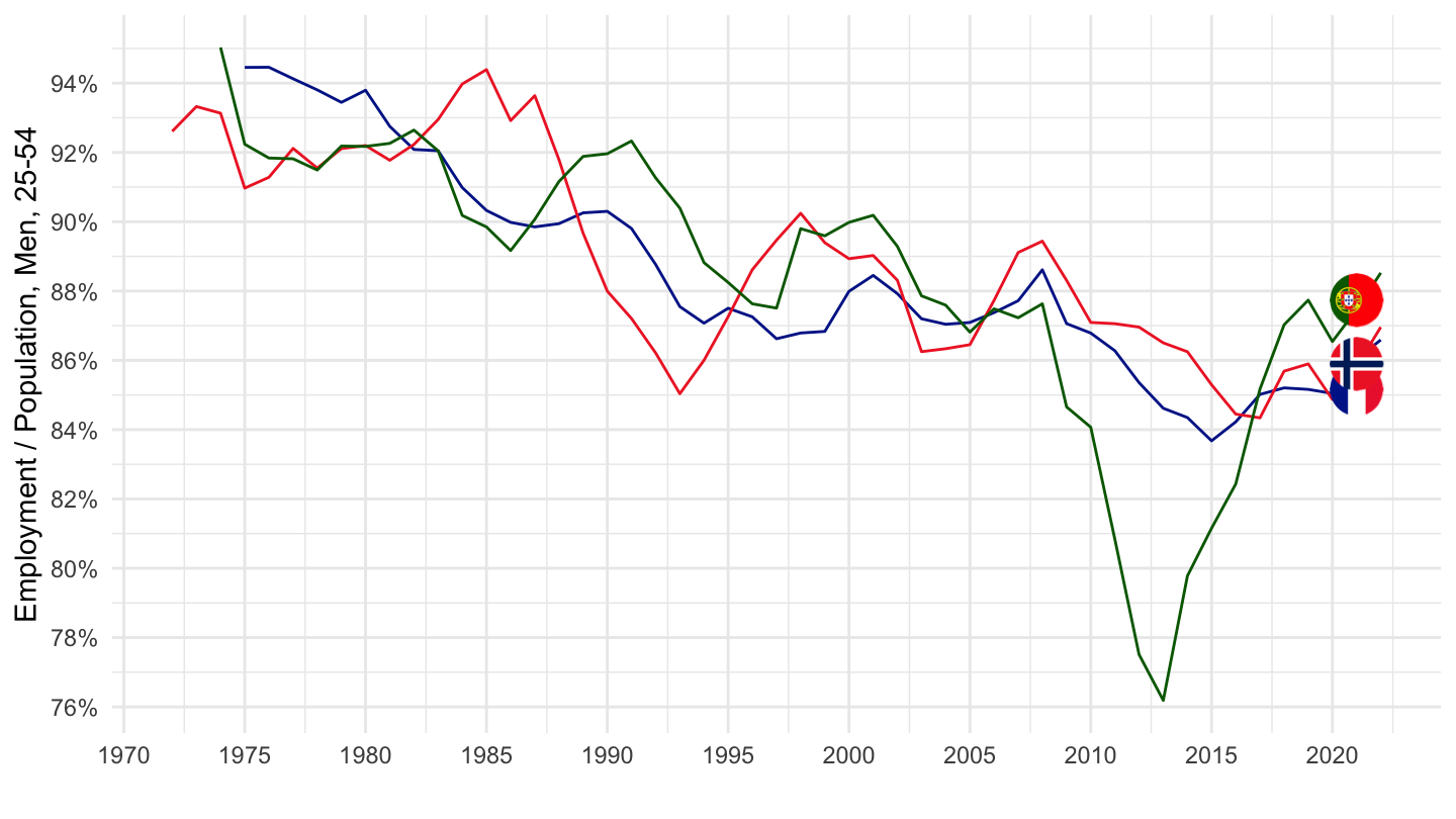
Belgium, Canada, Ireland, Korea
Code
LFS_SEXAGE_I_R %>%
  filter(SERIES == "EPR",
         AGE == "2554",
         SEX == "MEN",
         COUNTRY %in% c("BEL", "CAN", "IRL", "KOR")) %>%
  year_to_date %>%
  filter(date >= as.Date("1960-01-01")) %>%
  left_join(LFS_SEXAGE_I_R_var$COUNTRY, by = "COUNTRY") %>%
  select(Country, date, obsValue) %>%
  arrange(Country, date) %>%
  ggplot(.) + geom_line(aes(x = date, y = obsValue/100, color = Country)) +
  scale_color_manual(values = c("#000000", "#FF0000", "#FF883E", "#013478")) +
  theme_minimal() + xlab("") + ylab("Employment / Population, Men, 25-54") +
  geom_image(data = . %>%
               filter(date == as.Date("2019-01-01")) %>%
               mutate(date = as.Date("2021-01-01"),
                      image = paste0("../../icon/flag/round/", str_to_lower(gsub(" ", "-", Country)), ".png")),
             aes(x = date, y = obsValue/100, image = image), asp = 1.5) +
  scale_x_date(breaks = seq(1960, 2100, 5) %>% paste0("-01-01") %>% as.Date,
               labels = date_format("%Y")) +
  theme(legend.position = "none") +
  scale_y_continuous(breaks = 0.01*seq(0, 200, 2),
                     labels = scales::percent_format(accuracy = 1))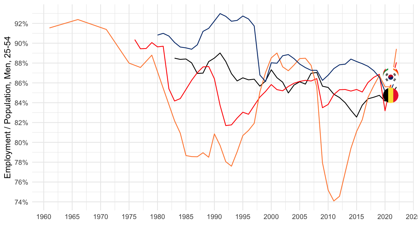
Europe, United States, United Kingdom
Employment Rate, 25-64, Men
Code
LFS_SEXAGE_I_R %>%
  filter(SERIES == "EPR",
         AGE == "2564",
         SEX == "MEN",
         COUNTRY %in% c("EUR", "GBR", "USA")) %>%
  year_to_date %>%
  filter(date >= as.Date("1980-01-01")) %>%
  left_join(LFS_SEXAGE_I_R_var$COUNTRY, by = "COUNTRY") %>%
  select(Country, date, obsValue) %>%
  arrange(Country, date) %>%
  ggplot(.) + geom_line(aes(x = date, y = obsValue/100, color = Country)) +
  scale_color_manual(values = c("#FFCC00", "#CF142B", "#3C3B6E")) +
  theme_minimal() + xlab("") + ylab("Employment / Population, Men, 25-54") +
  geom_image(data = . %>%
               filter(date == as.Date("2019-01-01")) %>%
               mutate(date = as.Date("2021-01-01"),
                      image = paste0("../../icon/flag/round/", str_to_lower(gsub(" ", "-", Country)), ".png")),
             aes(x = date, y = obsValue/100, image = image), asp = 1.5) +
  scale_x_date(breaks = seq(1960, 2100, 5) %>% paste0("-01-01") %>% as.Date,
               labels = date_format("%Y")) +
  theme(legend.position = "none") +
  scale_y_continuous(breaks = 0.01*seq(0, 200, 1),
                     labels = scales::percent_format(accuracy = 1))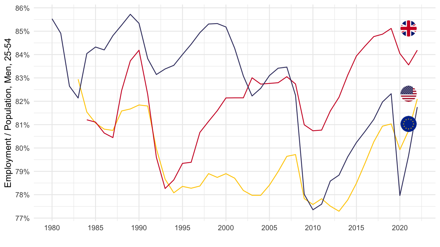
Employment Rate, 25-64, Men and Women
Code
LFS_SEXAGE_I_R %>%
  filter(SERIES == "EPR",
         AGE == "2564",
         SEX == "MW",
         COUNTRY %in% c("EUR", "GBR", "USA")) %>%
  year_to_date %>%
  filter(date >= as.Date("1980-01-01")) %>%
  left_join(LFS_SEXAGE_I_R_var$COUNTRY, by = "COUNTRY") %>%
  select(Country, date, obsValue) %>%
  arrange(Country, date) %>%
  ggplot(.) + geom_line(aes(x = date, y = obsValue/100, color = Country)) +
  scale_color_manual(values = c("#FFCC00", "#CF142B", "#3C3B6E")) +
  theme_minimal() + xlab("") + ylab("Employment / Population, Men, 25-54") +
  geom_image(data = . %>%
               filter(date == as.Date("2019-01-01")) %>%
               mutate(date = as.Date("2021-01-01"),
                      image = paste0("../../icon/flag/round/", str_to_lower(gsub(" ", "-", Country)), ".png")),
             aes(x = date, y = obsValue/100, image = image), asp = 1.5) +
  scale_x_date(breaks = seq(1960, 2100, 5) %>% paste0("-01-01") %>% as.Date,
               labels = date_format("%Y")) +
  theme(legend.position = "none") +
  scale_y_continuous(breaks = 0.01*seq(0, 200, 1),
                     labels = scales::percent_format(accuracy = 1))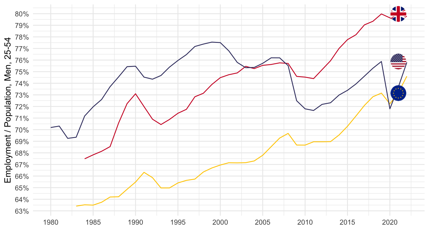
Unemployment Rate, 25-64, Men and Women
Code
LFS_SEXAGE_I_R %>%
  filter(SERIES == "UR",
         AGE == "2564",
         SEX == "MW",
         COUNTRY %in% c("EUR", "GBR", "USA")) %>%
  year_to_date %>%
  filter(date >= as.Date("1980-01-01")) %>%
  left_join(LFS_SEXAGE_I_R_var$COUNTRY, by = "COUNTRY") %>%
  select(Country, date, obsValue) %>%
  arrange(Country, date) %>%
  ggplot(.) + geom_line(aes(x = date, y = obsValue/100, color = Country)) +
  scale_color_manual(values = c("#FFCC00", "#CF142B", "#3C3B6E")) +
  theme_minimal() + xlab("") + ylab("") +
  geom_image(data = . %>%
               filter(date == as.Date("1997-01-01")) %>%
               mutate(date = as.Date("1997-01-01"),
                      image = paste0("../../icon/flag/round/", str_to_lower(gsub(" ", "-", Country)), ".png")),
             aes(x = date, y = obsValue/100, image = image), asp = 1.5) +
  scale_x_date(breaks = seq(1960, 2100, 5) %>% paste0("-01-01") %>% as.Date,
               labels = date_format("%Y")) +
  theme(legend.position = "none") +
  scale_y_continuous(breaks = 0.01*seq(0, 200, 1),
                     labels = scales::percent_format(accuracy = 1))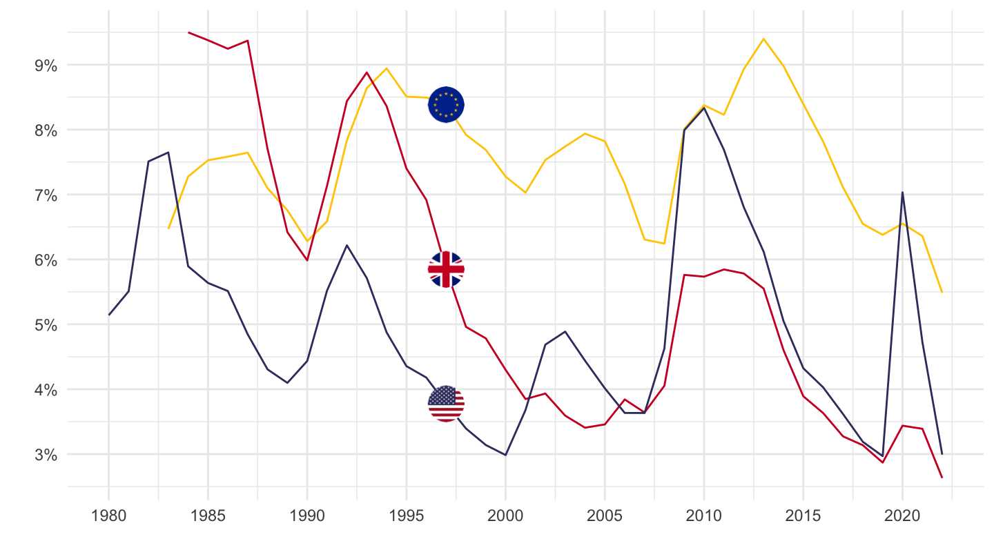
United States, Greece, Italy
Employment / Population ratio
All
Code
LFS_SEXAGE_I_R %>%
  filter(SERIES == "EPR",
         AGE == "1564",
         SEX == "MW",
         COUNTRY %in% c("USA", "GRC", "ITA")) %>%
  year_to_date %>%
  filter(date >= as.Date("1960-01-01")) %>%
  left_join(LFS_SEXAGE_I_R_var$COUNTRY, by = "COUNTRY") %>%
  select(Country, date, obsValue) %>%
  arrange(Country, date) %>%
  ggplot(.) + geom_line(aes(x = date, y = obsValue/100, color = Country)) +
  scale_color_manual(values = c("#0D5EAF", "#006600", "#C60B1E")) +
  theme_minimal() + xlab("") + ylab("Employment / Population") +
  geom_image(data = . %>%
               filter(date == as.Date("2019-01-01")) %>%
               mutate(date = as.Date("2021-01-01"),
                      image = paste0("../../icon/flag/round/", str_to_lower(gsub(" ", "-", Country)), ".png")),
             aes(x = date, y = obsValue/100, image = image), asp = 1.5) +
  scale_x_date(breaks = seq(1960, 2100, 5) %>% paste0("-01-01") %>% as.Date,
               labels = date_format("%Y")) +
  theme(legend.position = "none") +
  scale_y_continuous(breaks = 0.01*seq(0, 200, 5),
                     labels = scales::percent_format(accuracy = 1))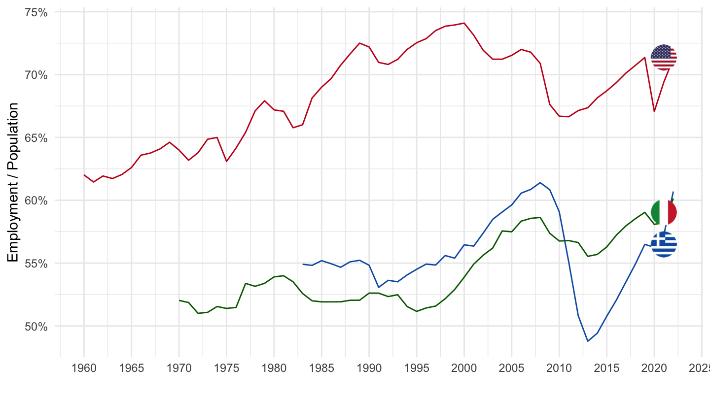
Greece, Portugal, Spain
Employment / Population ratio
All
Code
LFS_SEXAGE_I_R %>%
  filter(SERIES == "EPR",
         AGE == "1564",
         SEX == "MW",
         COUNTRY %in% c("GRC", "PRT", "ESP")) %>%
  year_to_date %>%
  filter(date >= as.Date("1960-01-01")) %>%
  left_join(LFS_SEXAGE_I_R_var$COUNTRY, by = "COUNTRY") %>%
  select(Country, date, obsValue) %>%
  arrange(Country, date) %>%
  ggplot(.) + geom_line(aes(x = date, y = obsValue/100, color = Country)) +
  scale_color_manual(values = c("#0D5EAF", "#006600", "#C60B1E")) +
  theme_minimal() + xlab("") + ylab("") +
  geom_image(data = . %>%
               filter(date == as.Date("2019-01-01")) %>%
               mutate(date = as.Date("2021-01-01"),
                      image = paste0("../../icon/flag/round/", str_to_lower(Country), ".png")),
             aes(x = date, y = obsValue/100, image = image), asp = 1.5) +
  scale_x_date(breaks = seq(1960, 2100, 5) %>% paste0("-01-01") %>% as.Date,
               labels = date_format("%Y")) +
  theme(legend.position = "none") +
  scale_y_continuous(breaks = 0.01*seq(0, 200, 5),
                     labels = scales::percent_format(accuracy = 1))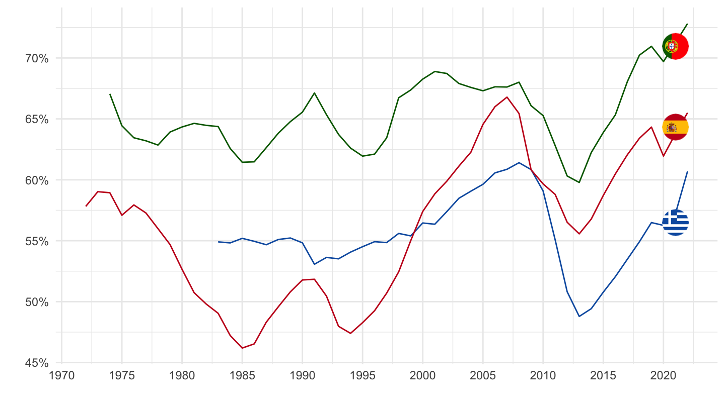
Men
Code
LFS_SEXAGE_I_R %>%
  filter(SERIES == "EPR",
         AGE == "1564",
         SEX == "MEN",
         COUNTRY %in% c("GRC", "PRT", "ESP")) %>%
  year_to_date %>%
  filter(date >= as.Date("1960-01-01")) %>%
  left_join(LFS_SEXAGE_I_R_var$COUNTRY, by = "COUNTRY") %>%
  select(Country, date, obsValue) %>%
  arrange(Country, date) %>%
  ggplot(.) + geom_line(aes(x = date, y = obsValue/100, color = Country)) +
  scale_color_manual(values = c("#0D5EAF", "#006600", "#C60B1E")) +
  theme_minimal() + xlab("") + ylab("") +
  geom_image(data = . %>%
               filter(date == as.Date("2019-01-01")) %>%
               mutate(date = as.Date("2021-01-01"),
                      image = paste0("../../icon/flag/round/", str_to_lower(Country), ".png")),
             aes(x = date, y = obsValue/100, image = image), asp = 1.5) +
  scale_x_date(breaks = seq(1960, 2100, 5) %>% paste0("-01-01") %>% as.Date,
               labels = date_format("%Y")) +
  theme(legend.position = "none") +
  scale_y_continuous(breaks = 0.01*seq(0, 200, 5),
                     labels = scales::percent_format(accuracy = 1))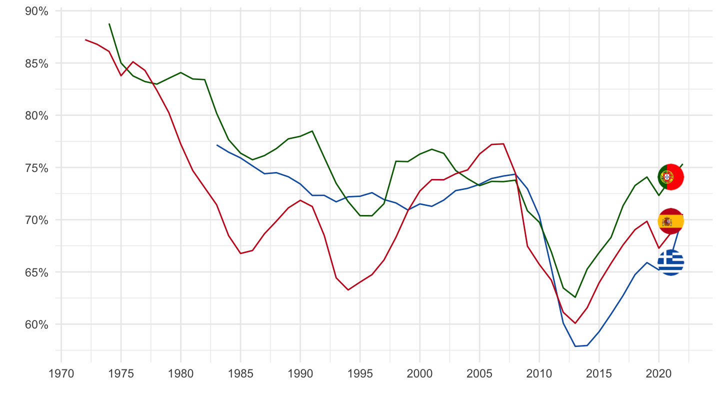
Women
Code
LFS_SEXAGE_I_R %>%
  filter(SERIES == "EPR",
         AGE == "1564",
         SEX == "WOMEN",
         COUNTRY %in% c("GRC", "PRT", "ESP")) %>%
  year_to_date %>%
  filter(date >= as.Date("1960-01-01")) %>%
  left_join(LFS_SEXAGE_I_R_var$COUNTRY, by = "COUNTRY") %>%
  select(Country, date, obsValue) %>%
  arrange(Country, date) %>%
  ggplot(.) + geom_line(aes(x = date, y = obsValue/100, color = Country)) +
  scale_color_manual(values = c("#0D5EAF", "#006600", "#C60B1E")) +
  theme_minimal() + xlab("") + ylab("") +
  geom_image(data = . %>%
               filter(date == as.Date("2019-01-01")) %>%
               mutate(date = as.Date("2021-01-01"),
                      image = paste0("../../icon/flag/round/", str_to_lower(Country), ".png")),
             aes(x = date, y = obsValue/100, image = image), asp = 1.5) +
  scale_x_date(breaks = seq(1960, 2100, 5) %>% paste0("-01-01") %>% as.Date,
               labels = date_format("%Y")) +
  theme(legend.position = "none") +
  scale_y_continuous(breaks = 0.01*seq(0, 200, 5),
                     labels = scales::percent_format(accuracy = 1))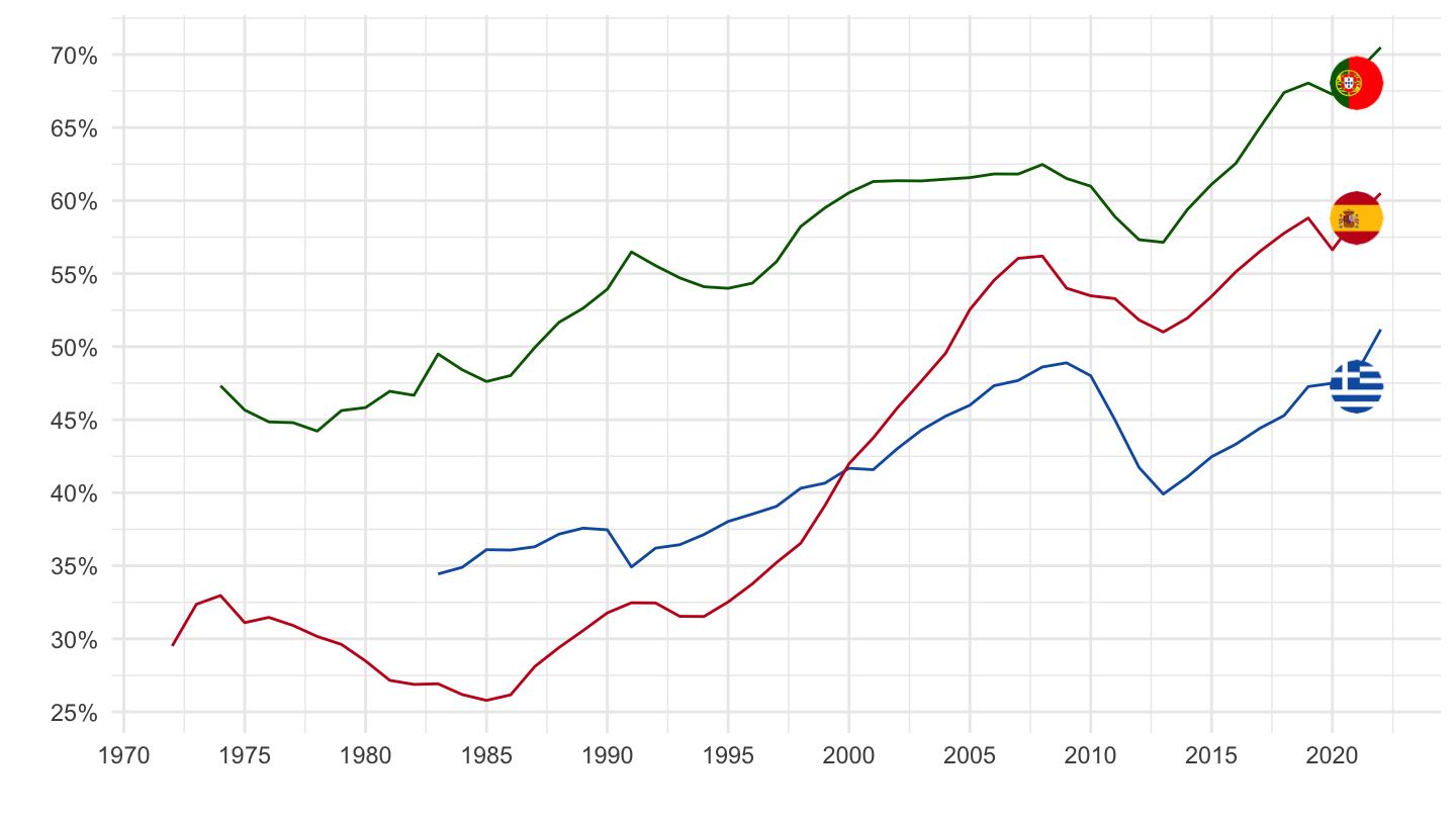
Unemployment Rate
Code
LFS_SEXAGE_I_R %>%
  filter(SERIES == "UR",
         AGE == "1564",
         SEX == "MW",
         COUNTRY %in% c("GRC", "PRT", "ESP")) %>%
  year_to_date %>%
  filter(date >= as.Date("1960-01-01")) %>%
  left_join(LFS_SEXAGE_I_R_var$COUNTRY, by = "COUNTRY") %>%
  select(Country, date, obsValue) %>%
  arrange(Country, date) %>%
  ggplot(.) + geom_line(aes(x = date, y = obsValue/100, color = Country)) +
  scale_color_manual(values = c("#0D5EAF", "#006600", "#C60B1E")) +
  theme_minimal() + xlab("") + ylab("") +
  geom_image(data = . %>%
               filter(date == as.Date("2019-01-01")) %>%
               mutate(date = as.Date("2021-01-01"),
                      image = paste0("../../icon/flag/round/", str_to_lower(Country), ".png")),
             aes(x = date, y = obsValue/100, image = image), asp = 1.5) +
  scale_x_date(breaks = seq(1960, 2100, 5) %>% paste0("-01-01") %>% as.Date,
               labels = date_format("%Y")) +
  theme(legend.position = "none") +
  scale_y_continuous(breaks = 0.01*seq(0, 200, 1),
                     labels = scales::percent_format(accuracy = 1))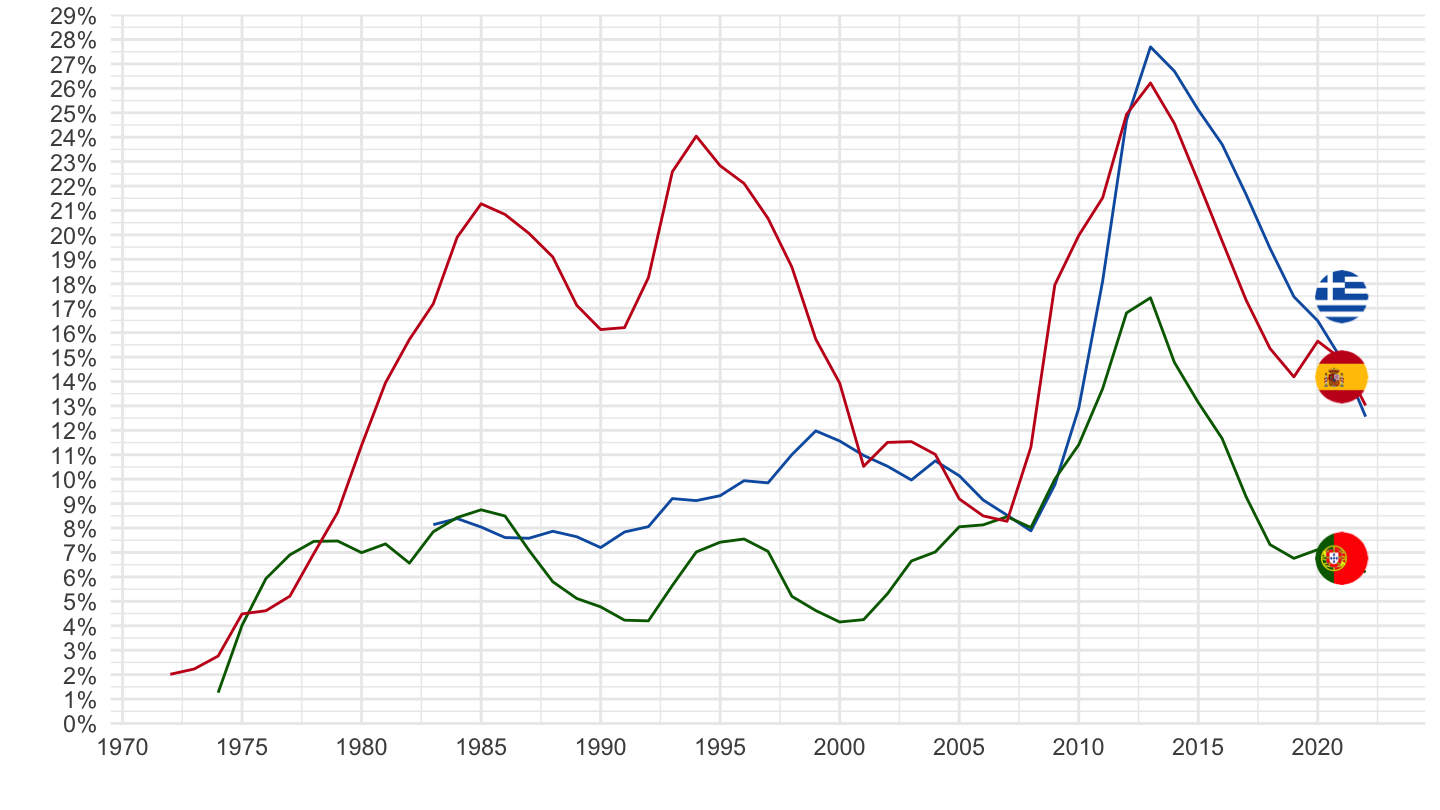
Labour force participation rate - LFPR
Code
LFS_SEXAGE_I_R %>%
  filter(SERIES == "LFPR",
         AGE == "1564",
         SEX == "MW",
         COUNTRY %in% c("GRC", "PRT", "ESP")) %>%
  year_to_date %>%
  filter(date >= as.Date("1960-01-01")) %>%
  left_join(LFS_SEXAGE_I_R_var$COUNTRY, by = "COUNTRY") %>%
  select(Country, date, obsValue) %>%
  arrange(Country, date) %>%
  ggplot(.) + geom_line(aes(x = date, y = obsValue/100, color = Country)) +
  scale_color_manual(values = c("#0D5EAF", "#006600", "#C60B1E")) +
  theme_minimal() + xlab("") + ylab("") +
  geom_image(data = . %>%
               filter(date == as.Date("2019-01-01")) %>%
               mutate(date = as.Date("2021-01-01"),
                      image = paste0("../../icon/flag/round/", str_to_lower(Country), ".png")),
             aes(x = date, y = obsValue/100, image = image), asp = 1.5) +
  scale_x_date(breaks = seq(1960, 2100, 5) %>% paste0("-01-01") %>% as.Date,
               labels = date_format("%Y")) +
  theme(legend.position = "none") +
  scale_y_continuous(breaks = 0.01*seq(0, 200, 5),
                     labels = scales::percent_format(accuracy = 1))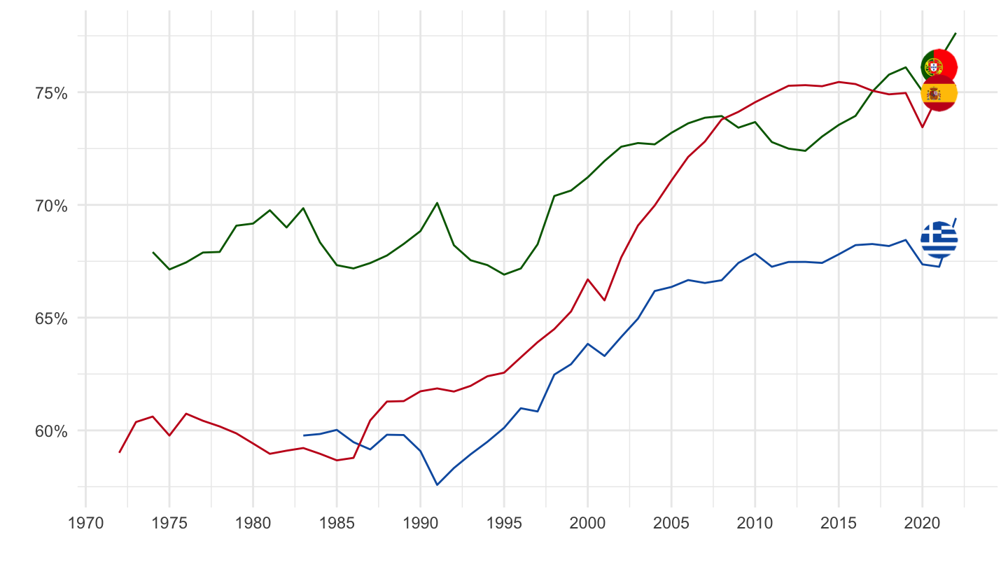
Germany, France, Italy
Employment / Population ratio
All
Code
LFS_SEXAGE_I_R %>%
  filter(SERIES == "EPR",
         AGE == "1564",
         SEX == "MW",
         COUNTRY %in% c("ITA", "DEU", "FRA")) %>%
  year_to_date %>%
  filter(date >= as.Date("1960-01-01")) %>%
  left_join(LFS_SEXAGE_I_R_var$COUNTRY, by = "COUNTRY") %>%
  select(Country, date, obsValue) %>%
  arrange(Country, date) %>%
  ggplot(.) + geom_line(aes(x = date, y = obsValue/100, color = Country)) +
  scale_color_manual(values = c("#002395", "#000000", "#009246")) +
  theme_minimal() + xlab("") + ylab("") +
  geom_image(data = . %>%
               filter(date == as.Date("2019-01-01")) %>%
               mutate(date = as.Date("2021-01-01"),
                      image = paste0("../../icon/flag/round/", str_to_lower(Country), ".png")),
             aes(x = date, y = obsValue/100, image = image), asp = 1.5) +
  scale_x_date(breaks = seq(1960, 2100, 5) %>% paste0("-01-01") %>% as.Date,
               labels = date_format("%Y")) +
  theme(legend.position = "none") +
  scale_y_continuous(breaks = 0.01*seq(0, 200, 5),
                     labels = scales::percent_format(accuracy = 1))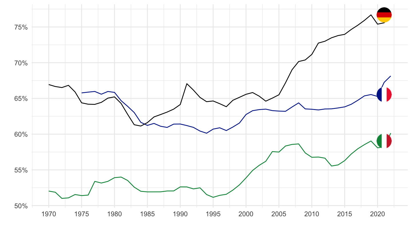
Men
15-64
Code
LFS_SEXAGE_I_R %>%
  filter(SERIES == "EPR",
         AGE == "1564",
         SEX == "MEN",
         COUNTRY %in% c("ITA", "DEU", "FRA")) %>%
  year_to_date %>%
  filter(date >= as.Date("1960-01-01")) %>%
  left_join(LFS_SEXAGE_I_R_var$COUNTRY, by = "COUNTRY") %>%
  select(Country, date, obsValue) %>%
  arrange(Country, date) %>%
  ggplot(.) + geom_line(aes(x = date, y = obsValue/100, color = Country)) +
  scale_color_manual(values = c("#002395", "#000000", "#009246")) +
  theme_minimal() + xlab("") + ylab("") +
  geom_image(data = . %>%
               filter(date == as.Date("2019-01-01")) %>%
               mutate(date = as.Date("2021-01-01"),
                      image = paste0("../../icon/flag/round/", str_to_lower(Country), ".png")),
             aes(x = date, y = obsValue/100, image = image), asp = 1.5) +
  scale_x_date(breaks = seq(1960, 2100, 5) %>% paste0("-01-01") %>% as.Date,
               labels = date_format("%Y")) +
  theme(legend.position = "none") +
  scale_y_continuous(breaks = 0.01*seq(0, 200, 5),
                     labels = scales::percent_format(accuracy = 1))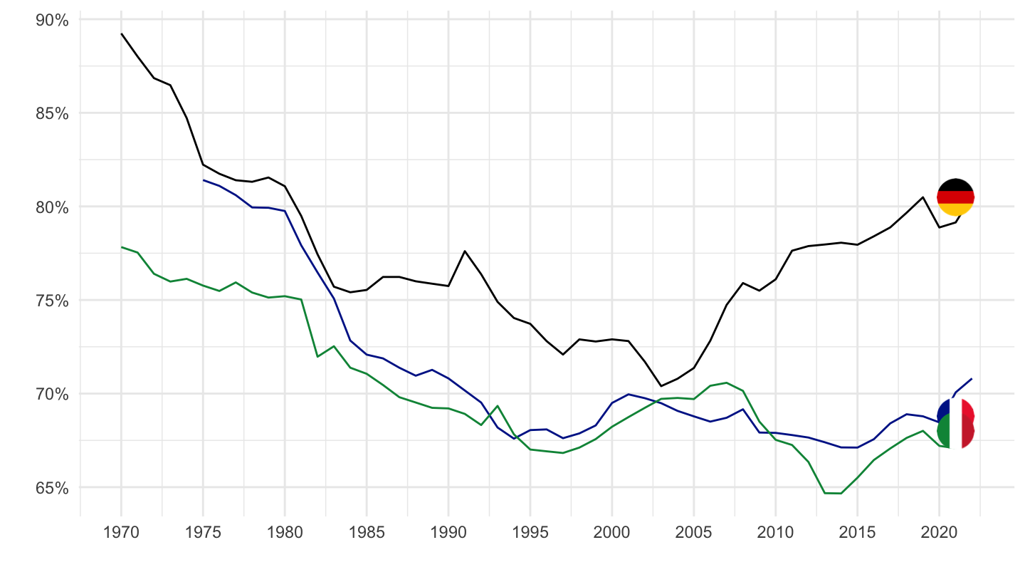
25-64
Code
LFS_SEXAGE_I_R %>%
  filter(SERIES == "EPR",
         AGE == "2564",
         SEX == "MEN",
         COUNTRY %in% c("ITA", "DEU", "FRA")) %>%
  year_to_date %>%
  filter(date >= as.Date("1960-01-01")) %>%
  left_join(LFS_SEXAGE_I_R_var$COUNTRY, by = "COUNTRY") %>%
  select(Country, date, obsValue) %>%
  arrange(Country, date) %>%
  ggplot(.) + geom_line(aes(x = date, y = obsValue/100, color = Country)) +
  scale_color_manual(values = c("#002395", "#000000", "#009246")) +
  theme_minimal() + xlab("") + ylab("") +
  geom_image(data = . %>%
               filter(date == as.Date("2019-01-01")) %>%
               mutate(date = as.Date("2021-01-01"),
                      image = paste0("../../icon/flag/round/", str_to_lower(Country), ".png")),
             aes(x = date, y = obsValue/100, image = image), asp = 1.5) +
  scale_x_date(breaks = seq(1960, 2100, 5) %>% paste0("-01-01") %>% as.Date,
               labels = date_format("%Y")) +
  theme(legend.position = "none") +
  scale_y_continuous(breaks = 0.01*seq(0, 200, 5),
                     labels = scales::percent_format(accuracy = 1))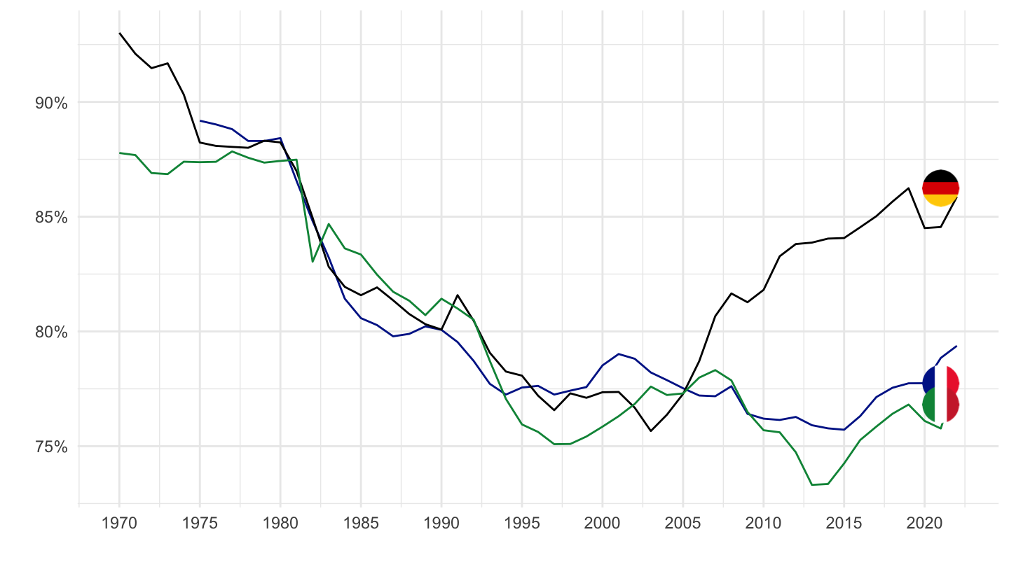
Women
15-64
Code
LFS_SEXAGE_I_R %>%
  filter(SERIES == "EPR",
         AGE == "1564",
         SEX == "WOMEN",
         COUNTRY %in% c("ITA", "DEU", "FRA")) %>%
  year_to_date %>%
  filter(date >= as.Date("1960-01-01")) %>%
  left_join(LFS_SEXAGE_I_R_var$COUNTRY, by = "COUNTRY") %>%
  select(Country, date, obsValue) %>%
  arrange(Country, date) %>%
  ggplot(.) + geom_line(aes(x = date, y = obsValue/100, color = Country)) +
  scale_color_manual(values = c("#002395", "#000000", "#009246")) +
  theme_minimal() + xlab("") + ylab("") +
  geom_image(data = . %>%
               filter(date == as.Date("2019-01-01")) %>%
               mutate(date = as.Date("2021-01-01"),
                      image = paste0("../../icon/flag/round/", str_to_lower(Country), ".png")),
             aes(x = date, y = obsValue/100, image = image), asp = 1.5) +
  scale_x_date(breaks = seq(1960, 2100, 5) %>% paste0("-01-01") %>% as.Date,
               labels = date_format("%Y")) +
  theme(legend.position = "none") +
  scale_y_continuous(breaks = 0.01*seq(0, 200, 5),
                     labels = scales::percent_format(accuracy = 1))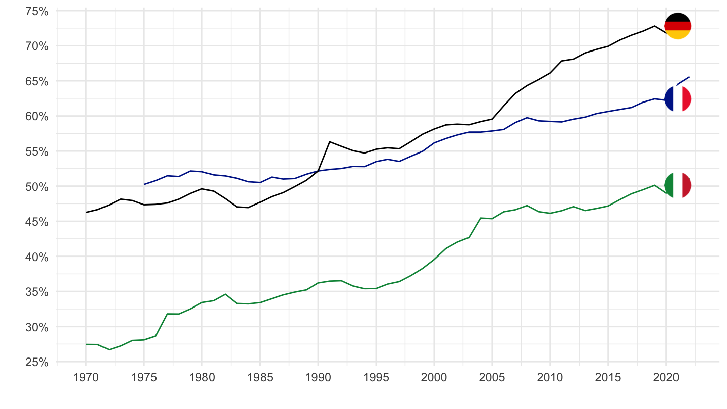
25-64
Code
LFS_SEXAGE_I_R %>%
  filter(SERIES == "EPR",
         AGE == "2564",
         SEX == "WOMEN",
         COUNTRY %in% c("ITA", "DEU", "FRA")) %>%
  year_to_date %>%
  filter(date >= as.Date("1960-01-01")) %>%
  left_join(LFS_SEXAGE_I_R_var$COUNTRY, by = "COUNTRY") %>%
  select(Country, date, obsValue) %>%
  arrange(Country, date) %>%
  ggplot(.) + geom_line(aes(x = date, y = obsValue/100, color = Country)) +
  scale_color_manual(values = c("#002395", "#000000", "#009246")) +
  theme_minimal() + xlab("") + ylab("") +
  geom_image(data = . %>%
               filter(date == as.Date("2019-01-01")) %>%
               mutate(date = as.Date("2021-01-01"),
                      image = paste0("../../icon/flag/round/", str_to_lower(Country), ".png")),
             aes(x = date, y = obsValue/100, image = image), asp = 1.5) +
  scale_x_date(breaks = seq(1960, 2100, 5) %>% paste0("-01-01") %>% as.Date,
               labels = date_format("%Y")) +
  theme(legend.position = "none") +
  scale_y_continuous(breaks = 0.01*seq(0, 200, 5),
                     labels = scales::percent_format(accuracy = 1))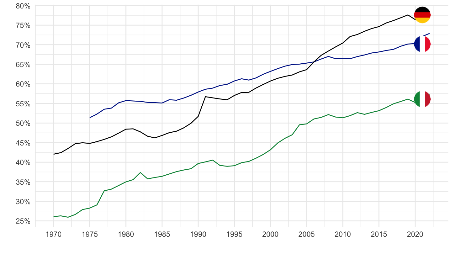
25-54
Code
LFS_SEXAGE_I_R %>%
  filter(SERIES == "EPR",
         AGE == "2554",
         SEX == "WOMEN",
         COUNTRY %in% c("ITA", "DEU", "FRA")) %>%
  year_to_date %>%
  filter(date >= as.Date("1960-01-01")) %>%
  left_join(LFS_SEXAGE_I_R_var$COUNTRY, by = "COUNTRY") %>%
  select(Country, date, obsValue) %>%
  arrange(Country, date) %>%
  ggplot(.) + geom_line(aes(x = date, y = obsValue/100, color = Country)) +
  scale_color_manual(values = c("#002395", "#000000", "#009246")) +
  theme_minimal() + xlab("") + ylab("") +
  geom_image(data = . %>%
               filter(date == as.Date("2019-01-01")) %>%
               mutate(date = as.Date("2021-01-01"),
                      image = paste0("../../icon/flag/round/", str_to_lower(Country), ".png")),
             aes(x = date, y = obsValue/100, image = image), asp = 1.5) +
  scale_x_date(breaks = seq(1960, 2100, 5) %>% paste0("-01-01") %>% as.Date,
               labels = date_format("%Y")) +
  theme(legend.position = "none") +
  scale_y_continuous(breaks = 0.01*seq(0, 200, 5),
                     labels = scales::percent_format(accuracy = 1))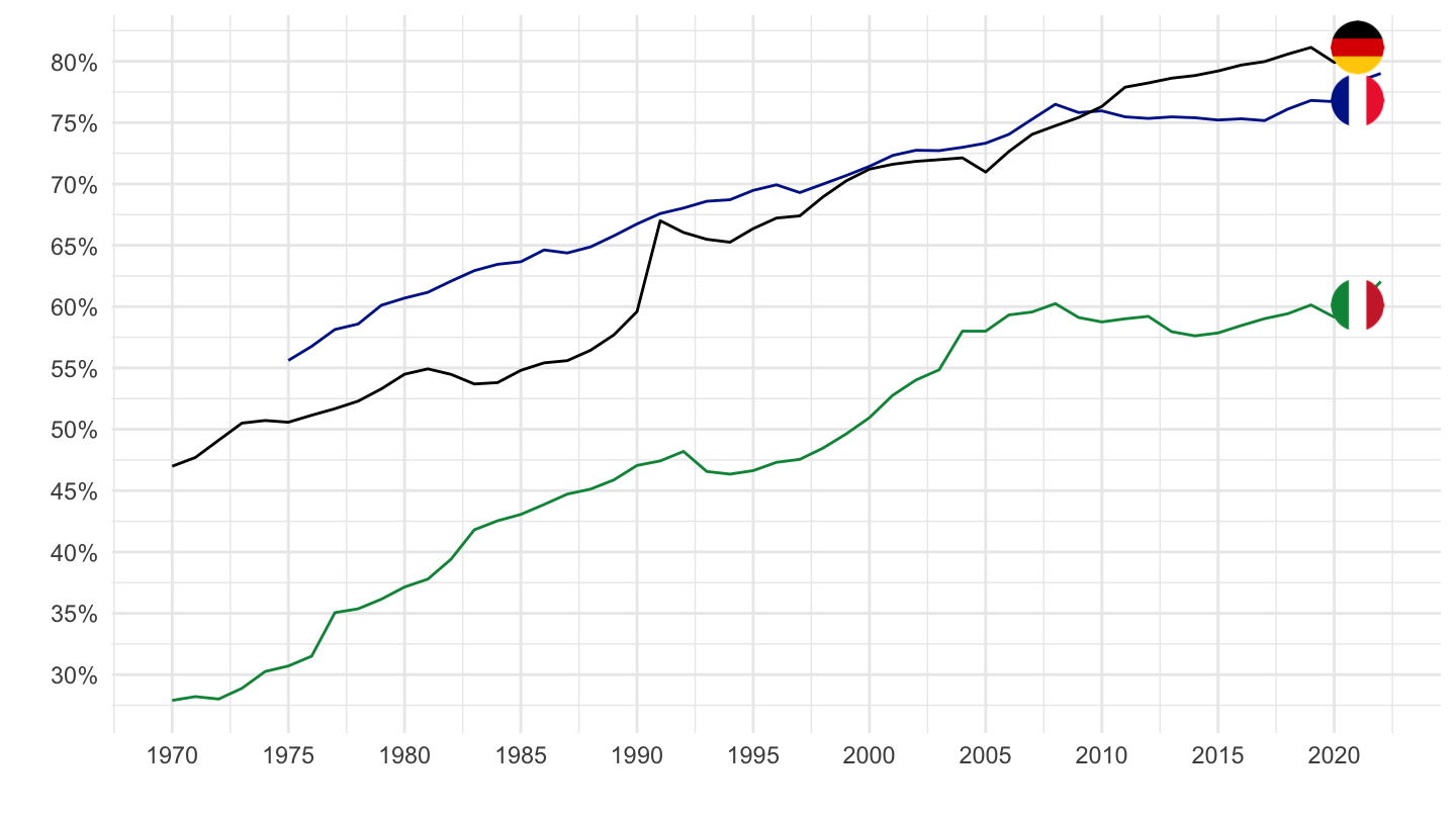
Unemployment Rate
All
Code
LFS_SEXAGE_I_R %>%
  filter(SERIES == "UR",
         AGE == "1564",
         SEX == "MW",
         COUNTRY %in% c("ITA", "DEU", "FRA")) %>%
  year_to_date %>%
  filter(date >= as.Date("1960-01-01")) %>%
  left_join(LFS_SEXAGE_I_R_var$COUNTRY, by = "COUNTRY") %>%
  select(Country, date, obsValue) %>%
  arrange(Country, date) %>%
  ggplot(.) + geom_line(aes(x = date, y = obsValue/100, color = Country)) +
  scale_color_manual(values = c("#002395", "#000000", "#009246")) +
  theme_minimal() + xlab("") + ylab("") +
  geom_image(data = . %>%
               filter(date == as.Date("2019-01-01")) %>%
               mutate(date = as.Date("2021-01-01"),
                      image = paste0("../../icon/flag/round/", str_to_lower(Country), ".png")),
             aes(x = date, y = obsValue/100, image = image), asp = 1.5) +
  scale_x_date(breaks = seq(1960, 2100, 5) %>% paste0("-01-01") %>% as.Date,
               labels = date_format("%Y")) +
  theme(legend.position = "none") +
  scale_y_continuous(breaks = 0.01*seq(0, 200, 1),
                     labels = scales::percent_format(accuracy = 1))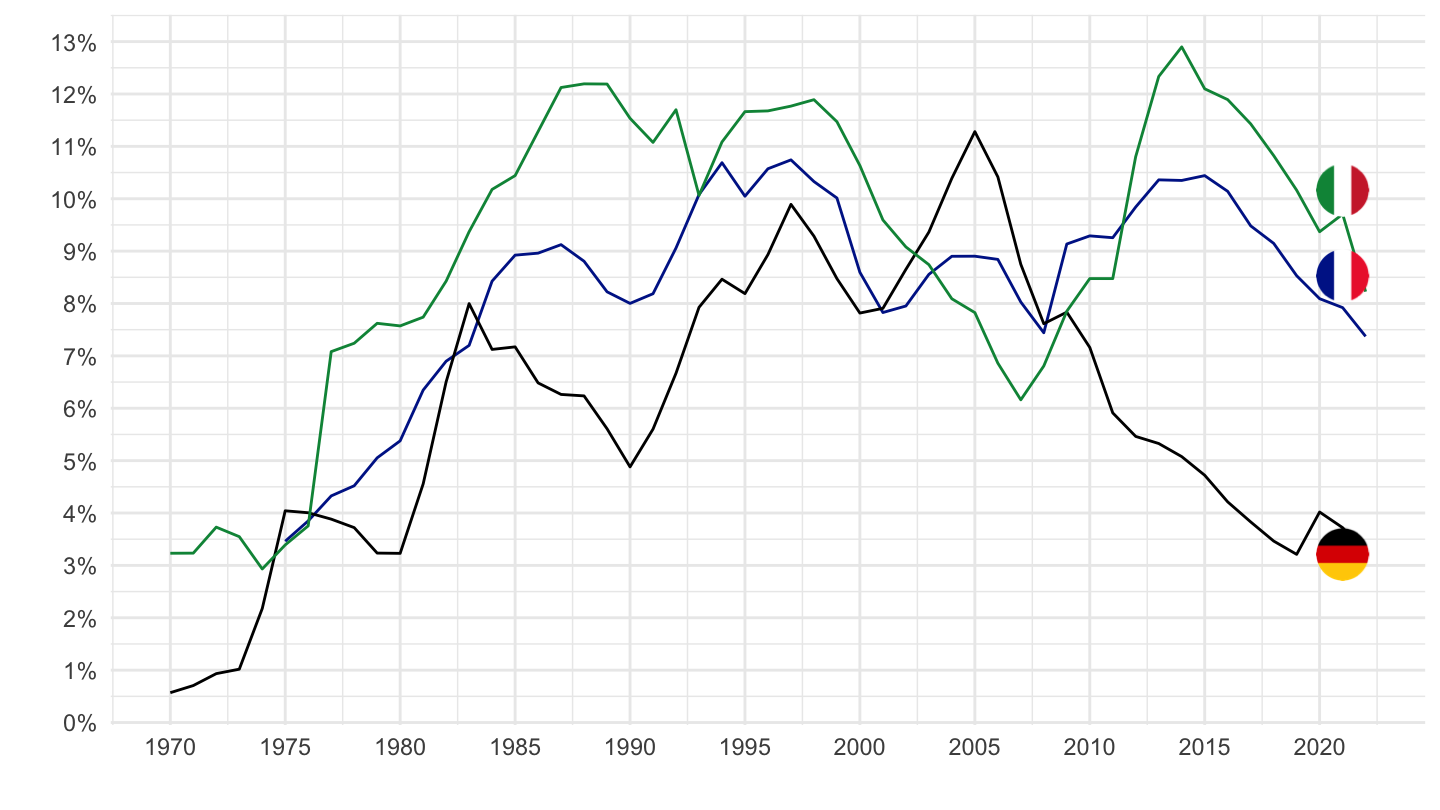
Labour force participation rate - LFPR
All
Code
LFS_SEXAGE_I_R %>%
  filter(SERIES == "LFPR",
         AGE == "1564",
         SEX == "MW",
         COUNTRY %in% c("ITA", "DEU", "FRA")) %>%
  year_to_date %>%
  filter(date >= as.Date("1960-01-01")) %>%
  left_join(LFS_SEXAGE_I_R_var$COUNTRY, by = "COUNTRY") %>%
  select(Country, date, obsValue) %>%
  arrange(Country, date) %>%
  ggplot(.) + geom_line(aes(x = date, y = obsValue/100, color = Country)) +
  scale_color_manual(values = c("#002395", "#000000", "#009246")) +
  theme_minimal() + xlab("") + ylab("") +
  geom_image(data = . %>%
               filter(date == as.Date("2019-01-01")) %>%
               mutate(date = as.Date("2021-01-01"),
                      image = paste0("../../icon/flag/round/", str_to_lower(Country), ".png")),
             aes(x = date, y = obsValue/100, image = image), asp = 1.5) +
  scale_x_date(breaks = seq(1960, 2100, 5) %>% paste0("-01-01") %>% as.Date,
               labels = date_format("%Y")) +
  theme(legend.position = "none") +
  scale_y_continuous(breaks = 0.01*seq(0, 200, 5),
                     labels = scales::percent_format(accuracy = 1))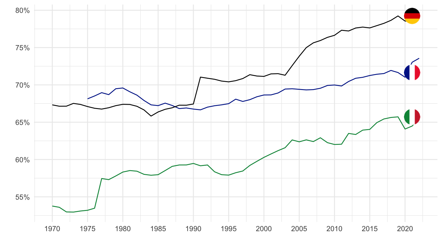
Men
Code
LFS_SEXAGE_I_R %>%
  filter(SERIES == "LFPR",
         AGE == "1564",
         SEX == "MEN",
         COUNTRY %in% c("ITA", "DEU", "FRA")) %>%
  year_to_date %>%
  filter(date >= as.Date("1960-01-01")) %>%
  left_join(LFS_SEXAGE_I_R_var$COUNTRY, by = "COUNTRY") %>%
  select(Country, date, obsValue) %>%
  arrange(Country, date) %>%
  ggplot(.) + geom_line(aes(x = date, y = obsValue/100, color = Country)) +
  scale_color_manual(values = c("#002395", "#000000", "#009246")) +
  theme_minimal() + xlab("") + ylab("") +
  geom_image(data = . %>%
               filter(date == as.Date("2019-01-01")) %>%
               mutate(date = as.Date("2021-01-01"),
                      image = paste0("../../icon/flag/round/", str_to_lower(Country), ".png")),
             aes(x = date, y = obsValue/100, image = image), asp = 1.5) +
  scale_x_date(breaks = seq(1960, 2100, 5) %>% paste0("-01-01") %>% as.Date,
               labels = date_format("%Y")) +
  theme(legend.position = "none") +
  scale_y_continuous(breaks = 0.01*seq(0, 200, 5),
                     labels = scales::percent_format(accuracy = 1))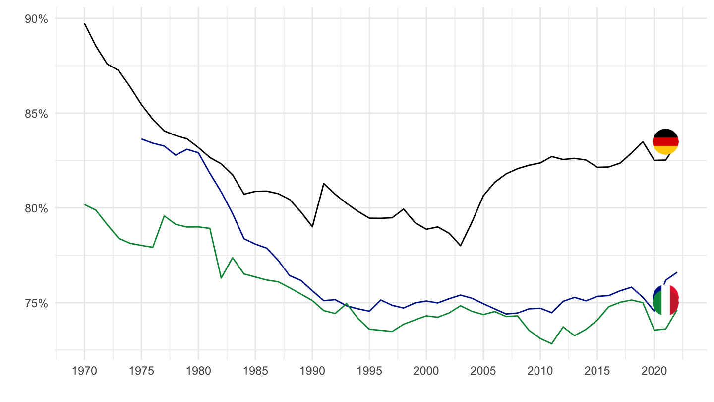
Italy, Germany, Greece, Spain, Portugal, France
EP - All
FLAGS
2000-
Code
LFS_SEXAGE_I_R %>%
  filter(SERIES == "EPR",
         AGE == "1564",
         SEX == "MW",
         COUNTRY %in% c("ITA", "DEU", "GRC", "ESP", "PRT", "FRA")) %>%
  year_to_date %>%
  filter(date >= as.Date("2000-01-01")) %>%
  left_join(LFS_SEXAGE_I_R_var$COUNTRY, by = "COUNTRY") %>%
  select(Country, date, obsValue) %>%
  arrange(Country, date) %>%
  ggplot(.) + geom_line(aes(x = date, y = obsValue/100, color = Country)) +
  scale_color_manual(values = c("#002395", "#000000", "#0D5EAF",
                                "#CE2B37", "#006600", "#FFC400")) +
  theme_minimal() + xlab("") + ylab("") +
  geom_image(data = . %>%
               filter(date == as.Date("2019-01-01")) %>%
               mutate(date = as.Date("2020-01-01"),
                      image = paste0("../../icon/flag/round/", str_to_lower(Country), ".png")),
             aes(x = date, y = obsValue/100, image = image), asp = 1.5) +
  scale_x_date(breaks = seq(1960, 2100, 1) %>% paste0("-01-01") %>% as.Date,
               labels = date_format("%Y")) +
  theme(legend.position = "none") +
  scale_y_continuous(breaks = 0.01*seq(0, 200, 5),
                     labels = scales::percent_format(accuracy = 1))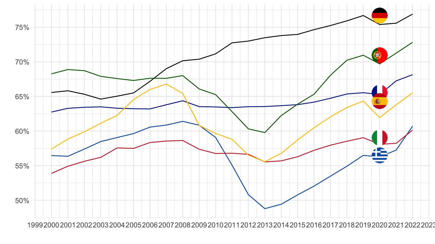
1990-
Code
LFS_SEXAGE_I_R %>%
  filter(SERIES == "EPR",
         AGE == "1564",
         SEX == "MW",
         COUNTRY %in% c("ITA", "DEU", "GRC", "ESP", "PRT", "FRA")) %>%
  year_to_date %>%
  filter(date >= as.Date("1990-01-01")) %>%
  left_join(LFS_SEXAGE_I_R_var$COUNTRY, by = "COUNTRY") %>%
  select(Country, date, obsValue) %>%
  arrange(Country, date) %>%
  ggplot(.) + geom_line(aes(x = date, y = obsValue/100, color = Country)) +
  scale_color_manual(values = c("#002395", "#000000", "#0D5EAF",
                                "#CE2B37", "#006600", "#FFC400")) +
  theme_minimal() + xlab("") + ylab("") +
  geom_image(data = . %>%
               filter(date == as.Date("2019-01-01")) %>%
               mutate(date = as.Date("2020-01-01"),
                      image = paste0("../../icon/flag/round/", str_to_lower(Country), ".png")),
             aes(x = date, y = obsValue/100, image = image), asp = 1.5) +
  scale_x_date(breaks = seq(1960, 2100, 5) %>% paste0("-01-01") %>% as.Date,
               labels = date_format("%Y")) +
  theme(legend.position = "none") +
  scale_y_continuous(breaks = 0.01*seq(0, 200, 5),
                     labels = scales::percent_format(accuracy = 1))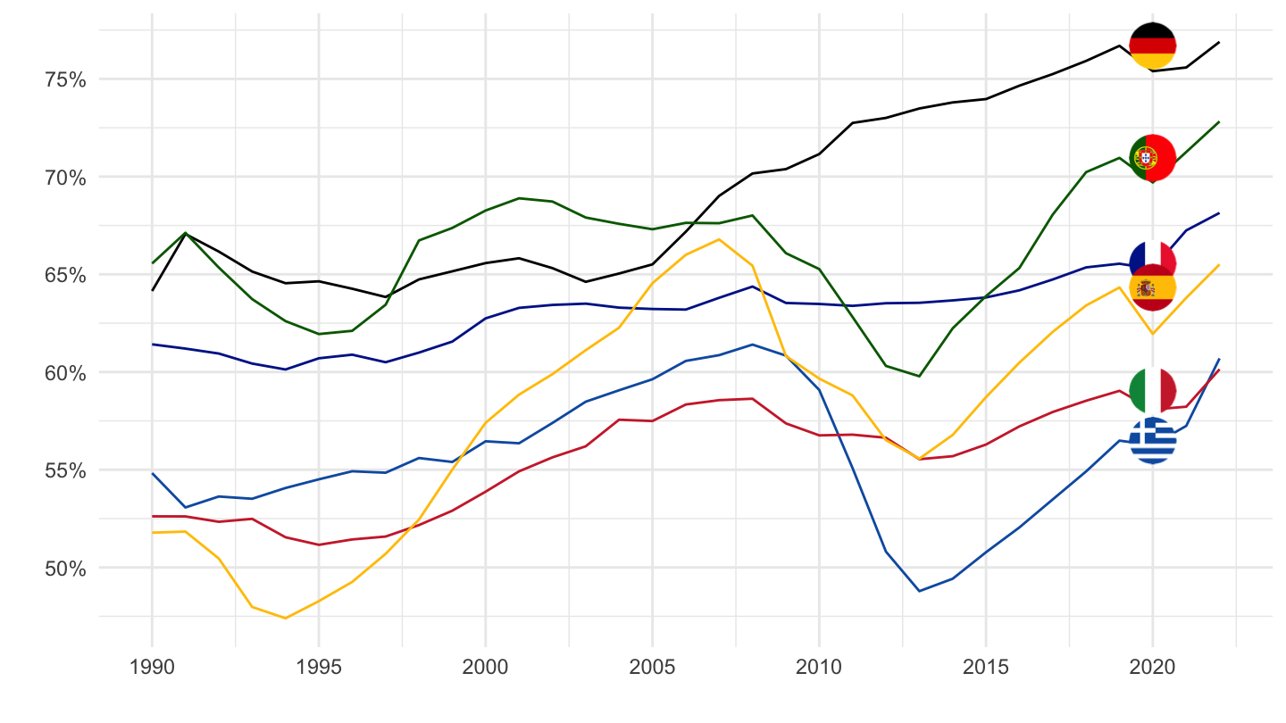
1980-
Code
LFS_SEXAGE_I_R %>%
  filter(SERIES == "EPR",
         AGE == "1564",
         SEX == "MW",
         COUNTRY %in% c("ITA", "DEU", "GRC", "ESP", "PRT", "FRA")) %>%
  year_to_date %>%
  filter(date >= as.Date("1980-01-01")) %>%
  left_join(LFS_SEXAGE_I_R_var$COUNTRY, by = "COUNTRY") %>%
  select(Country, date, obsValue) %>%
  arrange(Country, date) %>%
  ggplot(.) + geom_line(aes(x = date, y = obsValue/100, color = Country)) +
  scale_color_manual(values = c("#002395", "#000000", "#0D5EAF",
                                "#CE2B37", "#006600", "#FFC400")) +
  theme_minimal() + xlab("") + ylab("") +
  geom_image(data = . %>%
               filter(date == as.Date("2019-01-01")) %>%
               mutate(date = as.Date("2020-01-01"),
                      image = paste0("../../icon/flag/round/", str_to_lower(Country), ".png")),
             aes(x = date, y = obsValue/100, image = image), asp = 1.5) +
  scale_x_date(breaks = seq(1960, 2100, 5) %>% paste0("-01-01") %>% as.Date,
               labels = date_format("%Y")) +
  theme(legend.position = "none") +
  scale_y_continuous(breaks = 0.01*seq(0, 200, 5),
                     labels = scales::percent_format(accuracy = 1))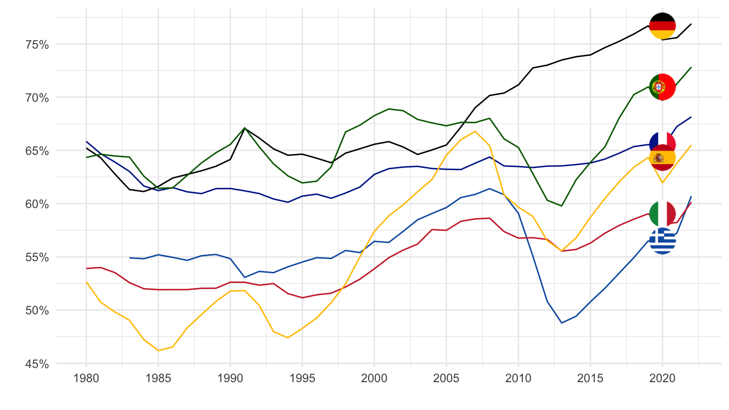
1970-
Code
LFS_SEXAGE_I_R %>%
  filter(SERIES == "EPR",
         AGE == "1564",
         SEX == "MW",
         COUNTRY %in% c("ITA", "DEU", "GRC", "ESP", "PRT", "FRA")) %>%
  year_to_date %>%
  filter(date >= as.Date("1970-01-01")) %>%
  left_join(LFS_SEXAGE_I_R_var$COUNTRY, by = "COUNTRY") %>%
  select(Country, date, obsValue) %>%
  arrange(Country, date) %>%
  ggplot(.) + geom_line(aes(x = date, y = obsValue/100, color = Country)) +
  scale_color_manual(values = c("#002395", "#000000", "#0D5EAF",
                                "#CE2B37", "#006600", "#FFC400")) +
  theme_minimal() + xlab("") + ylab("") +
  geom_image(data = . %>%
               filter(date == as.Date("2019-01-01")) %>%
               mutate(date = as.Date("2020-01-01"),
                      image = paste0("../../icon/flag/round/", str_to_lower(Country), ".png")),
             aes(x = date, y = obsValue/100, image = image), asp = 1.5) +
  scale_x_date(breaks = seq(1960, 2100, 5) %>% paste0("-01-01") %>% as.Date,
               labels = date_format("%Y")) +
  theme(legend.position = "none") +
  scale_y_continuous(breaks = 0.01*seq(0, 200, 5),
                     labels = scales::percent_format(accuracy = 1))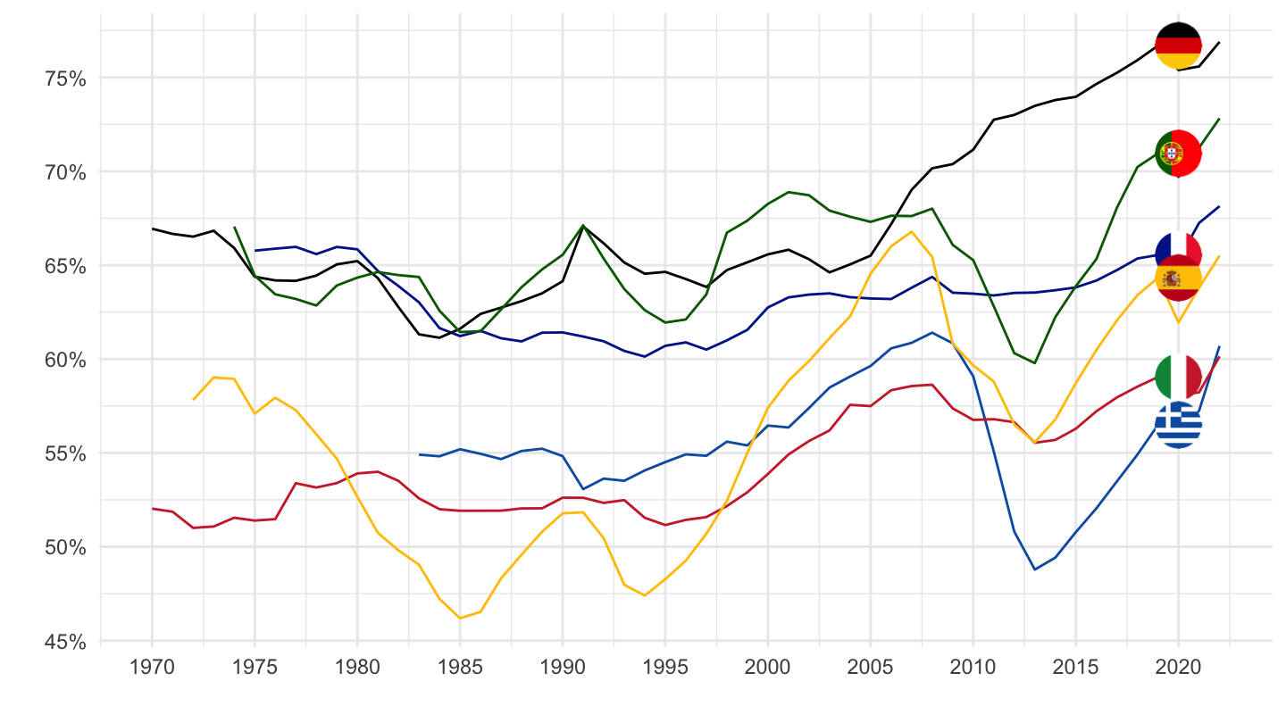
1960-
Code
LFS_SEXAGE_I_R %>%
  filter(SERIES == "EPR",
         AGE == "1564",
         SEX == "MW",
         COUNTRY %in% c("ITA", "DEU", "GRC", "ESP", "PRT", "FRA")) %>%
  year_to_date %>%
  filter(date >= as.Date("1960-01-01")) %>%
  left_join(LFS_SEXAGE_I_R_var$COUNTRY, by = "COUNTRY") %>%
  select(Country, date, obsValue) %>%
  arrange(Country, date) %>%
  ggplot(.) + geom_line(aes(x = date, y = obsValue/100, color = Country)) +
  scale_color_manual(values = c("#002395", "#000000", "#0D5EAF",
                                "#CE2B37", "#006600", "#FFC400")) +
  theme_minimal() + xlab("") + ylab("") +
  geom_image(data = . %>%
               filter(date == as.Date("2019-01-01")) %>%
               mutate(date = as.Date("2021-01-01"),
                      image = paste0("../../icon/flag/round/", str_to_lower(Country), ".png")),
             aes(x = date, y = obsValue/100, image = image), asp = 1.5) +
  scale_x_date(breaks = seq(1960, 2100, 5) %>% paste0("-01-01") %>% as.Date,
               labels = date_format("%Y")) +
  theme(legend.position = "none") +
  scale_y_continuous(breaks = 0.01*seq(0, 200, 5),
                     labels = scales::percent_format(accuracy = 1))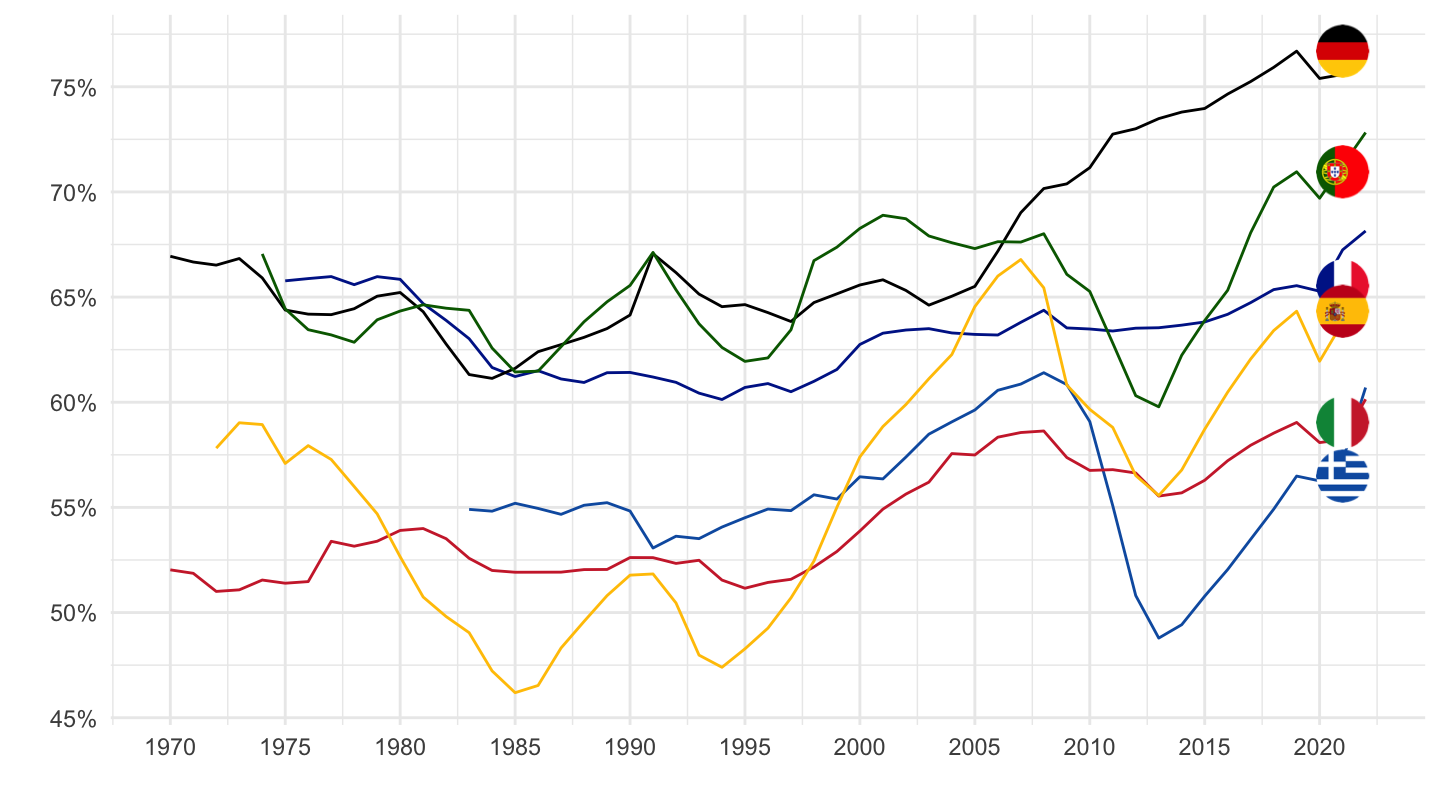
FLAGS & legends
2000-
Code
LFS_SEXAGE_I_R %>%
  filter(SERIES == "EPR",
         AGE == "1564",
         SEX == "MW",
         COUNTRY %in% c("ITA", "DEU", "GRC", "ESP", "PRT", "FRA")) %>%
  year_to_date %>%
  filter(date >= as.Date("2000-01-01")) %>%
  left_join(LFS_SEXAGE_I_R_var$COUNTRY, by = "COUNTRY") %>%
  select(Country, date, obsValue) %>%
  arrange(Country, date) %>%
  ggplot(.) + geom_line(aes(x = date, y = obsValue/100, color = Country)) +
  scale_color_manual(values = c("#002395", "#000000", "#0D5EAF",
                                "#CE2B37", "#006600", "#FFC400")) +
  theme_minimal() + xlab("") + ylab("") +
  geom_image(data = . %>%
               filter(date == as.Date("2019-01-01")) %>%
               mutate(date = as.Date("2020-01-01"),
                      image = paste0("../../icon/flag/round/", str_to_lower(Country), ".png")),
             aes(x = date, y = obsValue/100, image = image), asp = 1.5) +
  scale_x_date(breaks = seq(1960, 2100, 1) %>% paste0("-01-01") %>% as.Date,
               labels = date_format("%Y")) +
  theme(legend.position = c(0.25, 0.9),
        legend.title = element_blank(),
        legend.direction = "horizontal") +
  scale_y_continuous(breaks = 0.01*seq(0, 200, 5),
                     labels = scales::percent_format(accuracy = 1))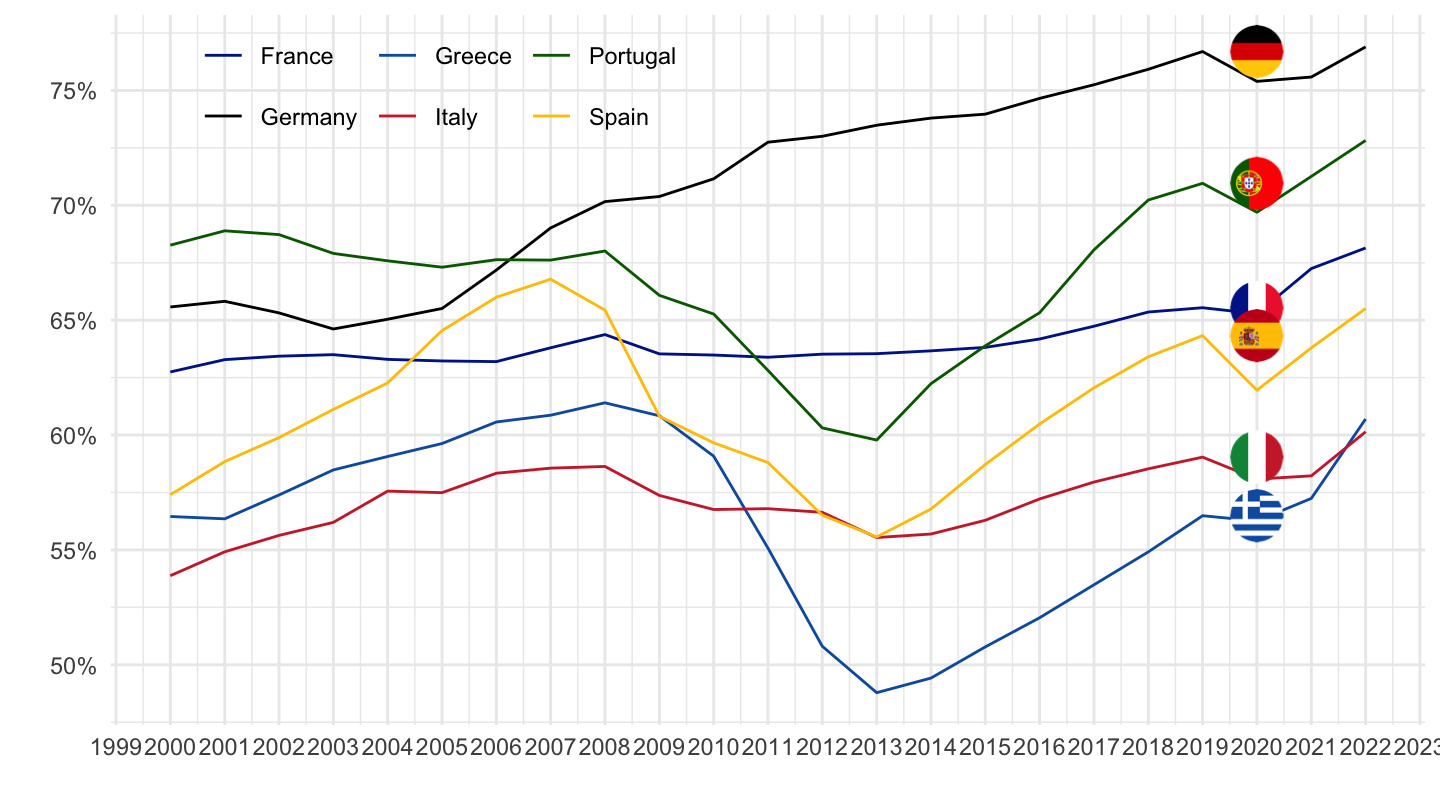
1990-
Code
LFS_SEXAGE_I_R %>%
  filter(SERIES == "EPR",
         AGE == "1564",
         SEX == "MW",
         COUNTRY %in% c("ITA", "DEU", "GRC", "ESP", "PRT", "FRA")) %>%
  year_to_date %>%
  filter(date >= as.Date("1990-01-01")) %>%
  left_join(LFS_SEXAGE_I_R_var$COUNTRY, by = "COUNTRY") %>%
  select(Country, date, obsValue) %>%
  arrange(Country, date) %>%
  ggplot(.) + geom_line(aes(x = date, y = obsValue/100, color = Country)) +
  scale_color_manual(values = c("#002395", "#000000", "#0D5EAF",
                                "#CE2B37", "#006600", "#FFC400")) +
  theme_minimal() + xlab("") + ylab("") +
  geom_image(data = . %>%
               filter(date == as.Date("2019-01-01")) %>%
               mutate(date = as.Date("2020-01-01"),
                      image = paste0("../../icon/flag/round/", str_to_lower(Country), ".png")),
             aes(x = date, y = obsValue/100, image = image), asp = 1.5) +
  scale_x_date(breaks = seq(1960, 2100, 5) %>% paste0("-01-01") %>% as.Date,
               labels = date_format("%Y")) +
  theme(legend.position = c(0.25, 0.9),
        legend.title = element_blank(),
        legend.direction = "horizontal") +
  scale_y_continuous(breaks = 0.01*seq(0, 200, 5),
                     labels = scales::percent_format(accuracy = 1))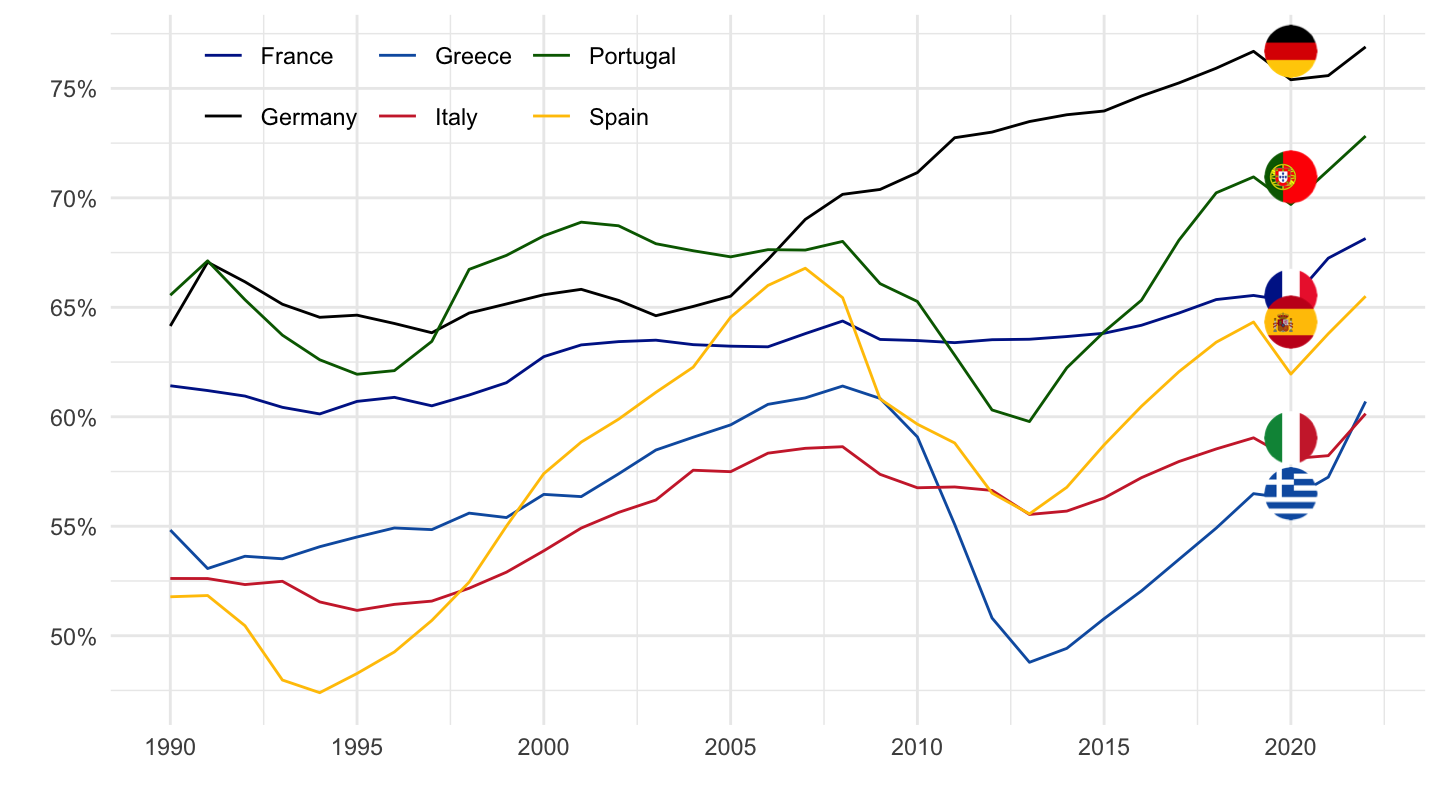
1980-
Code
LFS_SEXAGE_I_R %>%
  filter(SERIES == "EPR",
         AGE == "1564",
         SEX == "MW",
         COUNTRY %in% c("ITA", "DEU", "GRC", "ESP", "PRT", "FRA")) %>%
  year_to_date %>%
  filter(date >= as.Date("1980-01-01")) %>%
  left_join(LFS_SEXAGE_I_R_var$COUNTRY, by = "COUNTRY") %>%
  select(Country, date, obsValue) %>%
  arrange(Country, date) %>%
  ggplot(.) + geom_line(aes(x = date, y = obsValue/100, color = Country)) +
  scale_color_manual(values = c("#002395", "#000000", "#0D5EAF",
                                "#CE2B37", "#006600", "#FFC400")) +
  theme_minimal() + xlab("") + ylab("") +
  geom_image(data = . %>%
               filter(date == as.Date("2019-01-01")) %>%
               mutate(date = as.Date("2020-01-01"),
                      image = paste0("../../icon/flag/round/", str_to_lower(Country), ".png")),
             aes(x = date, y = obsValue/100, image = image), asp = 1.5) +
  scale_x_date(breaks = seq(1960, 2100, 5) %>% paste0("-01-01") %>% as.Date,
               labels = date_format("%Y")) +
  theme(legend.position = c(0.25, 0.9),
        legend.title = element_blank(),
        legend.direction = "horizontal") +
  scale_y_continuous(breaks = 0.01*seq(0, 200, 5),
                     labels = scales::percent_format(accuracy = 1))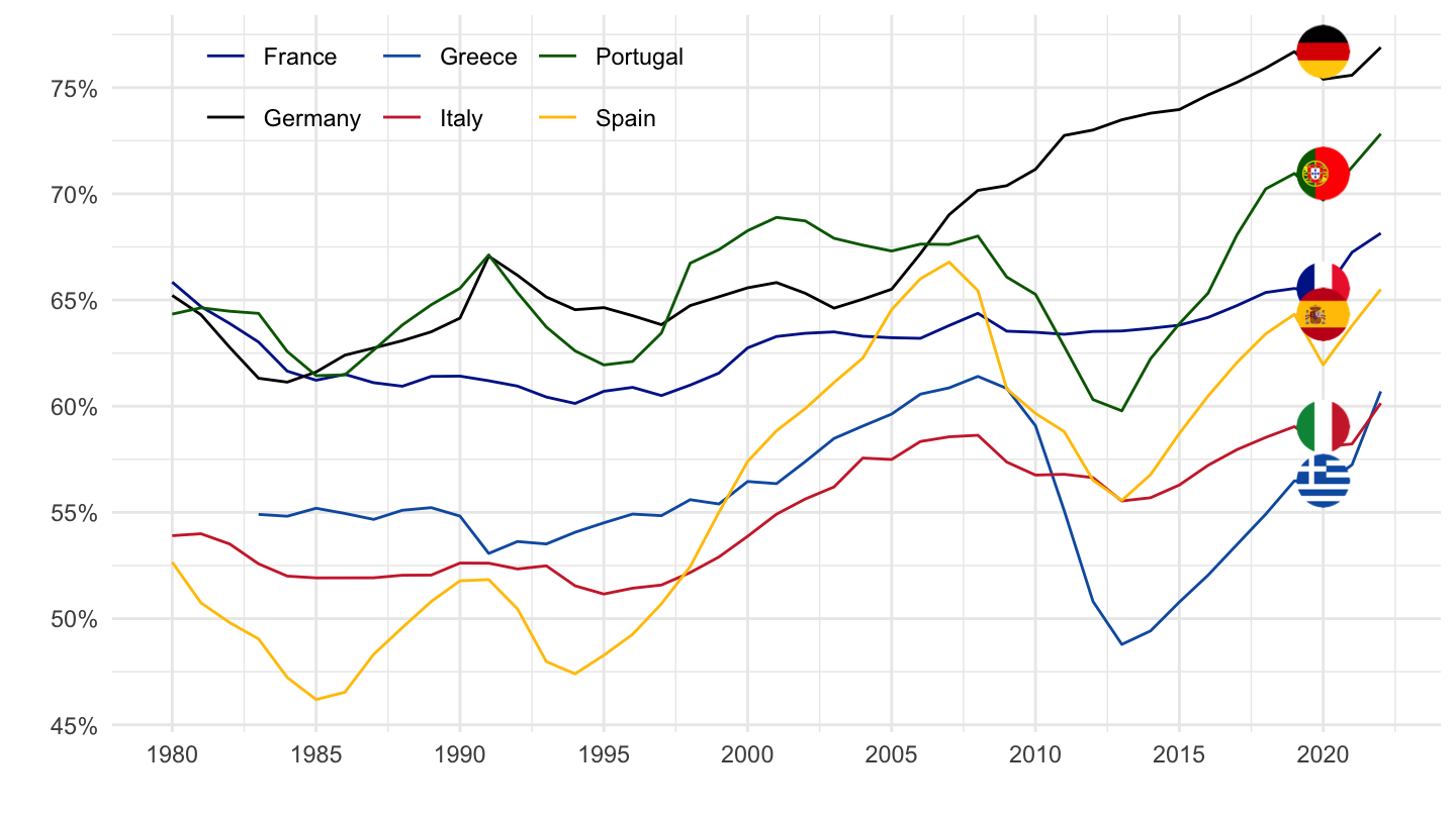
EP - Men
FLAGS
2000-
Code
LFS_SEXAGE_I_R %>%
  filter(SERIES == "EPR",
         AGE == "1564",
         SEX == "MEN",
         COUNTRY %in% c("ITA", "DEU", "GRC", "ESP", "PRT", "FRA")) %>%
  year_to_date %>%
  filter(date >= as.Date("2000-01-01")) %>%
  left_join(LFS_SEXAGE_I_R_var$COUNTRY, by = "COUNTRY") %>%
  select(Country, date, obsValue) %>%
  arrange(Country, date) %>%
  ggplot(.) + geom_line(aes(x = date, y = obsValue/100, color = Country)) +
  scale_color_manual(values = c("#002395", "#000000", "#0D5EAF",
                                "#CE2B37", "#006600", "#FFC400")) +
  theme_minimal() + xlab("") + ylab("Employment / Population (Men, 15-64)") +
  geom_image(data = . %>%
               filter(date == as.Date("2019-01-01")) %>%
               mutate(date = as.Date("2020-01-01"),
                      image = paste0("../../icon/flag/round/", str_to_lower(Country), ".png")),
             aes(x = date, y = obsValue/100, image = image), asp = 1.5) +
  scale_x_date(breaks = seq(1960, 2100, 1) %>% paste0("-01-01") %>% as.Date,
               labels = date_format("%Y")) +
  theme(legend.position = "none") +
  scale_y_continuous(breaks = 0.01*seq(0, 200, 5),
                     labels = scales::percent_format(accuracy = 1))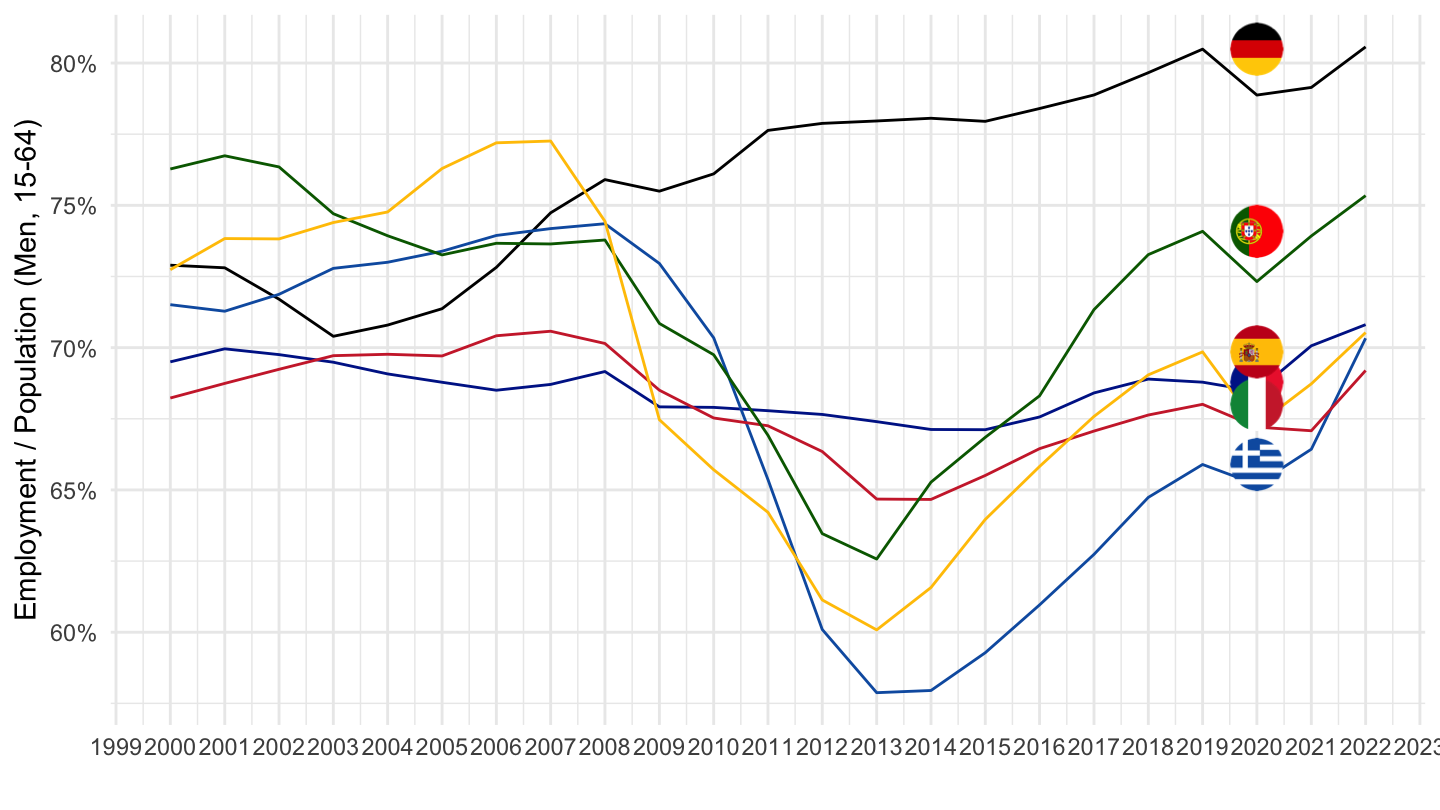
1990-
Code
LFS_SEXAGE_I_R %>%
  filter(SERIES == "EPR",
         AGE == "1564",
         SEX == "MEN",
         COUNTRY %in% c("ITA", "DEU", "GRC", "ESP", "PRT", "FRA")) %>%
  year_to_date %>%
  filter(date >= as.Date("1990-01-01")) %>%
  left_join(LFS_SEXAGE_I_R_var$COUNTRY, by = "COUNTRY") %>%
  select(Country, date, obsValue) %>%
  arrange(Country, date) %>%
  ggplot(.) + geom_line(aes(x = date, y = obsValue/100, color = Country)) +
  scale_color_manual(values = c("#002395", "#000000", "#0D5EAF",
                                "#CE2B37", "#006600", "#FFC400")) +
  theme_minimal() + xlab("") + ylab("Employment / Population (Men, 15-64)") +
  geom_image(data = . %>%
               filter(date == as.Date("2019-01-01")) %>%
               mutate(date = as.Date("2020-01-01"),
                      image = paste0("../../icon/flag/round/", str_to_lower(Country), ".png")),
             aes(x = date, y = obsValue/100, image = image), asp = 1.5) +
  scale_x_date(breaks = seq(1960, 2100, 5) %>% paste0("-01-01") %>% as.Date,
               labels = date_format("%Y")) +
  theme(legend.position = "none") +
  scale_y_continuous(breaks = 0.01*seq(0, 200, 5),
                     labels = scales::percent_format(accuracy = 1))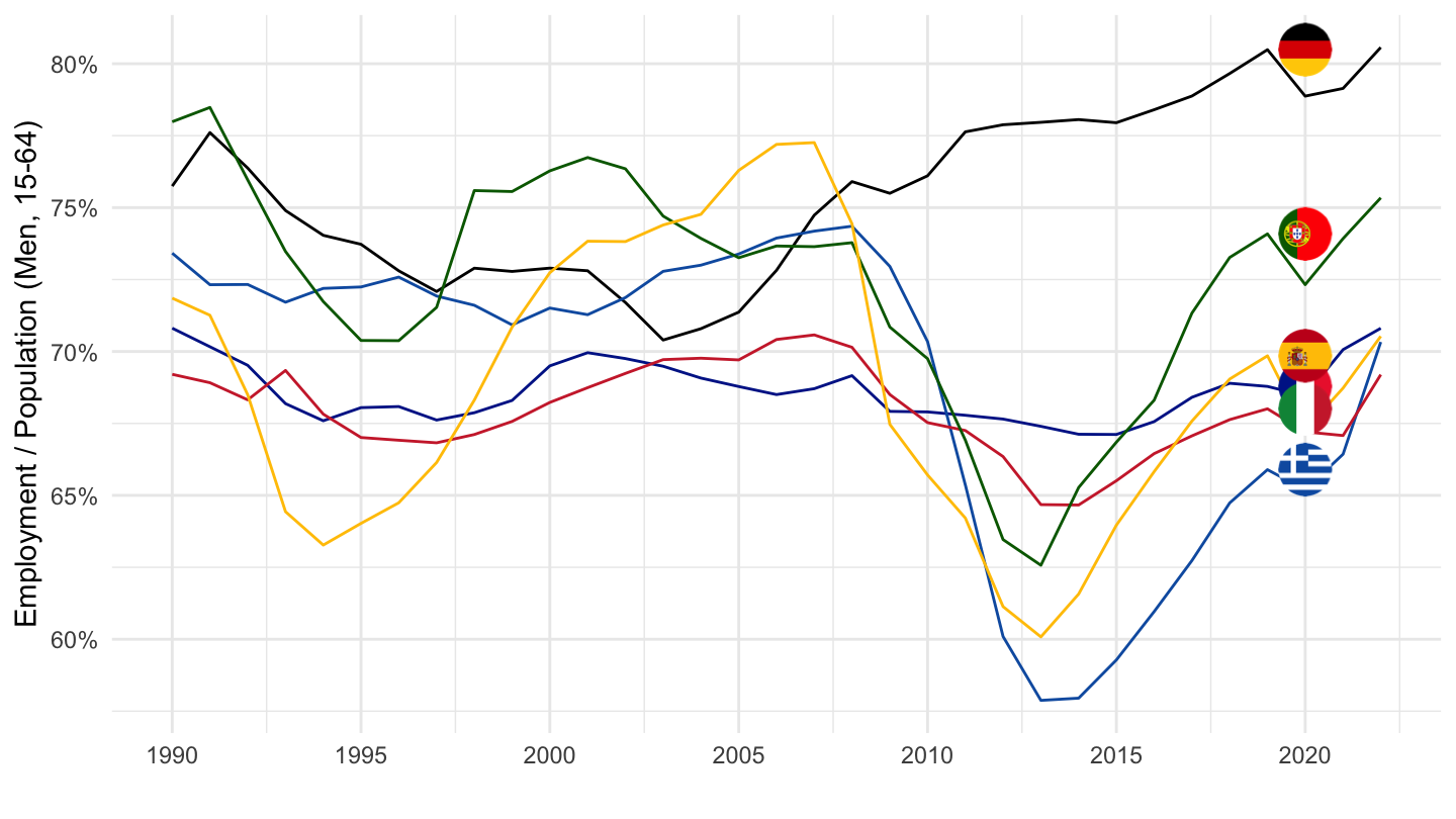
1980-
Code
LFS_SEXAGE_I_R %>%
  filter(SERIES == "EPR",
         AGE == "1564",
         SEX == "MEN",
         COUNTRY %in% c("ITA", "DEU", "GRC", "ESP", "PRT", "FRA")) %>%
  year_to_date %>%
  filter(date >= as.Date("1980-01-01")) %>%
  left_join(LFS_SEXAGE_I_R_var$COUNTRY, by = "COUNTRY") %>%
  select(Country, date, obsValue) %>%
  arrange(Country, date) %>%
  ggplot(.) + geom_line(aes(x = date, y = obsValue/100, color = Country)) +
  scale_color_manual(values = c("#002395", "#000000", "#0D5EAF",
                                "#CE2B37", "#006600", "#FFC400")) +
  theme_minimal() + xlab("") + ylab("") +
  geom_image(data = . %>%
               filter(date == as.Date("2019-01-01")) %>%
               mutate(date = as.Date("2020-01-01"),
                      image = paste0("../../icon/flag/round/", str_to_lower(Country), ".png")),
             aes(x = date, y = obsValue/100, image = image), asp = 1.5) +
  scale_x_date(breaks = seq(1960, 2100, 5) %>% paste0("-01-01") %>% as.Date,
               labels = date_format("%Y")) +
  theme(legend.position = "none") +
  scale_y_continuous(breaks = 0.01*seq(0, 200, 5),
                     labels = scales::percent_format(accuracy = 1))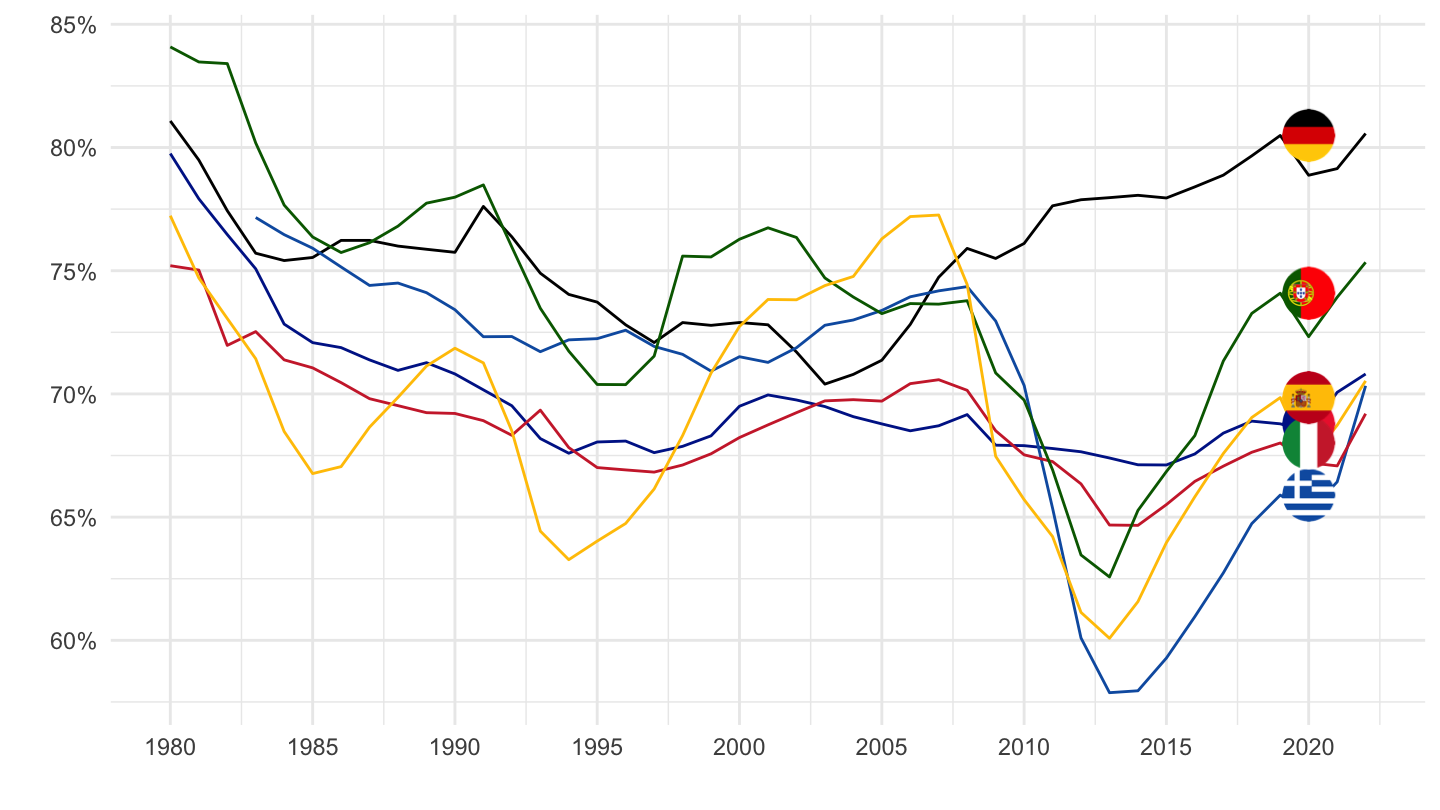
EP - Women
Code
LFS_SEXAGE_I_R %>%
  filter(SERIES == "EPR",
         AGE == "1564",
         SEX == "WOMEN",
         COUNTRY %in% c("ITA", "DEU", "GRC", "ESP", "PRT", "FRA")) %>%
  year_to_date %>%
  filter(date >= as.Date("2000-01-01")) %>%
  left_join(LFS_SEXAGE_I_R_var$COUNTRY, by = "COUNTRY") %>%
  arrange(date) %>%
  ggplot(.) + geom_line(aes(x = date, y = obsValue/100, color = Country, linetype = Country)) +
  scale_color_manual(values = viridis(7)[1:6]) +
  theme_minimal() + xlab("") + ylab("") +
  scale_x_date(breaks = seq(1960, 2100, 1) %>% paste0("-01-01") %>% as.Date,
               labels = date_format("%Y")) +
  theme(legend.position = c(0.25, 0.2),
        legend.title = element_blank(),
        legend.direction = "horizontal") +
  scale_y_continuous(breaks = 0.01*seq(0, 200, 5),
                     labels = scales::percent_format(accuracy = 1))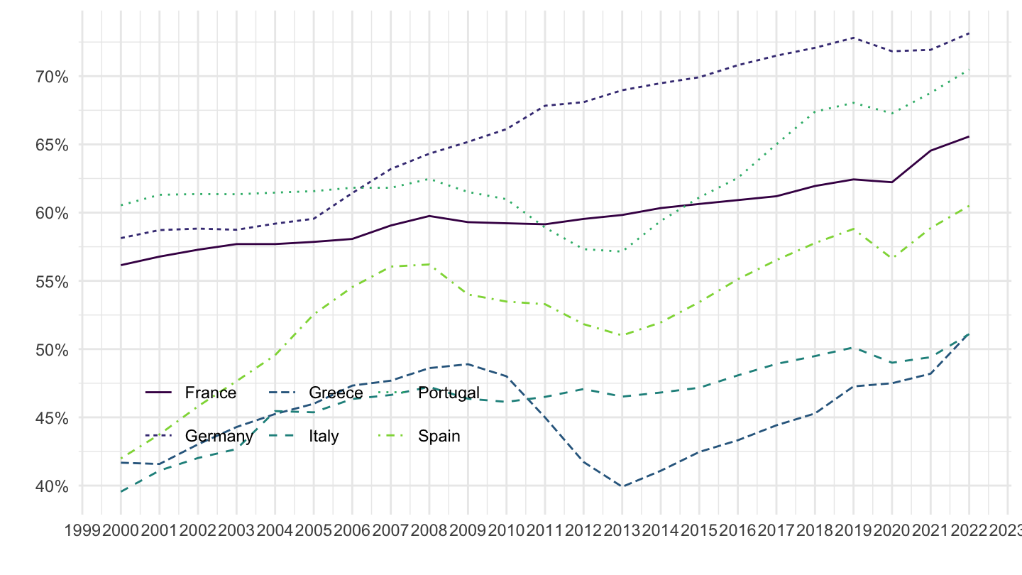
France and Germany
LFP 25-54
Code
LFS_SEXAGE_I_R %>%
  filter(AGE == "2554",
         SEX == "MW",
         COUNTRY %in% c("DEU", "FRA"),
         SERIES == "LFPR") %>%
  left_join(LFS_SEXAGE_I_R_var$COUNTRY, by = "COUNTRY") %>%
  year_to_date %>%
  mutate(obsValue = obsValue/100) %>%
  filter(date >= as.Date("1995-01-01")) %>%
  ggplot() + geom_line(aes(x = date, y = obsValue, color = Country)) +
  scale_color_manual(values = c("#ED2939", "#000000")) +
  theme_minimal() +
  scale_x_date(breaks = seq(1920,   2100, 2) %>% paste0("-01-01") %>% as.Date,
               labels = date_format("%Y")) +
  theme(legend.position = c(0.25, 0.9),
        legend.title = element_blank()) +
  scale_y_continuous(breaks = 0.01*seq(-7, 90, 1),
                     labels = percent_format(accuracy = 1)) +
  ylab("Labor Force Participation Rate (25-54)") + xlab("")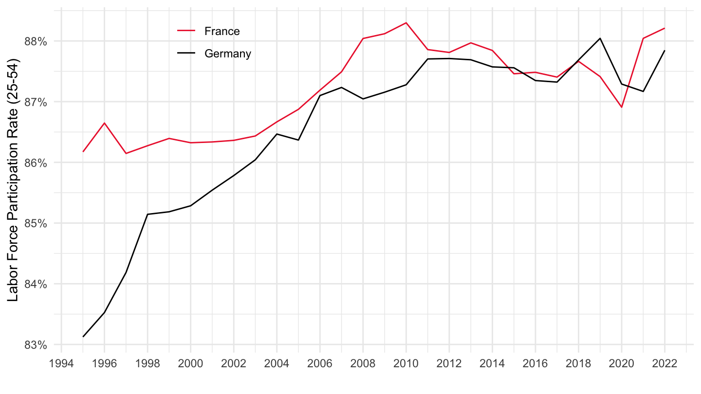
LFP 15-64
Code
LFS_SEXAGE_I_R %>%
  filter(AGE == "1564",
         SEX == "MW",
         COUNTRY %in% c("DEU", "FRA"),
         SERIES == "LFPR") %>%
  left_join(LFS_SEXAGE_I_R_var$COUNTRY, by = "COUNTRY") %>%
  year_to_date %>%
  mutate(obsValue = obsValue/100) %>%
  filter(date >= as.Date("1995-01-01")) %>%
  ggplot() + geom_line(aes(x = date, y = obsValue, color = Country)) +
     scale_color_manual(values = c("#ED2939", "#000000")) +
  theme_minimal() +
  scale_x_date(breaks = seq(1920,   2100, 2) %>% paste0("-01-01") %>% as.Date,
               labels = date_format("%Y")) +
  theme(legend.position = c(0.25, 0.9),
        legend.title = element_blank()) +
  scale_y_continuous(breaks = 0.01*seq(-7, 90, 1),
                     labels = percent_format(accuracy = 1)) +
  ylab("Labor Force Participation Rate (15-64)") + xlab("")
LFP 65+
Code
LFS_SEXAGE_I_R %>%
  filter(AGE == "6599",
         SEX == "MW",
         COUNTRY %in% c("DEU", "FRA"),
         SERIES == "LFPR") %>%
  left_join(LFS_SEXAGE_I_R_var$COUNTRY, by = "COUNTRY") %>%
  year_to_date %>%
  mutate(obsValue = obsValue/100) %>%
  filter(date >= as.Date("1995-01-01")) %>%
  ggplot() + geom_line(aes(x = date, y = obsValue, color = Country, linetype = Country)) +
     scale_color_manual(values = c("#ED2939", "#000000")) +
  theme_minimal() +
  scale_x_date(breaks = seq(1920,   2100, 2) %>% paste0("-01-01") %>% as.Date,
               labels = date_format("%Y")) +
  theme(legend.position = c(0.25, 0.9),
        legend.title = element_blank()) +
  scale_y_continuous(breaks = 0.01*seq(-7, 90, 1),
                     labels = percent_format(accuracy = 1)) +
  ylab("Labor Force Participation Rate (65+)") + xlab("")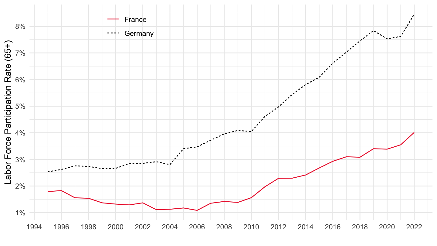
LFP 65-69
Code
LFS_SEXAGE_I_R %>%
  filter(AGE == "6569",
         SEX == "MW",
         COUNTRY %in% c("DEU", "FRA"),
         SERIES == "LFPR") %>%
  left_join(LFS_SEXAGE_I_R_var$COUNTRY, by = "COUNTRY") %>%
  year_to_date %>%
  mutate(obsValue = obsValue/100) %>%
  filter(date >= as.Date("1995-01-01")) %>%
  ggplot() + geom_line(aes(x = date, y = obsValue, color = Country, linetype = Country)) +
     scale_color_manual(values = c("#ED2939", "#000000")) +
  theme_minimal() +
  scale_x_date(breaks = seq(1920,   2100, 2) %>% paste0("-01-01") %>% as.Date,
               labels = date_format("%Y")) +
  theme(legend.position = c(0.25, 0.9),
        legend.title = element_blank()) +
  scale_y_continuous(breaks = 0.01*seq(-7, 90, 1),
                     labels = percent_format(accuracy = 1)) +
  ylab("Labor Force Participation Rate (65-69)") + xlab("")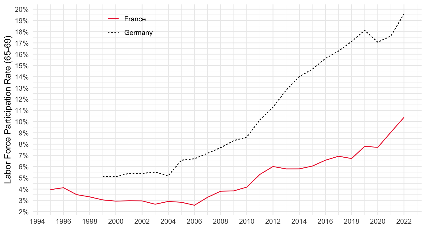
EP 65-69
Code
LFS_SEXAGE_I_R %>%
  filter(AGE == "6569",
         SEX == "MW",
         COUNTRY %in% c("DEU", "FRA"),
         SERIES == "EPR") %>%
  left_join(LFS_SEXAGE_I_R_var$COUNTRY, by = "COUNTRY") %>%
  year_to_date %>%
  mutate(obsValue = obsValue/100) %>%
  filter(date >= as.Date("1995-01-01")) %>%
  ggplot() + geom_line(aes(x = date, y = obsValue, color = Country, linetype = Country)) +
     scale_color_manual(values = c("#ED2939", "#000000")) +
  theme_minimal() +
  scale_x_date(breaks = seq(1920,   2100, 2) %>% paste0("-01-01") %>% as.Date,
               labels = date_format("%Y")) +
  theme(legend.position = c(0.25, 0.9),
        legend.title = element_blank()) +
  scale_y_continuous(breaks = 0.01*seq(-7, 90, 1),
                     labels = percent_format(accuracy = 1)) +
  ylab("Employment/Population Ratio (65-69)") + xlab("")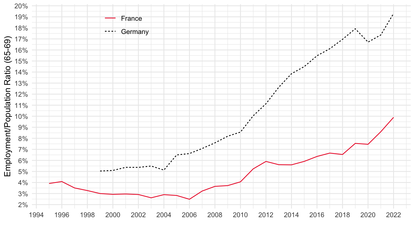
EP 25-54
Code
LFS_SEXAGE_I_R %>%
  filter(AGE == "2554",
         SEX == "MW",
         COUNTRY %in% c("DEU", "FRA"),
         SERIES == "EPR") %>%
  left_join(LFS_SEXAGE_I_R_var$COUNTRY, by = "COUNTRY") %>%
  year_to_date %>%
  mutate(obsValue = obsValue/100) %>%
  filter(date >= as.Date("1995-01-01")) %>%
  ggplot() + geom_line(aes(x = date, y = obsValue, color = Country)) +
     scale_color_manual(values = c("#ED2939", "#000000")) +
  theme_minimal() +
  scale_x_date(breaks = seq(1920,   2100, 2) %>% paste0("-01-01") %>% as.Date,
               labels = date_format("%Y")) +
  theme(legend.position = c(0.25, 0.9),
        legend.title = element_blank()) +
  scale_y_continuous(breaks = 0.01*seq(-7, 90, 1),
                     labels = percent_format(accuracy = 1)) +
  ylab("Employment / Population Ratio (25-54)") + xlab("")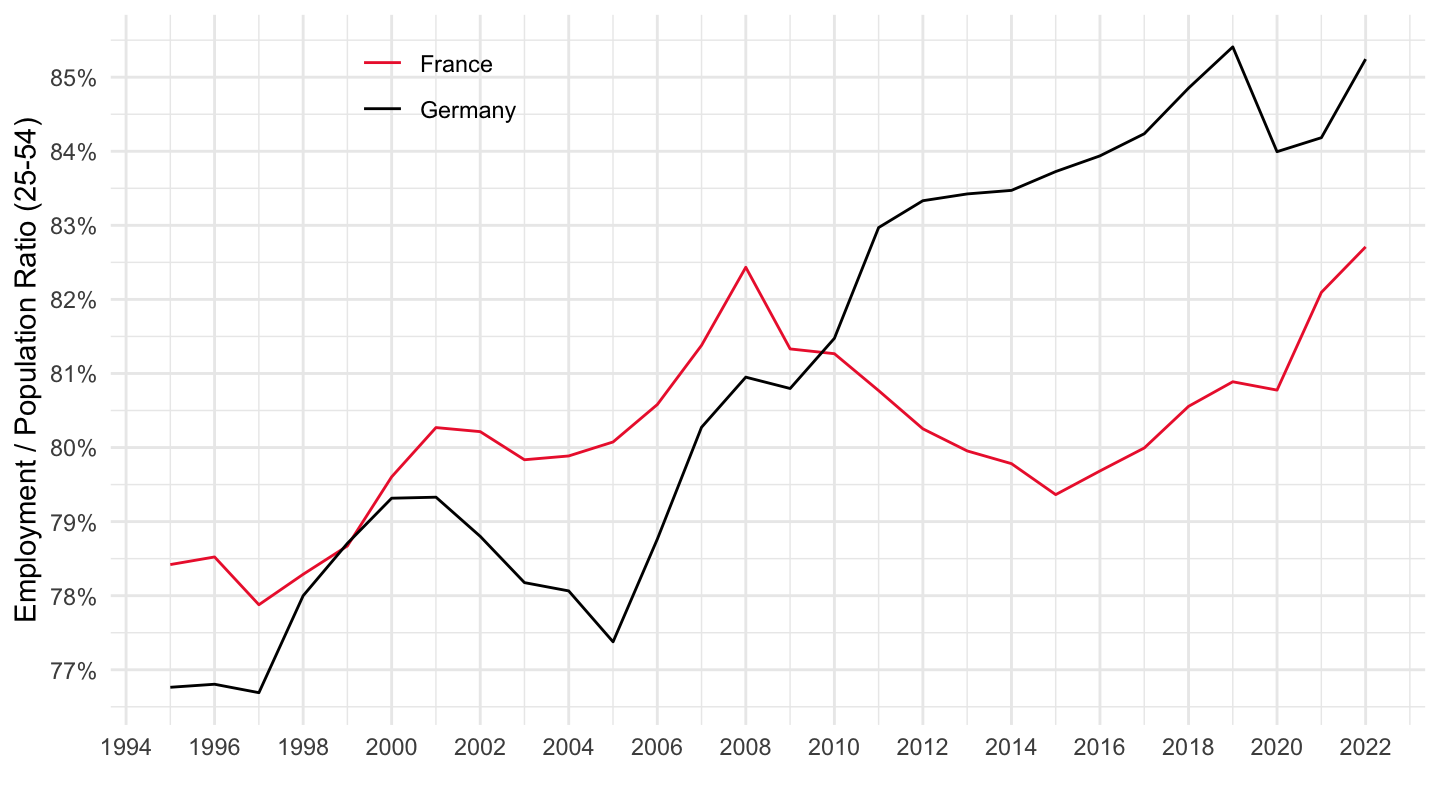
LFP, 25-54, Women
Code
LFS_SEXAGE_I_R %>%
  filter(AGE == "2554",
         SEX == "WOMEN",
         COUNTRY %in% c("DEU", "FRA"),
         SERIES == "LFPR") %>%
  left_join(LFS_SEXAGE_I_R_var$COUNTRY, by = "COUNTRY") %>%
  year_to_date %>%
  mutate(obsValue = obsValue/100) %>%
  filter(date >= as.Date("1995-01-01")) %>%
  ggplot() + geom_line(aes(x = date, y = obsValue, color = Country)) +
     scale_color_manual(values = c("#ED2939", "#000000")) +
  theme_minimal() +
  scale_x_date(breaks = seq(1920,   2100, 2) %>% paste0("-01-01") %>% as.Date,
               labels = date_format("%Y")) +
  theme(legend.position = c(0.25, 0.9),
        legend.title = element_blank()) +
  scale_y_continuous(breaks = 0.01*seq(-7, 90, 1),
                     labels = percent_format(accuracy = 1)) +
  ylab("Labor Force Participation Rate (25-54)") + xlab("")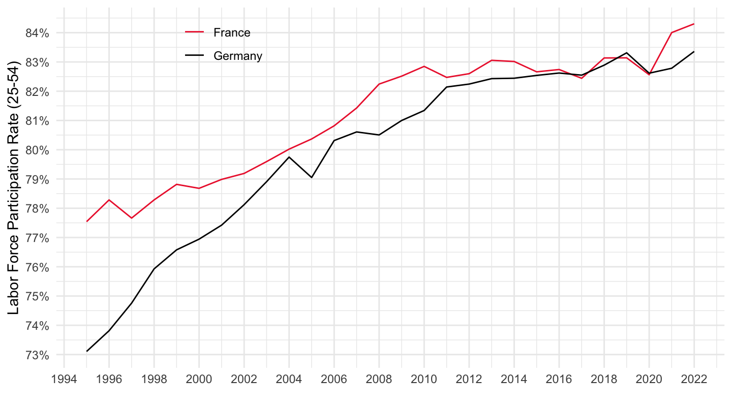
Germany (Men, Women, All)
Code
LFS_SEXAGE_I_R %>%
  filter(AGE == "2554",
         SEX %in% c("MW", "MEN", "WOMEN"),
         COUNTRY %in% c("DEU"),
         SERIES == "EPR") %>%
  left_join(LFS_SEXAGE_I_R_var$SEX, by = "SEX") %>%
  year_to_date %>%
  mutate(obsValue = obsValue/100) %>%
  ggplot() + geom_line(aes(x = date, y = obsValue, color = Sex)) +
  theme_minimal() +
  scale_x_date(breaks = seq(1920,   2100, 2) %>% paste0("-01-01") %>% as.Date,
               labels = date_format("%Y")) +
  theme(legend.position = c(0.75, 0.2),
        legend.title = element_blank()) +
  scale_y_continuous(breaks = 0.01*seq(10, 100, 5),
                     labels = percent_format(accuracy = 1)) +
  ylab("Employment / Population Ratio (25-54)") + xlab("")