Short-Term Labour Market Statistics
Data - OECD
Info
Data on employment
| source | dataset | Title | .html | .rData |
|---|---|---|---|---|
| oecd | STLABOUR | Short-Term Labour Market Statistics | 2026-07-23 | 2025-01-17 |
| bls | jt | NA | NA | NA |
| bls | la | NA | NA | NA |
| bls | ln | NA | NA | NA |
| eurostat | nama_10_a10_e | Employment by A*10 industry breakdowns | 2026-07-23 | 2026-07-23 |
| eurostat | nama_10_a64_e | National accounts employment data by industry (up to NACE A*64) | 2026-07-23 | 2026-07-23 |
| eurostat | namq_10_a10_e | Employment A*10 industry breakdowns | 2026-07-23 | 2026-07-23 |
| eurostat | une_rt_m | Unemployment by sex and age – monthly data | 2026-07-23 | 2026-07-23 |
| oecd | ALFS_EMP | Employment by activities and status (ALFS) | 2024-04-16 | 2025-05-24 |
| oecd | EPL_T | Strictness of employment protection – temporary contracts | 2026-07-23 | 2023-12-10 |
| oecd | LFS_SEXAGE_I_R | LFS by sex and age - indicators | 2026-07-23 | 2024-04-15 |
LAST_COMPILE
| LAST_COMPILE |
|---|
| 2026-07-24 |
Last
| obsTime | Nobs |
|---|---|
| 2020-Q4 | 16660 |
Nobs - Javascript
Code
STLABOUR %>%
  left_join(STLABOUR_var$SUBJECT, by = "SUBJECT") %>%
  left_join(STLABOUR_var$MEASURE, by = "MEASURE") %>%
  group_by(SUBJECT, Subject, MEASURE, Measure, FREQUENCY) %>%
  summarise(Nobs = n()) %>%
  arrange(-Nobs) %>%
  {if (is_html_output()) datatable(., filter = 'top', rownames = F) else .}
SUBJECT
Code
STLABOUR %>%
  left_join(STLABOUR_var$SUBJECT, by = "SUBJECT") %>%
  group_by(SUBJECT, Subject) %>%
  summarise(Nobs = n()) %>%
  arrange(-Nobs) %>%
  {if (is_html_output()) datatable(., filter = 'top', rownames = F) else .}
MEASURE
Code
STLABOUR %>%
  left_join(STLABOUR_var$MEASURE, by = "MEASURE") %>%
  group_by(MEASURE, Measure) %>%
  summarise(Nobs = n()) %>%
  arrange(-Nobs) %>%
{if (is_html_output()) print_table(.) else .}| MEASURE | Measure | Nobs |
|---|---|---|
| ST | Level, rate or quantity series | 1631452 |
| STSA | Level, rate or quantity series, s.a. | 1575508 |
| GPSA | Growth previous period, s.a. | 131395 |
| GP | Growth previous period | 123475 |
| EMP | NA | 38715 |
| LF | NA | 20230 |
| UNE | NA | 17046 |
| EMP_WAP | NA | 17044 |
| OLF | NA | 16865 |
| WAP | NA | 16805 |
| UNE_LF | NA | 16567 |
| OLF_WAP | NA | 16485 |
| LF_WAP | NA | 16393 |
| UNE_LF_M | NA | 11700 |
| UNE_M | NA | 7800 |
| EES | NA | 966 |
| UNE_LT | NA | 20 |
| UNE_ST | NA | 20 |
FREQUENCY
Code
STLABOUR %>%
  left_join(STLABOUR_var$FREQUENCY, by = "FREQUENCY") %>%
  group_by(FREQUENCY, Frequency) %>%
  summarise(Nobs = n()) %>%
  arrange(-Nobs) %>%
{if (is_html_output()) print_table(.) else .}| FREQUENCY | Frequency | Nobs |
|---|---|---|
| Q | Quarterly | 1610307 |
| M | Monthly | 1430909 |
| A | Annual | 420614 |
| NA | NA | 196656 |
LOCATION
Code
STLABOUR %>%
  left_join(STLABOUR_var$LOCATION, by = "LOCATION") %>%
  group_by(LOCATION, Location) %>%
  summarise(Nobs = n()) %>%
  arrange(-Nobs) %>%
  mutate(Flag = gsub(" ", "-", str_to_lower(Location)),
         Flag = paste0('<img src="../../icon/flag/vsmall/', Flag, '.png" alt="Flag">')) %>%
  select(Flag, everything()) %>%
  {if (is_html_output()) datatable(., filter = 'top', rownames = F, escape = F) else .}
Employment to Population Rate - LREPTTMA
Table
Code
STLABOUR %>%
  # LREMTTTT: Harmonised unemployment Rate (monthly), Total, All persons
  # ST: Level, rate or quantity series
  filter(SUBJECT %in% c("LREPTTTT"),
         MEASURE == "ST") %>%
  left_join(STLABOUR_var$LOCATION, by = "LOCATION") %>%
  left_join(STLABOUR_var$FREQUENCY, by = "FREQUENCY") %>%
  group_by(LOCATION, Location, Frequency) %>%
  summarise(Nobs = n()) %>%
  spread(Frequency, Nobs) %>%
  arrange(-`Annual`) %>%
  mutate(Flag = gsub(" ", "-", str_to_lower(Location)),
         Flag = paste0('<img src="../../icon/flag/vsmall/', Flag, '.png" alt="Flag">')) %>%
  select(Flag, everything()) %>%
  {if (is_html_output()) datatable(., filter = 'top', rownames = F, escape = F) else .}
Employment rate
Table
Code
STLABOUR %>%
  # LREMTTTT: Harmonised unemployment Rate (monthly), Total, All persons
  # ST: Level, rate or quantity series
  filter(SUBJECT %in% c("LREMTTTT", "LREM25TT", "LREM64TT", "LREM74TT"),
         MEASURE == "ST",
         FREQUENCY == "A") %>%
  left_join(STLABOUR_var$LOCATION, by = "LOCATION") %>%
  left_join(STLABOUR_var$SUBJECT, by = "SUBJECT") %>%
  group_by(LOCATION, Location, Subject) %>%
  summarise(Nobs = n()) %>%
  spread(Subject, Nobs) %>%
  arrange(-`Employment rate, Aged 15 and over, All persons`) %>%
  mutate(Flag = gsub(" ", "-", str_to_lower(Location)),
         Flag = paste0('<img src="../../icon/flag/vsmall/', Flag, '.png" alt="Flag">')) %>%
  select(Flag, everything()) %>%
  {if (is_html_output()) datatable(., filter = 'top', rownames = F, escape = F) else .}
Italy, Germany, France, Spain, Greece
25-54
Code
STLABOUR %>%
  filter(SUBJECT %in% c("LREM25TT"),
         MEASURE == "ST",
         FREQUENCY == "Q",
         LOCATION %in% c("DEU", "ESP", "FRA", "ITA", "USA")) %>%
  quarter_to_date %>%
  group_by(date) %>%
  filter(n() > 1) %>%
  left_join(STLABOUR_var$LOCATION, by = "LOCATION") %>%
  left_join(colors, by = c("Location" = "country")) %>%
  mutate(obsValue = obsValue/100) %>%
  mutate(color = ifelse(LOCATION == "USA", color2, color)) %>%
  ggplot(.) + geom_line(aes(x = date, y = obsValue, color = color)) +
  scale_color_identity() + add_5flags +
  theme_minimal() + xlab("") + ylab("Employment rate, Aged 25-54") +
  scale_x_date(breaks = seq(1960, 2100, 2) %>% paste0("-01-01") %>% as.Date,
               labels = date_format("%Y")) +
  theme(legend.position = "none") +
  scale_y_continuous(breaks = 0.01*seq(0, 200, 5),
                     labels = scales::percent_format(accuracy = 1))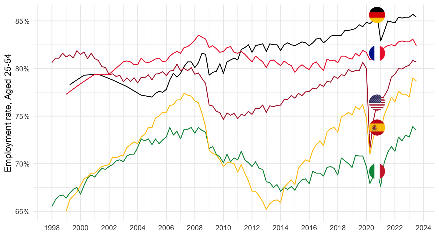
25-64
Code
STLABOUR %>%
  filter(SUBJECT %in% c("LREM64TT"),
         MEASURE == "ST",
         FREQUENCY == "Q",
         LOCATION %in% c("DEU", "ESP", "FRA", "ITA", "USA")) %>%
  quarter_to_date %>%
  group_by(date) %>%
  filter(n() > 1) %>%
  left_join(STLABOUR_var$LOCATION, by = "LOCATION") %>%
  left_join(colors, by = c("Location" = "country")) %>%
  mutate(obsValue = obsValue/100) %>%
  mutate(color = ifelse(LOCATION == "USA", color2, color)) %>%
  ggplot(.) + geom_line(aes(x = date, y = obsValue, color = color)) +
  scale_color_identity() + add_5flags +
  theme_minimal() + xlab("") + ylab("Employment rate, Aged 15-64") +
  scale_x_date(breaks = seq(1960, 2100, 2) %>% paste0("-01-01") %>% as.Date,
               labels = date_format("%Y")) +
  theme(legend.position = "none") +
  scale_y_continuous(breaks = 0.01*seq(0, 200, 5),
                     labels = scales::percent_format(accuracy = 1))
15-74
English
Code
STLABOUR %>%
  filter(SUBJECT %in% c("LREM74TT"),
         MEASURE == "ST",
         FREQUENCY == "Q",
         LOCATION %in% c("DEU", "ESP", "FRA", "ITA", "USA")) %>%
  quarter_to_date %>%
  group_by(date) %>%
  filter(n() > 1) %>%
  left_join(STLABOUR_var$LOCATION, by = "LOCATION") %>%
  left_join(colors, by = c("Location" = "country")) %>%
  mutate(obsValue = obsValue/100) %>%
  mutate(color = ifelse(LOCATION == "USA", color2, color)) %>%
  ggplot(.) + geom_line(aes(x = date, y = obsValue, color = color)) +
  scale_color_identity() + add_5flags +
  theme_minimal() + xlab("") + ylab("Employment rate, Aged 15-74") +
  scale_x_date(breaks = seq(1960, 2100, 2) %>% paste0("-01-01") %>% as.Date,
               labels = date_format("%Y")) +
  theme(legend.position = "none") +
  scale_y_continuous(breaks = 0.01*seq(0, 200, 5),
                     labels = scales::percent_format(accuracy = 1))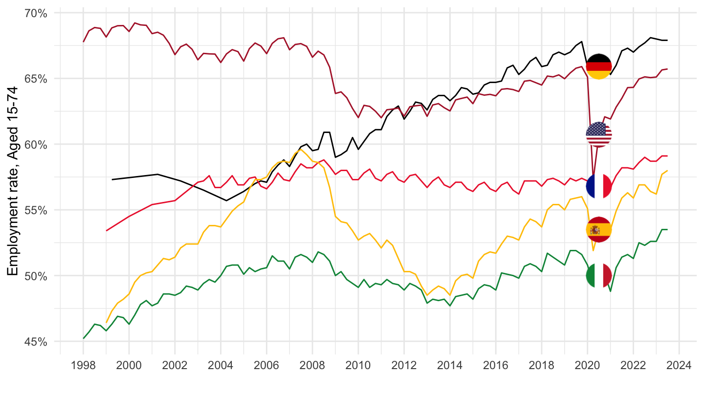
French
Code
STLABOUR %>%
  filter(SUBJECT %in% c("LREM74TT"),
         MEASURE == "ST",
         FREQUENCY == "Q",
         LOCATION %in% c("DEU", "ESP", "FRA", "ITA", "USA")) %>%
  quarter_to_date %>%
  group_by(date) %>%
  filter(n() > 1) %>%
  left_join(STLABOUR_var$LOCATION, by = "LOCATION") %>%
  left_join(colors, by = c("Location" = "country")) %>%
  mutate(obsValue = obsValue/100) %>%
  mutate(color = ifelse(LOCATION == "USA", color2, color)) %>%
  ggplot(.) + geom_line(aes(x = date, y = obsValue, color = color)) +
  scale_color_identity() + add_5flags +
  theme_minimal() + xlab("") + ylab("Taux d'emploi, 15-74") +
  scale_x_date(breaks = seq(1960, 2100, 2) %>% paste0("-01-01") %>% as.Date,
               labels = date_format("%Y")) +
  theme(legend.position = "none") +
  scale_y_continuous(breaks = 0.01*seq(0, 200, 5),
                     labels = scales::percent_format(accuracy = 1))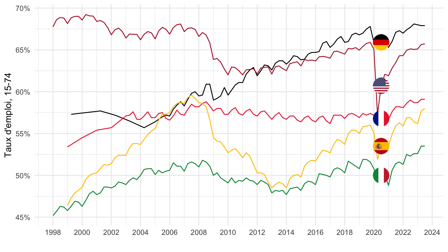
15+
All
Code
STLABOUR %>%
  filter(SUBJECT %in% c("LREMTTTT"),
         MEASURE == "ST",
         FREQUENCY == "Q",
         LOCATION %in% c("DEU", "ESP", "FRA", "ITA", "USA")) %>%
  quarter_to_date %>%
  group_by(date) %>%
  filter(n() > 1) %>%
  left_join(STLABOUR_var$LOCATION, by = "LOCATION") %>%
  left_join(colors, by = c("Location" = "country")) %>%
  mutate(obsValue = obsValue/100) %>%
  mutate(color = ifelse(LOCATION == "USA", color2, color)) %>%
  ggplot(.) + geom_line(aes(x = date, y = obsValue, color = color)) +
  scale_color_identity() + add_5flags +
  theme_minimal() + xlab("") + ylab("Employment rate, Aged 15+") +
  scale_x_date(breaks = seq(1960, 2100, 2) %>% paste0("-01-01") %>% as.Date,
               labels = date_format("%Y")) +
  theme(legend.position = "none") +
  scale_y_continuous(breaks = 0.01*seq(0, 200, 5),
                     labels = scales::percent_format(accuracy = 1))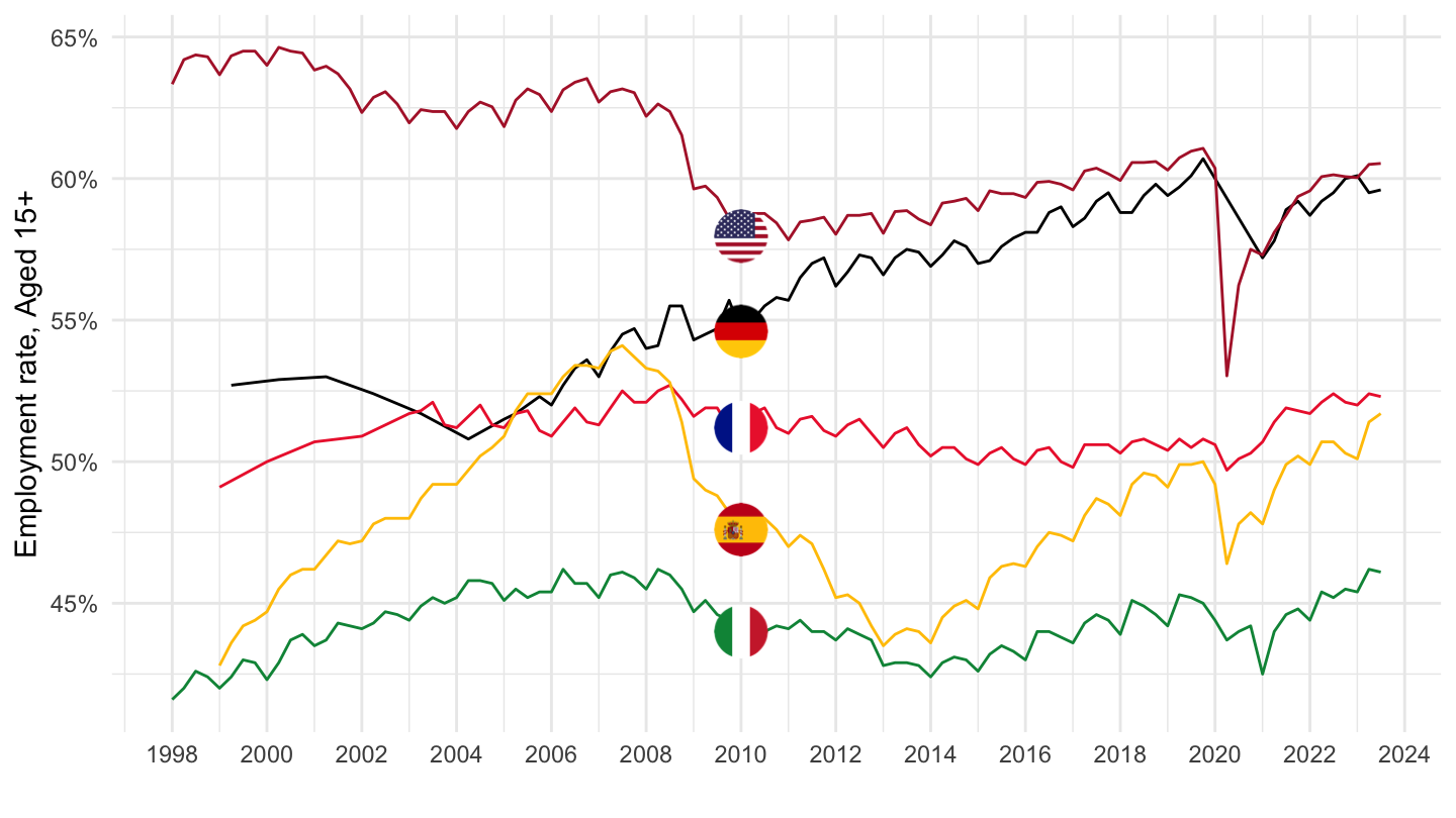
SA
Code
STLABOUR %>%
  filter(SUBJECT %in% c("LREMTTTT"),
         MEASURE == "STSA",
         FREQUENCY == "Q",
         LOCATION %in% c("DEU", "ESP", "FRA", "ITA", "USA")) %>%
  quarter_to_date %>%
  group_by(date) %>%
  filter(n() > 1) %>%
  left_join(STLABOUR_var$LOCATION, by = "LOCATION") %>%
  left_join(colors, by = c("Location" = "country")) %>%
  mutate(obsValue = obsValue/100) %>%
  mutate(color = ifelse(LOCATION == "USA", color2, color)) %>%
  ggplot(.) + geom_line(aes(x = date, y = obsValue, color = color)) +
  scale_color_identity() + add_5flags +
  theme_minimal() + xlab("") + ylab("Employment rate, Aged 15+") +
  scale_x_date(breaks = seq(1960, 2100, 5) %>% paste0("-01-01") %>% as.Date,
               labels = date_format("%Y")) +
  theme(legend.position = "none") +
  scale_y_continuous(breaks = 0.01*seq(0, 200, 5),
                     labels = scales::percent_format(accuracy = 1))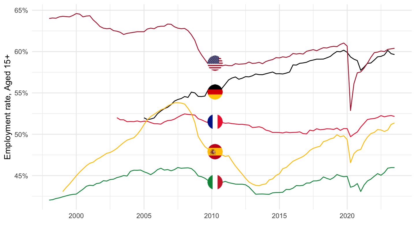
Employment rate - LREMTTTT, LREM25TT, LREM64TT, LREM74TT
Table
Code
STLABOUR %>%
  # LREMTTTT: Harmonised unemployment Rate (monthly), Total, All persons
  # ST: Level, rate or quantity series
  filter(SUBJECT %in% c("LREMTTTT", "LREM25TT", "LREM64TT", "LREM74TT"),
         MEASURE == "ST",
         FREQUENCY == "A") %>%
  left_join(STLABOUR_var$LOCATION, by = "LOCATION") %>%
  left_join(STLABOUR_var$SUBJECT, by = "SUBJECT") %>%
  group_by(LOCATION, Location, Subject) %>%
  summarise(Nobs = n()) %>%
  spread(Subject, Nobs) %>%
  arrange(-`Employment rate, Aged 15 and over, All persons`) %>%
  mutate(Flag = gsub(" ", "-", str_to_lower(Location)),
         Flag = paste0('<img src="../../icon/flag/vsmall/', Flag, '.png" alt="Flag">')) %>%
  select(Flag, everything()) %>%
  {if (is_html_output()) datatable(., filter = 'top', rownames = F, escape = F) else .}
Italy
Absolute
Code
STLABOUR %>%
  # LRHUTTTT: Harmonised unemployment Rate (monthly), Total, All persons
  # ST: Level, rate or quantity series
  filter(SUBJECT %in% c("LREMTTTT", "LREM25TT", "LREM64TT", "LREM74TT"),
         MEASURE == "ST",
         FREQUENCY == "A",
         LOCATION == "ITA") %>%
  left_join(STLABOUR_var$SUBJECT, by = "SUBJECT") %>%
  frequency_to_date %>%
  ggplot() + geom_line() + theme_minimal() +
  aes(x = date, y = obsValue/100, color = Subject) +
  scale_color_manual(values = viridis(5)[1:4]) +
  scale_x_date(breaks = seq(1920, 2100, 5) %>% paste0("-01-01") %>% as.Date,
               labels = date_format("%Y")) +
  theme(legend.position = c(0.6, 0.8),
        legend.title = element_blank()) +
  scale_y_continuous(breaks = 0.01*seq(0, 80, 5),
                     labels = scales::percent_format(accuracy = 1)) +
  ylab("Employment Rate (%)") + xlab("")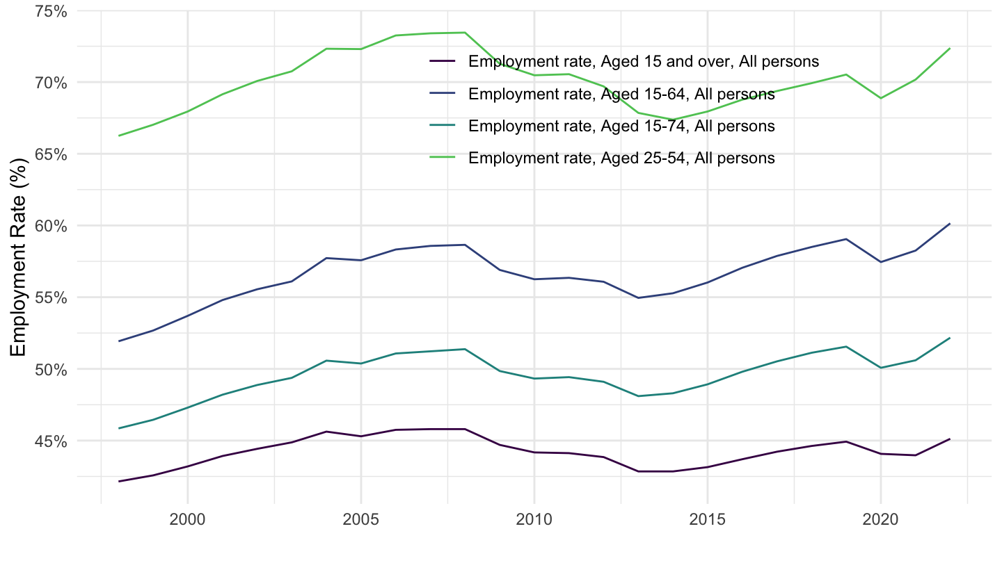
1998 = 100
Code
STLABOUR %>%
  filter(SUBJECT %in% c("LREMTTTT", "LREM25TT", "LREM64TT", "LREM74TT"),
         MEASURE == "ST",
         FREQUENCY == "A",
         LOCATION == "ITA") %>%
  left_join(STLABOUR_var$SUBJECT, by = "SUBJECT") %>%
  frequency_to_date %>%
  group_by(Subject) %>%
  mutate(obsValue = 100*obsValue/obsValue[date == as.Date("1998-01-01")]) %>%
  ggplot() + geom_line() + theme_minimal() +
  aes(x = date, y = obsValue, color = Subject) +
  scale_color_manual(values = viridis(5)[1:4]) +
  scale_x_date(breaks = seq(1920, 2100, 5) %>% paste0("-01-01") %>% as.Date,
               labels = date_format("%Y")) +
  theme(legend.position = c(0.6, 0.8),
        legend.title = element_blank()) +
  scale_y_continuous(breaks = seq(0, 200, 2)) +
  ylab("Employment (1998 = 100)") + xlab("")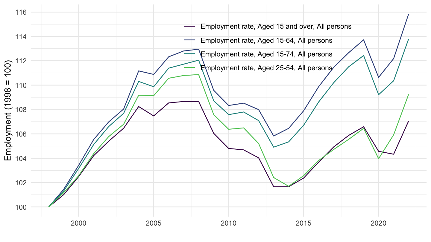
2005 = 100
All
Code
STLABOUR %>%
  filter(SUBJECT %in% c("LREMTTTT", "LREM25TT", "LREM64TT", "LREM74TT"),
         MEASURE == "ST",
         FREQUENCY == "A",
         LOCATION == "ITA") %>%
  left_join(STLABOUR_var$SUBJECT, by = "SUBJECT") %>%
  frequency_to_date %>%
  filter(date >= as.Date("2005-01-01")) %>%
  group_by(Subject) %>%
  mutate(obsValue = 100*obsValue/obsValue[date == as.Date("2005-01-01")]) %>%
  ggplot() + geom_line() + theme_minimal() +
  aes(x = date, y = obsValue, color = Subject) +
  scale_color_manual(values = viridis(5)[1:4]) +
  scale_x_date(breaks = seq(1920, 2100, 2) %>% paste0("-01-01") %>% as.Date,
               labels = date_format("%Y")) +
  theme(legend.position = c(0.6, 0.8),
        legend.title = element_blank()) +
  scale_y_continuous(breaks = seq(0, 200, 2)) +
  ylab("Employment (2005 = 100)") + xlab("")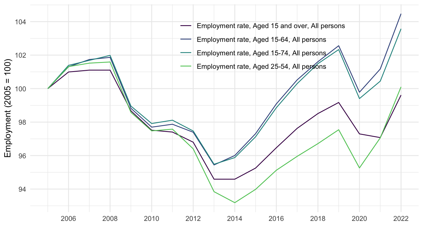
Men
Code
STLABOUR %>%
  filter(SUBJECT %in% c("LREMTTMA", "LREM25MA", "LREM64MA", "LREM74MA"),
         MEASURE == "ST",
         FREQUENCY == "A",
         LOCATION == "ITA") %>%
  left_join(STLABOUR_var$SUBJECT, by = "SUBJECT") %>%
  frequency_to_date %>%
  filter(date >= as.Date("2005-01-01")) %>%
  group_by(Subject) %>%
  mutate(obsValue = 100*obsValue/obsValue[date == as.Date("2005-01-01")]) %>%
  ggplot() + geom_line() + theme_minimal() +
  aes(x = date, y = obsValue, color = Subject) +
  scale_color_manual(values = viridis(5)[1:4]) +
  scale_x_date(breaks = seq(1920, 2100, 2) %>% paste0("-01-01") %>% as.Date,
               labels = date_format("%Y")) +
  theme(legend.position = c(0.6, 0.8),
        legend.title = element_blank()) +
  scale_y_continuous(breaks = seq(0, 200, 2)) +
  ylab("Employment (2005 = 100)") + xlab("")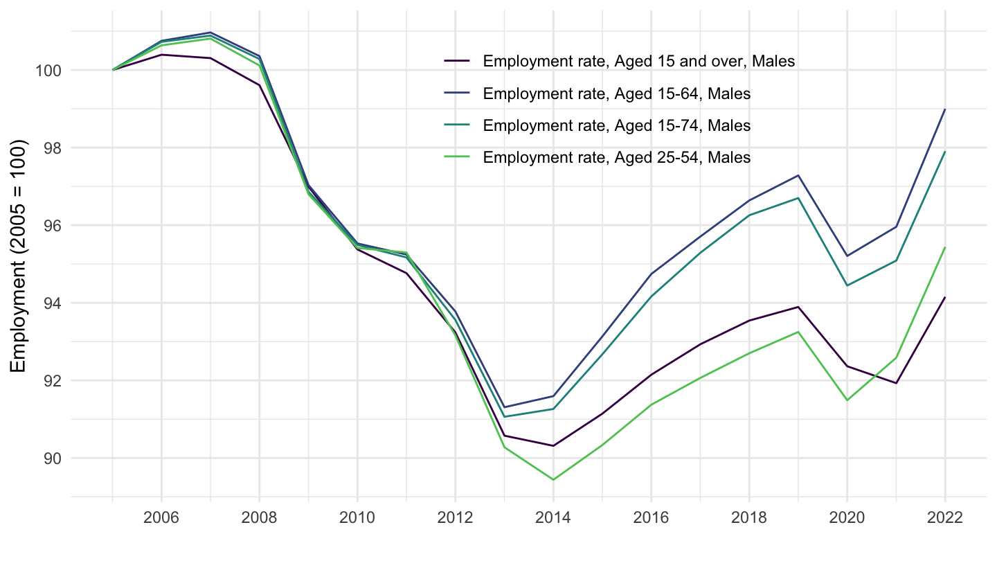
Etats-Unis, Zone Euro
France, Etats-Unis
All
Code
STLABOUR %>%
  # LRHUTTTT: Harmonised unemployment Rate (monthly), Total, All persons
  # ST: Level, rate or quantity series
  filter(SUBJECT %in% c("LREMTTTT", "LREM25TT", "LREM64TT", "LREM74TT"),
         MEASURE == "ST",
         FREQUENCY == "Q",
         LOCATION %in% c("FRA", "USA")) %>%
  left_join(STLABOUR_var$SUBJECT, by = "SUBJECT") %>%
  left_join(STLABOUR_var$LOCATION, by = "LOCATION") %>%
  frequency_to_date %>%
  ggplot() + geom_line() + theme_minimal() +
  aes(x = date, y = obsValue/100, linetype = Location, color = Subject) +
  scale_x_date(breaks = seq(1920, 2100, 5) %>% paste0("-01-01") %>% as.Date,
               labels = date_format("%Y")) +
  theme(legend.position = c(0.25, 0.8),
        legend.title = element_blank()) +
  scale_y_continuous(breaks = 0.01*seq(0, 80, 5),
                     labels = scales::percent_format(accuracy = 1)) +
  ylab("Employment Rate (%)") + xlab("")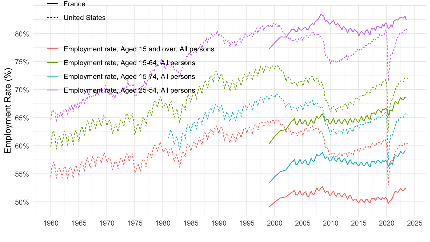
2000-
Code
STLABOUR %>%
  # LRHUTTTT: Harmonised unemployment Rate (monthly), Total, All persons
  # ST: Level, rate or quantity series
  filter(SUBJECT %in% c("LREMTTTT", "LREM25TT", "LREM64TT", "LREM74TT"),
         MEASURE == "ST",
         FREQUENCY == "Q",
         LOCATION %in% c("FRA", "USA")) %>%
  left_join(STLABOUR_var$SUBJECT, by = "SUBJECT") %>%
  left_join(STLABOUR_var$LOCATION, by = "LOCATION") %>%
  frequency_to_date %>%
  filter(date >= as.Date("1999-01-01")) %>%
  ggplot() + geom_line(aes(x = date, y = obsValue/100, linetype = Location, color = Subject)) +
  theme_minimal() +
  scale_x_date(breaks = seq(1920, 2100, 2) %>% paste0("-01-01") %>% as.Date,
               labels = date_format("%Y")) +
  scale_color_manual(values = rainbow(4)[1:4]) +
  scale_linetype_manual(values = c("solid", "dashed")) +
  theme(legend.position = "none") +
  annotate("text", x = as.Date("2021-07-01"), y = 0.8, label= "25-54", color = rainbow(4)[4]) +
  annotate("text", x = as.Date("2021-07-01"), y = 0.69, label= "15-64", color = rainbow(4)[2]) +
  annotate("text", x = as.Date("2021-07-01"), y = 0.62, label= "15-74", color = rainbow(4)[3]) +
  annotate("text", x = as.Date("2021-07-01"), y = 0.55, label= "15+", color = rainbow(4)[1]) +
  scale_y_continuous(breaks = 0.01*seq(0, 100, 5),
                     labels = scales::percent_format(accuracy = 1)) +
  ylab("Employment Rate (%)") + xlab("") +
  labs(caption = "Solid: France, Dotted: United States")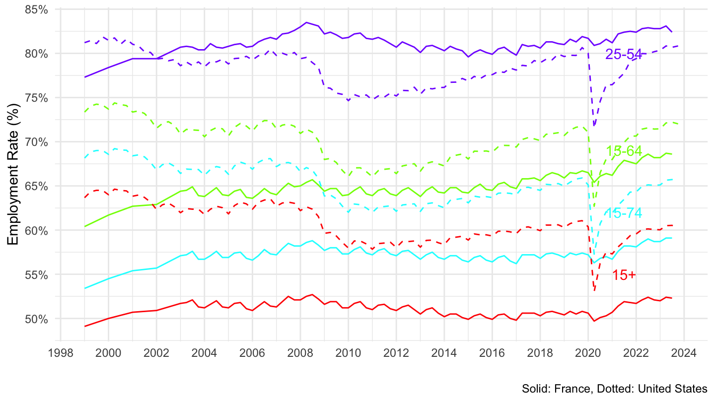
2017-
Code
STLABOUR %>%
  # LRHUTTTT: Harmonised unemployment Rate (monthly), Total, All persons
  # ST: Level, rate or quantity series
  filter(SUBJECT %in% c("LREMTTTT", "LREM25TT", "LREM64TT", "LREM74TT"),
         MEASURE == "ST",
         FREQUENCY == "Q",
         LOCATION %in% c("FRA", "USA")) %>%
  left_join(STLABOUR_var$SUBJECT, by = "SUBJECT") %>%
  left_join(STLABOUR_var$LOCATION, by = "LOCATION") %>%
  frequency_to_date %>%
  filter(date >= as.Date("2017-01-01")) %>%
  ggplot() + geom_line(aes(x = date, y = obsValue/100, linetype = Location, color = Subject)) +
  theme_minimal() +
  scale_x_date(breaks = seq(1920, 2100, 1) %>% paste0("-01-01") %>% as.Date,
               labels = date_format("%Y")) +
  scale_color_manual(values = rainbow(4)[1:4]) +
  scale_linetype_manual(values = c("solid", "dashed")) +
  theme(legend.position = "none") +
  annotate("text", x = as.Date("2021-07-01"), y = 0.8, label= "25-54", color = rainbow(4)[4]) +
  annotate("text", x = as.Date("2021-07-01"), y = 0.69, label= "15-64", color = rainbow(4)[2]) +
  annotate("text", x = as.Date("2021-07-01"), y = 0.62, label= "15-74", color = rainbow(4)[3]) +
  annotate("text", x = as.Date("2021-07-01"), y = 0.55, label= "15+", color = rainbow(4)[1]) +
  scale_y_continuous(breaks = 0.01*seq(0, 100, 5),
                     labels = scales::percent_format(accuracy = 1)) +
  ylab("Employment Rate (%)") + xlab("") +
  labs(caption = "Solid: France, Dotted: United States")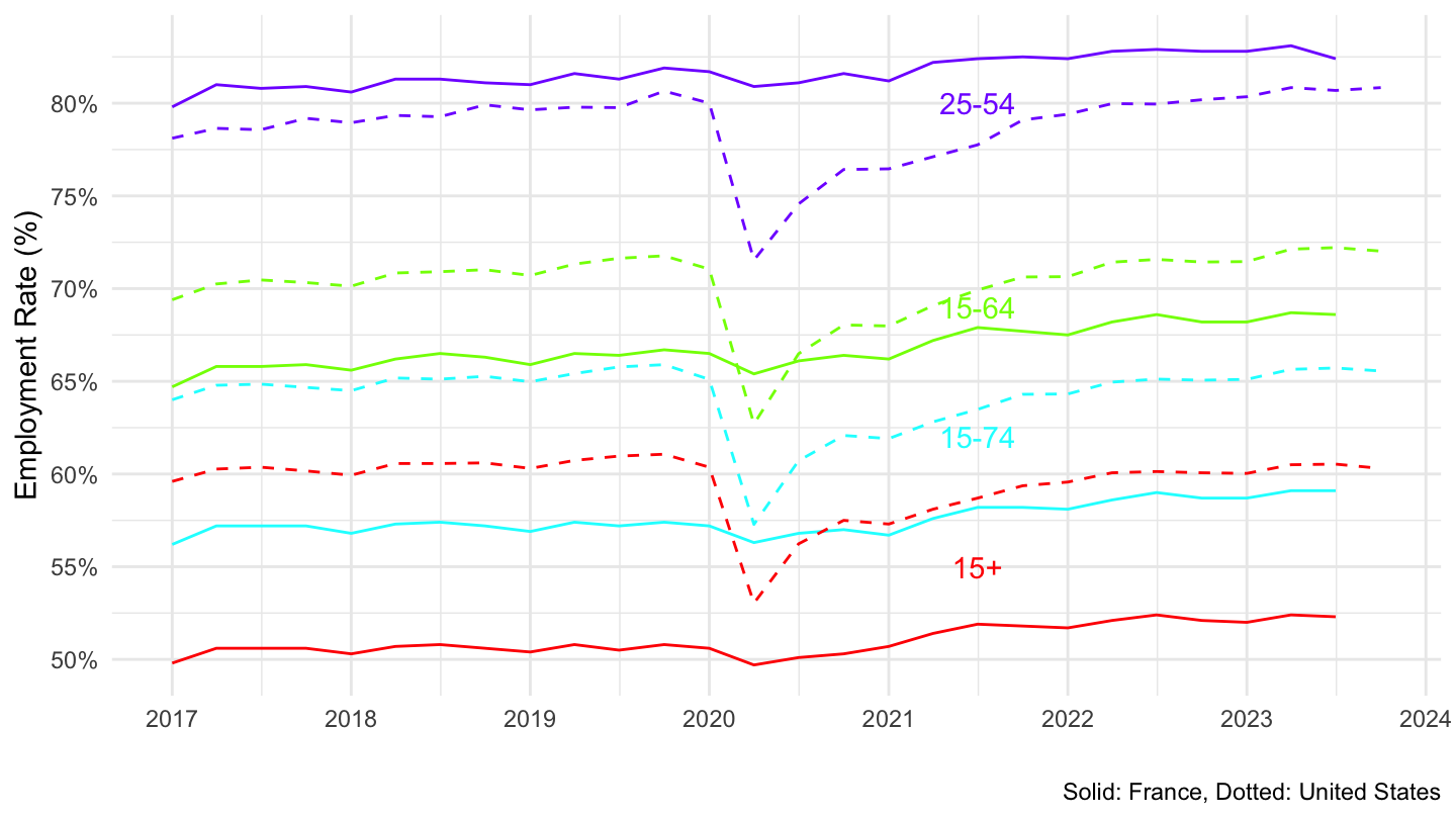
2019Q2-
Code
STLABOUR %>%
  # LRHUTTTT: Harmonised unemployment Rate (monthly), Total, All persons
  # ST: Level, rate or quantity series
  filter(SUBJECT %in% c("LREMTTTT", "LREM25TT", "LREM64TT", "LREM74TT"),
         MEASURE == "ST",
         FREQUENCY == "Q",
         LOCATION %in% c("FRA", "USA")) %>%
  left_join(STLABOUR_var$SUBJECT, by = "SUBJECT") %>%
  left_join(STLABOUR_var$LOCATION, by = "LOCATION") %>%
  frequency_to_date %>%
  filter(date >= as.Date("2019-04-01")) %>%
  mutate(obsValue = obsValue/100) %>%
  ggplot() + geom_line(aes(x = date, y = obsValue, linetype = Location, color = Subject)) +
  theme_minimal() + add_8flags +
  scale_x_date(breaks = "3 months",
               labels = date_format("%b %Y")) +
  scale_color_manual(values = rainbow(4)[1:4]) +
  scale_linetype_manual(values = c("solid", "dashed")) +
  annotate("text", x = as.Date("2021-07-01"), y = 0.8, label= "25-54", color = rainbow(4)[4]) +
  annotate("text", x = as.Date("2021-07-01"), y = 0.69, label= "15-64", color = rainbow(4)[2]) +
  annotate("text", x = as.Date("2021-07-01"), y = 0.62, label= "15-74", color = rainbow(4)[3]) +
  annotate("text", x = as.Date("2021-07-01"), y = 0.55, label= "15+", color = rainbow(4)[1]) +
  scale_y_continuous(breaks = 0.01*seq(0, 100, 5),
                     labels = scales::percent_format(accuracy = 1),
                     limits = c(0.45, 0.85)) +
  ylab("Employment Rate (%)") + xlab("") +
  theme(legend.position = "none",
        axis.text.x = element_text(angle = 45, vjust = 1, hjust = 1))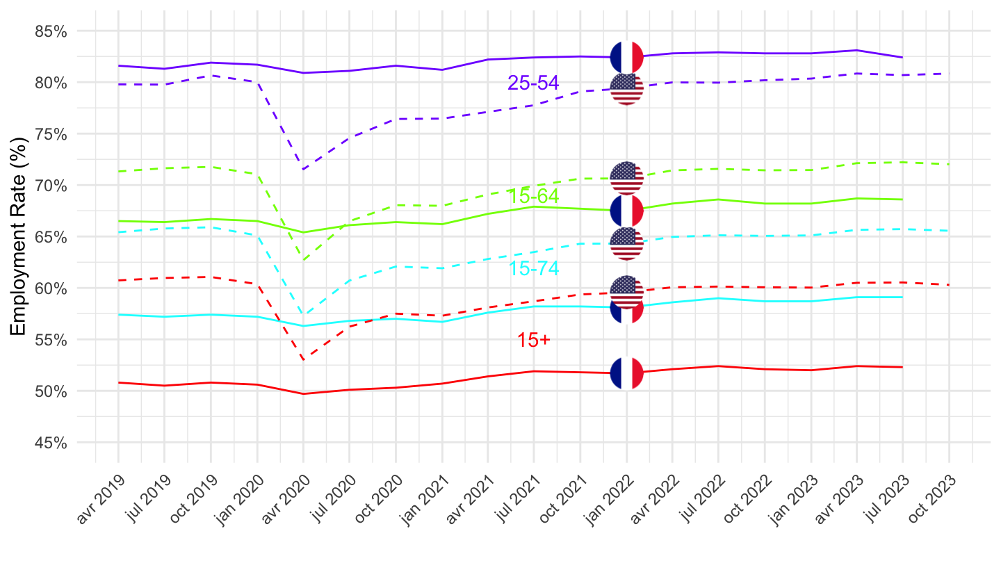
2019Q2-
Code
STLABOUR %>%
  # LRHUTTTT: Harmonised unemployment Rate (monthly), Total, All persons
  # ST: Level, rate or quantity series
  filter(SUBJECT %in% c("LREMTTTT", "LREM25TT", "LREM64TT", "LREM74TT"),
         MEASURE == "ST",
         FREQUENCY == "Q",
         LOCATION %in% c("FRA", "USA")) %>%
  left_join(STLABOUR_var$SUBJECT, by = "SUBJECT") %>%
  left_join(STLABOUR_var$LOCATION, by = "LOCATION") %>%
  frequency_to_date %>%
  filter(date >= as.Date("2019-04-01")) %>%
  mutate(obsValue = obsValue/100) %>%
  left_join(colors, by = c("Location" = "country")) %>%
  ggplot() + geom_line(aes(x = date, y = obsValue, linetype = Subject, color = color)) +
  theme_minimal() + add_8flags +
  scale_x_date(breaks = "3 months",
               labels = date_format("%b %Y")) +
  scale_color_identity() +
  scale_linetype_manual(values = c("solid", "dashed", "dotted", "solid")) +
  annotate("text", x = as.Date("2021-07-01"), y = 0.8, label= "25-54") +
  annotate("text", x = as.Date("2021-07-01"), y = 0.69, label= "15-64") +
  annotate("text", x = as.Date("2021-07-01"), y = 0.61, label= "15-74") +
  annotate("text", x = as.Date("2021-07-01"), y = 0.55, label= "15+") +
  scale_y_continuous(breaks = 0.01*seq(0, 100, 5),
                     labels = scales::percent_format(accuracy = 1),
                     limits = c(0.45, 0.85)) +
  ylab("Employment Rate (%)") + xlab("") +
  theme(legend.position = "none",
        axis.text.x = element_text(angle = 45, vjust = 1, hjust = 1))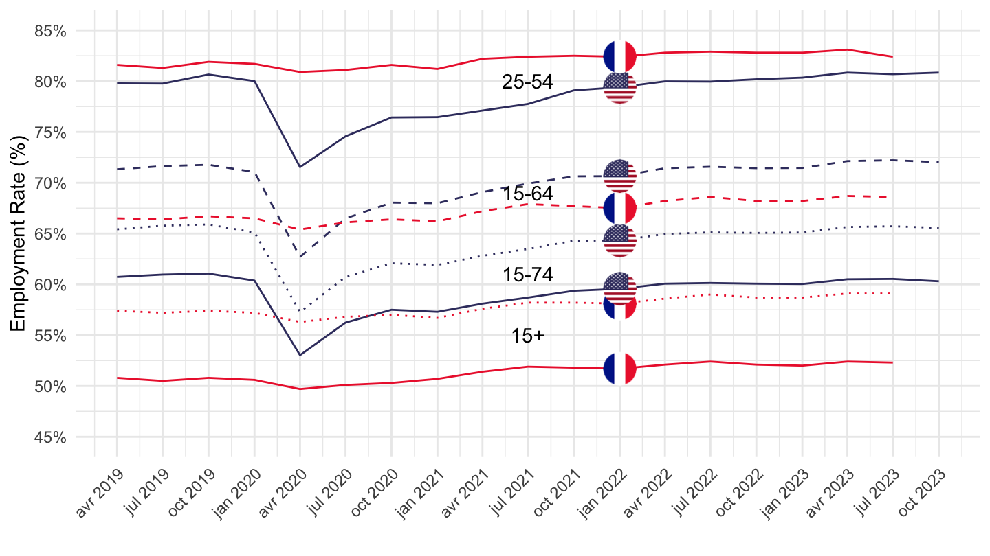
France
All
Code
STLABOUR %>%
  # LRHUTTTT: Harmonised unemployment Rate (monthly), Total, All persons
  # ST: Level, rate or quantity series
  filter(SUBJECT %in% c("LREMTTTT", "LREM25TT", "LREM64TT", "LREM74TT"),
         MEASURE == "ST",
         FREQUENCY == "A",
         LOCATION == "FRA") %>%
  left_join(STLABOUR_var$SUBJECT, by = "SUBJECT") %>%
  frequency_to_date %>%
  ggplot() + geom_line() + theme_minimal() +
  aes(x = date, y = obsValue/100, color = Subject) +
  scale_color_manual(values = viridis(5)[1:4]) +
  scale_x_date(breaks = seq(1920, 2100, 5) %>% paste0("-01-01") %>% as.Date,
               labels = date_format("%Y")) +
  theme(legend.position = c(0.6, 0.8),
        legend.title = element_blank()) +
  scale_y_continuous(breaks = 0.01*seq(0, 80, 5),
                     labels = scales::percent_format(accuracy = 1)) +
  ylab("Employment Rate (%)") + xlab("")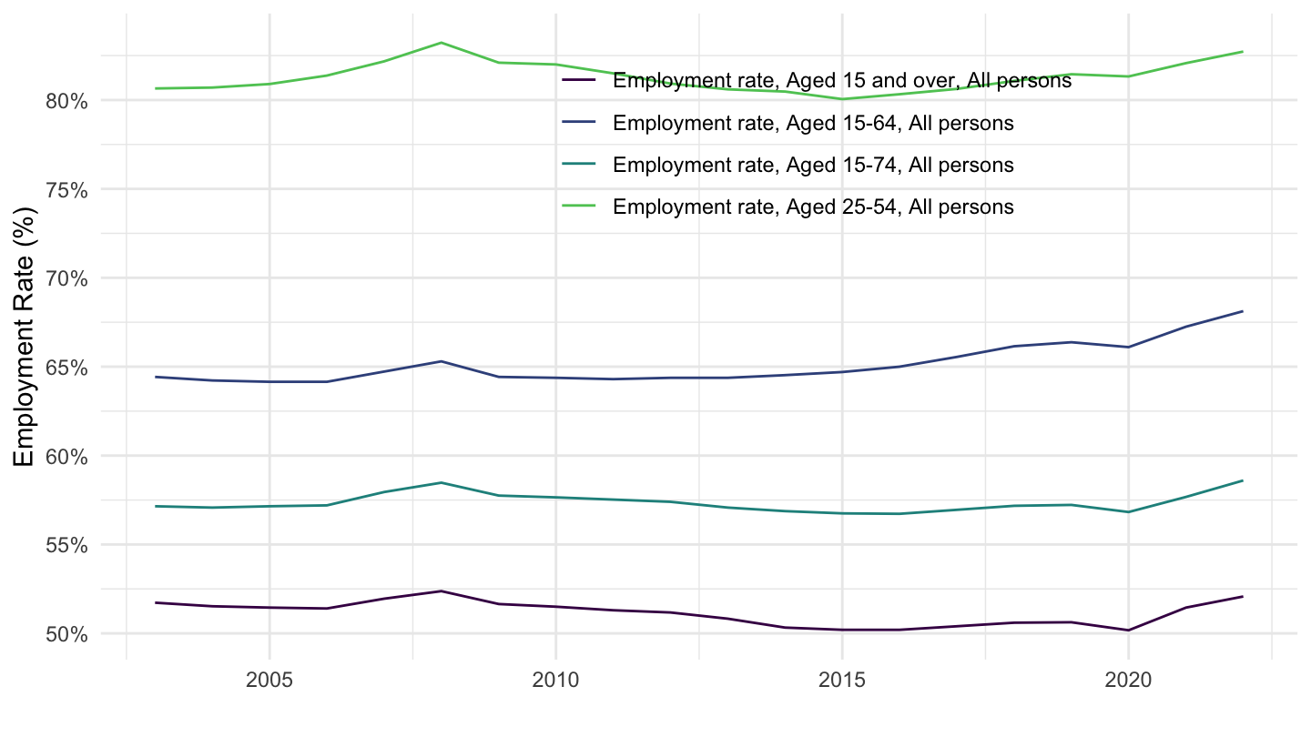
Men
Code
STLABOUR %>%
  filter(SUBJECT %in% c("LREMTTMA", "LREM25MA", "LREM64MA", "LREM74MA"),
         MEASURE == "ST",
         FREQUENCY == "A",
         LOCATION == "FRA") %>%
  left_join(STLABOUR_var$SUBJECT, by = "SUBJECT") %>%
  frequency_to_date %>%
  filter(date >= as.Date("2005-01-01")) %>%
  group_by(Subject) %>%
  mutate(obsValue = 100*obsValue/obsValue[date == as.Date("2005-01-01")]) %>%
  ggplot() + geom_line() + theme_minimal() +
  aes(x = date, y = obsValue, color = Subject) +
  scale_color_manual(values = viridis(5)[1:4]) +
  scale_x_date(breaks = seq(1920, 2100, 2) %>% paste0("-01-01") %>% as.Date,
               labels = date_format("%Y")) +
  theme(legend.position = c(0.6, 0.8),
        legend.title = element_blank()) +
  scale_y_continuous(breaks = seq(0, 200, 2)) +
  ylab("Employment (2005 = 100)") + xlab("")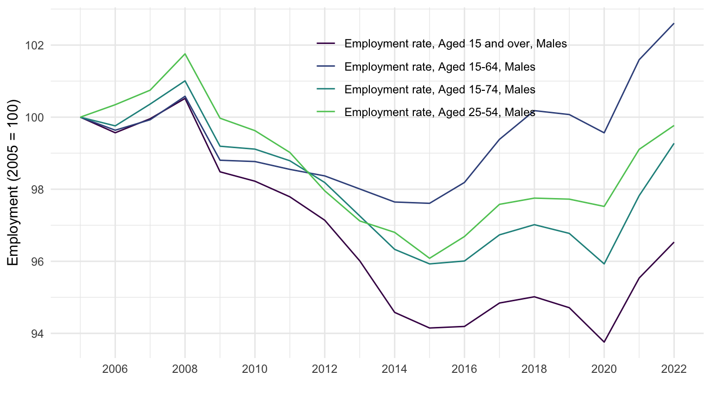
Germany
Code
STLABOUR %>%
  # LRHUTTTT: Harmonised unemployment Rate (monthly), Total, All persons
  # ST: Level, rate or quantity series
  filter(SUBJECT %in% c("LREMTTTT", "LREM25TT", "LREM64TT", "LREM74TT"),
         MEASURE == "ST",
         FREQUENCY == "A",
         LOCATION == "DEU") %>%
  left_join(STLABOUR_var$SUBJECT, by = "SUBJECT") %>%
  frequency_to_date %>%
  ggplot() + geom_line() + theme_minimal() +
  aes(x = date, y = obsValue/100, color = Subject) +
  scale_color_manual(values = viridis(5)[1:4]) +
  scale_x_date(breaks = seq(1920, 2100, 2) %>% paste0("-01-01") %>% as.Date,
               labels = date_format("%Y")) +
  theme(legend.position = c(0.6, 0.8),
        legend.title = element_blank()) +
  scale_y_continuous(breaks = 0.01*seq(0, 100, 5),
                     labels = scales::percent_format(accuracy = 1)) +
  ylab("Employment Rate (%)") + xlab("")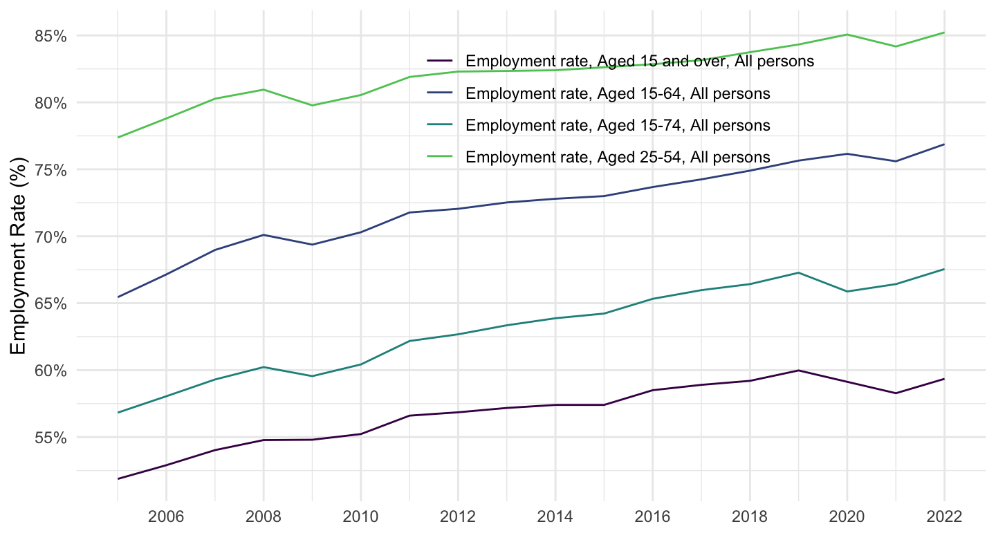
Men
Code
STLABOUR %>%
  filter(SUBJECT %in% c("LREMTTMA", "LREM25MA", "LREM64MA", "LREM74MA"),
         MEASURE == "ST",
         FREQUENCY == "A",
         LOCATION == "DEU") %>%
  left_join(STLABOUR_var$SUBJECT, by = "SUBJECT") %>%
  frequency_to_date %>%
  filter(date >= as.Date("2005-01-01")) %>%
  group_by(Subject) %>%
  mutate(obsValue = 100*obsValue/obsValue[date == as.Date("2005-01-01")]) %>%
  ggplot() + geom_line() + theme_minimal() +
  aes(x = date, y = obsValue, color = Subject) +
  scale_color_manual(values = viridis(5)[1:4]) +
  scale_x_date(breaks = seq(1920, 2100, 2) %>% paste0("-01-01") %>% as.Date,
               labels = date_format("%Y")) +
  theme(legend.position = c(0.3, 0.8),
        legend.title = element_blank()) +
  scale_y_continuous(breaks = seq(0, 200, 2)) +
  ylab("Employment (2005 = 100)") + xlab("")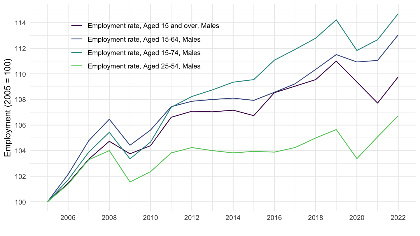
LREMTTTT - Employment rate, Aged 15 and over, All persons
Table
Code
STLABOUR %>%
  # LREMTTTT: Harmonised unemployment Rate (monthly), Total, All persons
  # ST: Level, rate or quantity series
  filter(SUBJECT == "LREMTTTT",
         MEASURE == "ST",
         FREQUENCY %in% c("Q", "M", "A")) %>%
  left_join(STLABOUR_var$LOCATION, by = "LOCATION") %>%
  left_join(STLABOUR_var$FREQUENCY, by = "FREQUENCY") %>%
  group_by(LOCATION, Location, Frequency) %>%
  summarise(Nobs = n()) %>%
  spread(Frequency, Nobs) %>%
  arrange(-Annual) %>%
  mutate(Flag = gsub(" ", "-", str_to_lower(Location)),
         Flag = paste0('<img src="../../icon/flag/vsmall/', Flag, '.png" alt="Flag">')) %>%
  select(Flag, everything()) %>%
  {if (is_html_output()) datatable(., filter = 'top', rownames = F, escape = F) else .}
Individual Countries: Different Frequencies
Iceland
Code
STLABOUR %>%
  # LRHUTTTT: Harmonised unemployment Rate (monthly), Total, All persons
  # ST: Level, rate or quantity series
  filter(SUBJECT %in% c("LRHUTTTT"),
         MEASURE == "ST",
         FREQUENCY %in% c("A", "M", "Q"),
         LOCATION == c("ISL")) %>%
  left_join(STLABOUR_var$FREQUENCY, by = "FREQUENCY") %>%
  frequency_to_date %>%
  ggplot() + geom_line() + theme_minimal() +
  aes(x = date, y = obsValue/100, color = Frequency) +
  scale_color_manual(values = viridis(4)[1:3]) +
  scale_x_date(breaks = seq(1920, 2100, 2) %>% paste0("-01-01") %>% as.Date,
               labels = date_format("%Y")) +
  theme(legend.position = c(0.2, 0.8),
        legend.title = element_blank()) +
  scale_y_continuous(breaks = 0.01*seq(-7, 80, 1),
                     labels = scales::percent_format(accuracy = 1)) +
  ylab("Unemployment Rate (%)") + xlab("")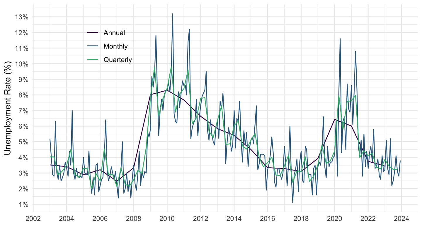
Japan
Code
STLABOUR %>%
  # LRHUTTTT: Harmonised unemployment Rate (monthly), Total, All persons
  # ST: Level, rate or quantity series
  filter(SUBJECT %in% c("LRHUTTTT"),
         MEASURE == "ST",
         FREQUENCY %in% c("A", "M", "Q"),
         LOCATION == c("JPN")) %>%
  left_join(STLABOUR_var$FREQUENCY, by = "FREQUENCY") %>%
  frequency_to_date %>%
  ggplot() + geom_line() + theme_minimal() +
  aes(x = date, y = obsValue/100, color = Frequency) +
  scale_color_manual(values = viridis(4)[1:3]) +
  scale_x_date(breaks = seq(1920, 2100, 5) %>% paste0("-01-01") %>% as.Date,
               labels = date_format("%Y")) +
  theme(legend.position = c(0.2, 0.8),
        legend.title = element_blank()) +
  scale_y_continuous(breaks = 0.01*seq(-7, 80, 1),
                     labels = scales::percent_format(accuracy = 1)) +
  ylab("Unemployment Rate (%)") + xlab("")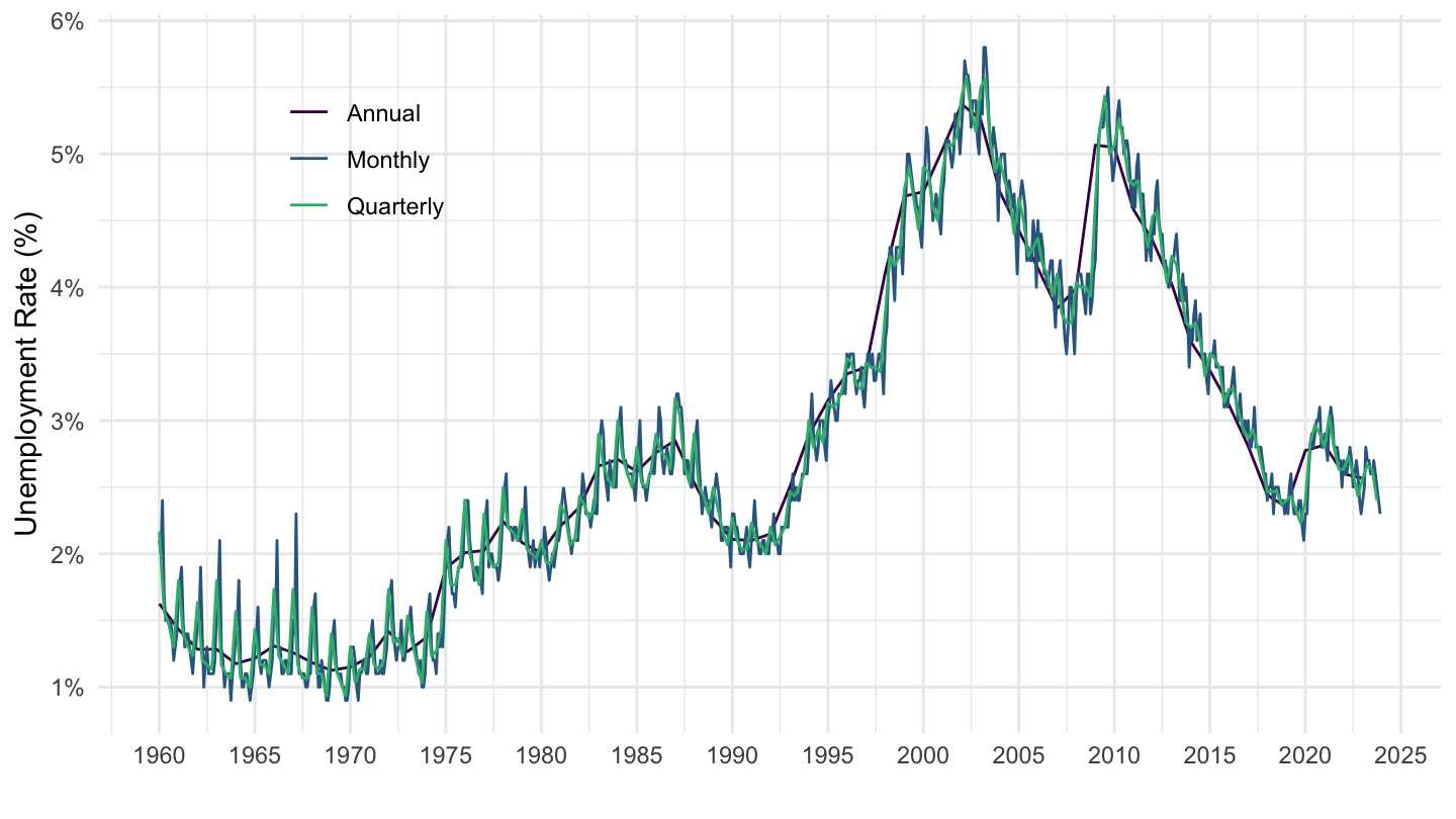
United States
Code
STLABOUR %>%
  # LRHUTTTT: Harmonised unemployment Rate (monthly), Total, All persons
  # ST: Level, rate or quantity series
  filter(SUBJECT %in% c("LRHUTTTT"),
         MEASURE == "ST",
         FREQUENCY %in% c("A", "M", "Q"),
         LOCATION == c("USA")) %>%
  left_join(STLABOUR_var$FREQUENCY, by = "FREQUENCY") %>%
  frequency_to_date %>%
  ggplot() + geom_line() + theme_minimal() +
  aes(x = date, y = obsValue/100, color = Frequency) +
  scale_color_manual(values = viridis(4)[1:3]) +
  scale_x_date(breaks = seq(1920, 2100, 5) %>% paste0("-01-01") %>% as.Date,
               labels = date_format("%Y")) +
  theme(legend.position = c(0.2, 0.8),
        legend.title = element_blank()) +
  scale_y_continuous(breaks = 0.01*seq(-7, 80, 1),
                     labels = scales::percent_format(accuracy = 1)) +
  ylab("Unemployment Rate (%)") + xlab("")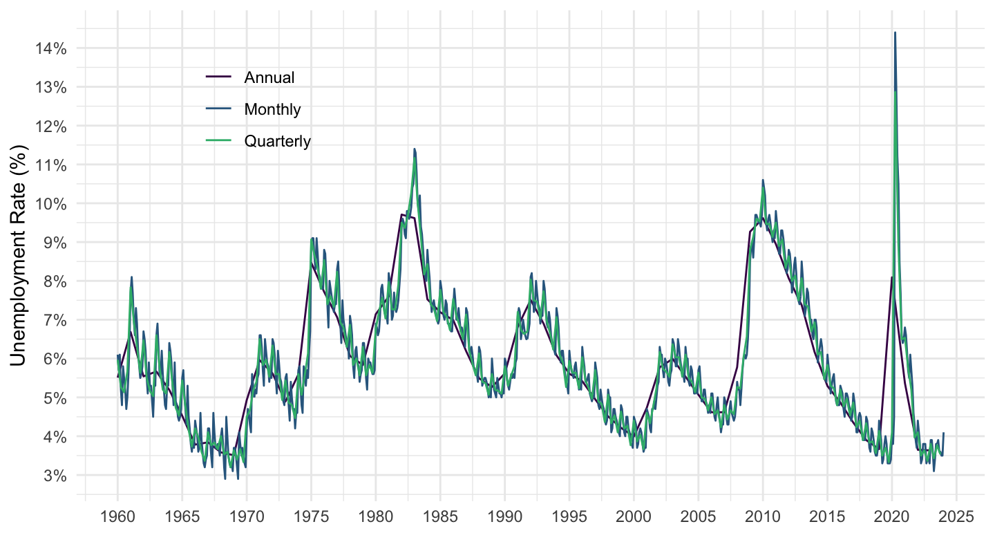
Australia
All
Code
STLABOUR %>%
  # LRHUTTTT: Harmonised unemployment Rate (monthly), Total, All persons
  # ST: Level, rate or quantity series
  filter(SUBJECT %in% c("LRHUTTTT"),
         MEASURE == "ST",
         FREQUENCY %in% c("A", "M", "Q"),
         LOCATION == c("AUS")) %>%
  left_join(STLABOUR_var$FREQUENCY, by = "FREQUENCY") %>%
  frequency_to_date %>%
  ggplot() + geom_line() + theme_minimal() +
  aes(x = date, y = obsValue/100, color = Frequency) +
  scale_color_manual(values = viridis(4)[1:3]) +
  scale_x_date(breaks = seq(1920, 2100, 5) %>% paste0("-01-01") %>% as.Date,
               labels = date_format("%Y")) +
  theme(legend.position = c(0.8, 0.8),
        legend.title = element_blank()) +
  scale_y_continuous(breaks = 0.01*seq(-7, 80, 1),
                     labels = scales::percent_format(accuracy = 1)) +
  ylab("Unemployment Rate (%)") + xlab("")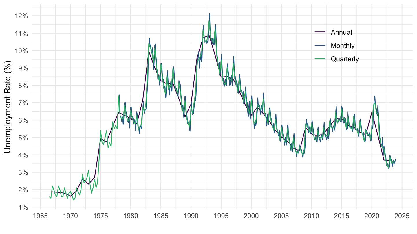
1990-
Code
STLABOUR %>%
  # LRHUTTTT: Harmonised unemployment Rate (monthly), Total, All persons
  # ST: Level, rate or quantity series
  filter(SUBJECT %in% c("LRHUTTTT"),
         MEASURE == "ST",
         FREQUENCY %in% c("A", "M", "Q"),
         LOCATION == c("AUS")) %>%
  left_join(STLABOUR_var$FREQUENCY, by = "FREQUENCY") %>%
  frequency_to_date %>%
  filter(date >= as.Date("1990-01-01")) %>%
  ggplot() + geom_line() + theme_minimal() +
  aes(x = date, y = obsValue/100, color = Frequency) +
  scale_color_manual(values = viridis(4)[1:3]) +
  scale_x_date(breaks = seq(1920, 2100, 5) %>% paste0("-01-01") %>% as.Date,
               labels = date_format("%Y")) +
  theme(legend.position = c(0.8, 0.8),
        legend.title = element_blank()) +
  scale_y_continuous(breaks = 0.01*seq(-7, 80, 1),
                     labels = scales::percent_format(accuracy = 1)) +
  ylab("Unemployment Rate (%)") + xlab("")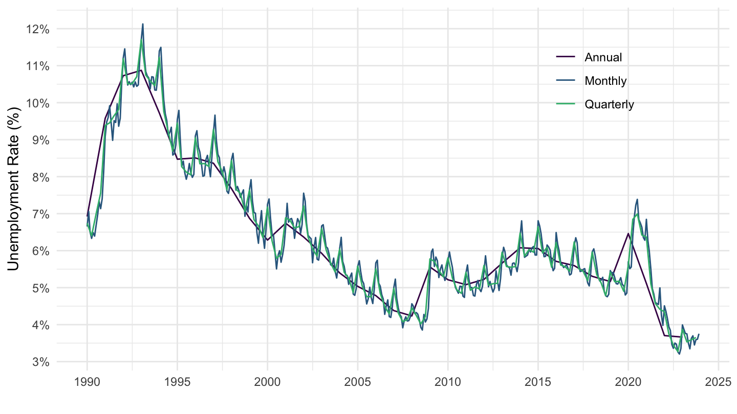
2010-
Code
STLABOUR %>%
  # LRHUTTTT: Harmonised unemployment Rate (monthly), Total, All persons
  # ST: Level, rate or quantity series
  filter(SUBJECT %in% c("LRHUTTTT"),
         MEASURE == "ST",
         FREQUENCY %in% c("A", "M", "Q"),
         LOCATION == c("AUS")) %>%
  left_join(STLABOUR_var$FREQUENCY, by = "FREQUENCY") %>%
  frequency_to_date %>%
  filter(date >= as.Date("2010-01-01")) %>%
  ggplot() + geom_line() + theme_minimal() +
  aes(x = date, y = obsValue/100, color = Frequency) +
  scale_color_manual(values = viridis(4)[1:3]) +
  scale_x_date(breaks = seq(1920, 2100, 1) %>% paste0("-01-01") %>% as.Date,
               labels = date_format("%Y")) +
  theme(legend.position = c(0.8, 0.8),
        legend.title = element_blank()) +
  scale_y_continuous(breaks = 0.01*seq(-7, 80, 0.5),
                     labels = scales::percent_format(accuracy = 0.1)) +
  ylab("Unemployment Rate (%)") + xlab("")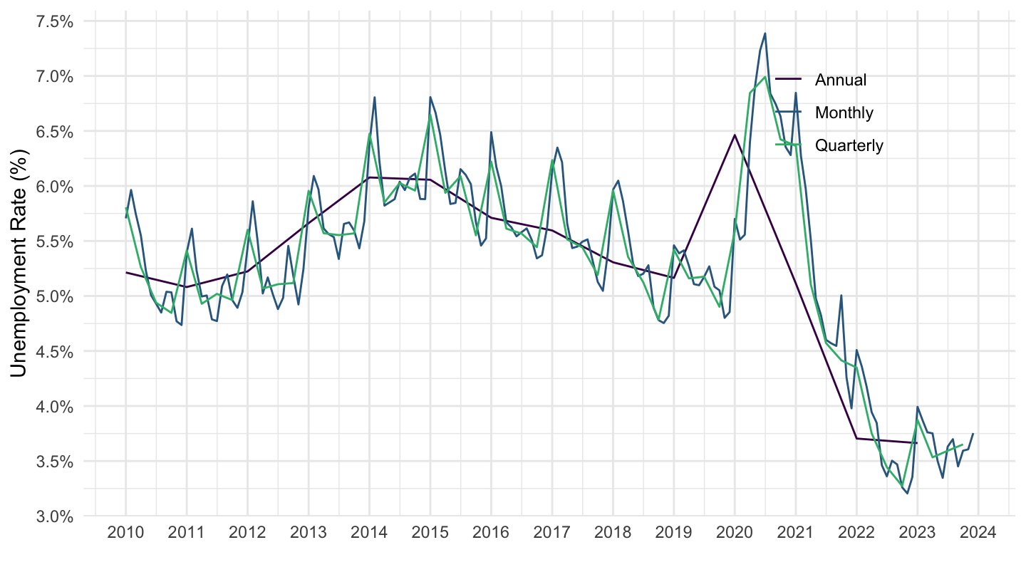
France
Code
STLABOUR %>%
  # LRHUTTTT: Harmonised unemployment Rate (monthly), Total, All persons
  # ST: Level, rate or quantity series
  filter(SUBJECT %in% c("LRHUTTTT"),
         MEASURE == "ST",
         FREQUENCY %in% c("A", "M", "Q"),
         LOCATION == c("FRA")) %>%
  left_join(STLABOUR_var$FREQUENCY, by = "FREQUENCY") %>%
  frequency_to_date %>%
  ggplot() + geom_line() + theme_minimal() +
  aes(x = date, y = obsValue/100, color = Frequency) +
  scale_color_manual(values = viridis(4)[1:3]) +
  scale_x_date(breaks = seq(1920, 2100, 5) %>% paste0("-01-01") %>% as.Date,
               labels = date_format("%Y")) +
  theme(legend.position = c(0.8, 0.8),
        legend.title = element_blank()) +
  scale_y_continuous(breaks = 0.01*seq(-7, 80, 1),
                     labels = scales::percent_format(accuracy = 1)) +
  ylab("Unemployment Rate (%)") + xlab("")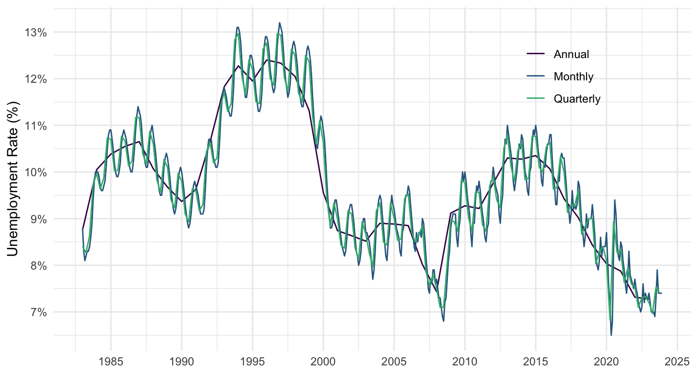
Canada
Code
STLABOUR %>%
  # LRHUTTTT: Harmonised unemployment Rate (monthly), Total, All persons
  # ST: Level, rate or quantity series
  filter(SUBJECT %in% c("LRHUTTTT"),
         MEASURE == "ST",
         FREQUENCY %in% c("A", "M", "Q"),
         LOCATION == c("CAN")) %>%
  left_join(STLABOUR_var$FREQUENCY, by = "FREQUENCY") %>%
  frequency_to_date %>%
  ggplot() + geom_line() + theme_minimal() +
  aes(x = date, y = obsValue/100, color = Frequency) +
  scale_color_manual(values = viridis(4)[1:3]) +
  scale_x_date(breaks = seq(1920, 2100, 5) %>% paste0("-01-01") %>% as.Date,
               labels = date_format("%Y")) +
  theme(legend.position = c(0.8, 0.8),
        legend.title = element_blank()) +
  scale_y_continuous(breaks = 0.01*seq(-7, 80, 1),
                     labels = scales::percent_format(accuracy = 1)) +
  ylab("Unemployment Rate (%)") + xlab("")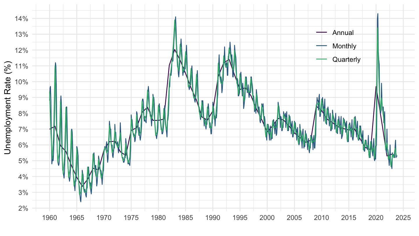
Korea
Code
STLABOUR %>%
  # LRHUTTTT: Harmonised unemployment Rate (monthly), Total, All persons
  # ST: Level, rate or quantity series
  filter(SUBJECT %in% c("LRHUTTTT"),
         MEASURE == "ST",
         FREQUENCY %in% c("A", "M", "Q"),
         LOCATION == c("KOR")) %>%
  left_join(STLABOUR_var$FREQUENCY, by = "FREQUENCY") %>%
  frequency_to_date %>%
  ggplot() + geom_line() + theme_minimal() +
  aes(x = date, y = obsValue/100, color = Frequency) +
  scale_color_manual(values = viridis(4)[1:3]) +
  scale_x_date(breaks = seq(1920, 2100, 5) %>% paste0("-01-01") %>% as.Date,
               labels = date_format("%Y")) +
  theme(legend.position = c(0.8, 0.8),
        legend.title = element_blank()) +
  scale_y_continuous(breaks = 0.01*seq(-7, 80, 1),
                     labels = scales::percent_format(accuracy = 1)) +
  ylab("Unemployment Rate (%)") + xlab("")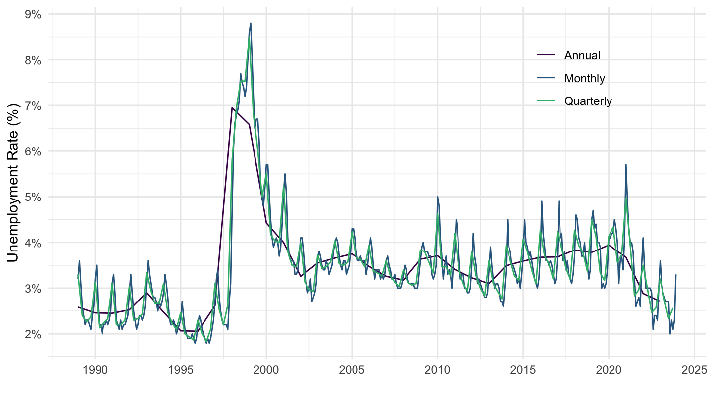
New Zealand
Code
STLABOUR %>%
  # LRHUTTTT: Harmonised unemployment Rate (monthly), Total, All persons
  # ST: Level, rate or quantity series
  filter(SUBJECT %in% c("LRHUTTTT"),
         MEASURE == "ST",
         FREQUENCY %in% c("A", "M", "Q"),
         LOCATION == c("NZL")) %>%
  left_join(STLABOUR_var$FREQUENCY, by = "FREQUENCY") %>%
  frequency_to_date %>%
  ggplot() + geom_line() + theme_minimal() +
  aes(x = date, y = obsValue/100, color = Frequency) +
  scale_color_manual(values = viridis(4)[1:3]) +
  scale_x_date(breaks = seq(1920, 2100, 5) %>% paste0("-01-01") %>% as.Date,
               labels = date_format("%Y")) +
  theme(legend.position = c(0.8, 0.8),
        legend.title = element_blank()) +
  scale_y_continuous(breaks = 0.01*seq(-7, 80, 1),
                     labels = scales::percent_format(accuracy = 1)) +
  ylab("Unemployment Rate (%)") + xlab("")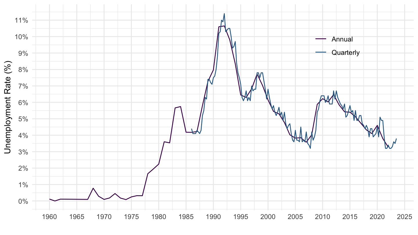
Belgium
Code
STLABOUR %>%
  # LRHUTTTT: Harmonised unemployment Rate (monthly), Total, All persons
  # ST: Level, rate or quantity series
  filter(SUBJECT %in% c("LRHUTTTT"),
         MEASURE == "ST",
         FREQUENCY %in% c("A", "M", "Q"),
         LOCATION == c("BEL")) %>%
  left_join(STLABOUR_var$FREQUENCY, by = "FREQUENCY") %>%
  frequency_to_date %>%
  ggplot() + geom_line() + theme_minimal() +
  aes(x = date, y = obsValue/100, color = Frequency) +
  scale_color_manual(values = viridis(4)[1:3]) +
  scale_x_date(breaks = seq(1920, 2100, 5) %>% paste0("-01-01") %>% as.Date,
               labels = date_format("%Y")) +
  theme(legend.position = c(0.8, 0.8),
        legend.title = element_blank()) +
  scale_y_continuous(breaks = 0.01*seq(-7, 80, 1),
                     labels = scales::percent_format(accuracy = 1)) +
  ylab("Unemployment Rate (%)") + xlab("")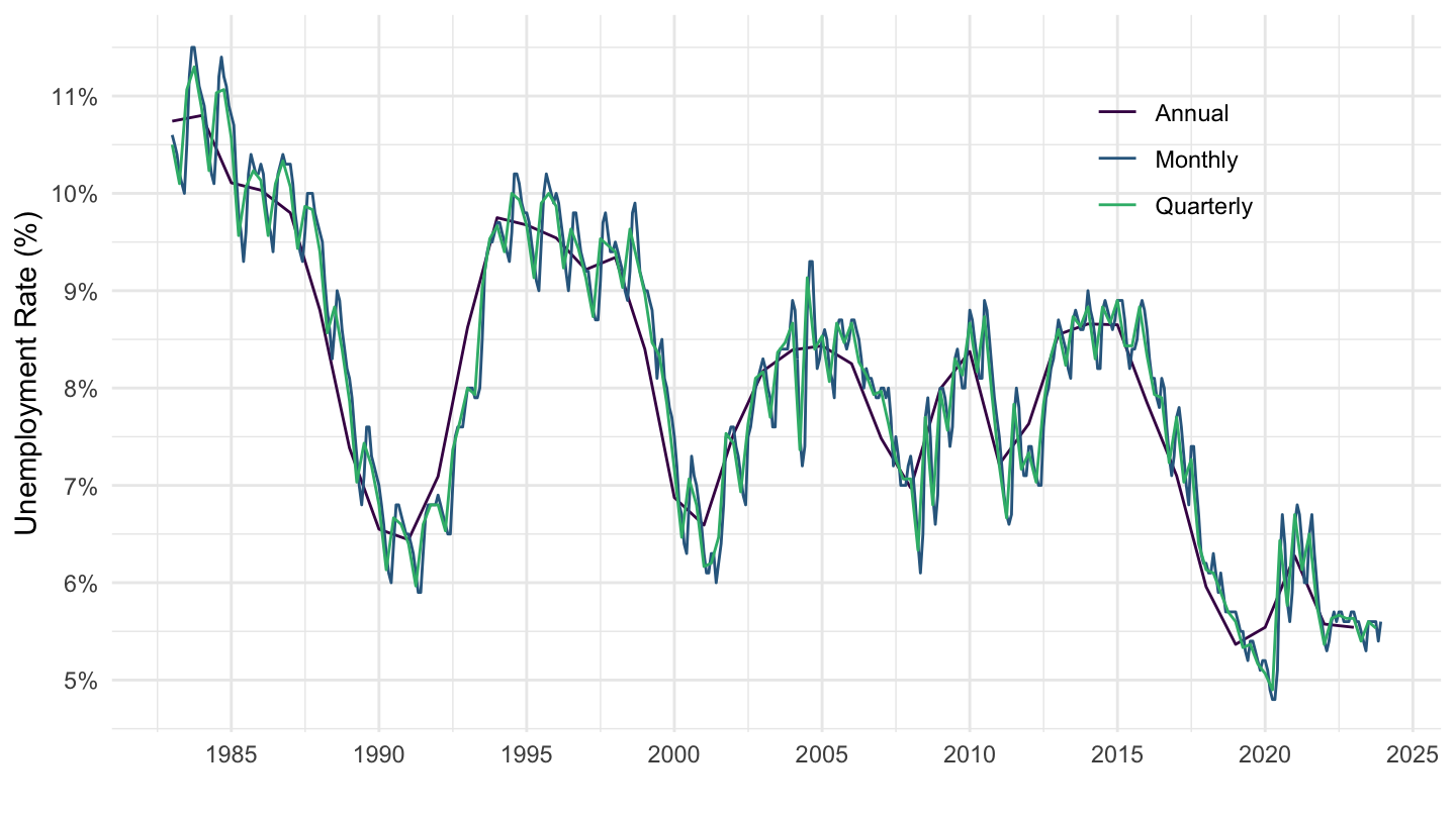
Denmark
Code
STLABOUR %>%
  # LRHUTTTT: Harmonised unemployment Rate (monthly), Total, All persons
  # ST: Level, rate or quantity series
  filter(SUBJECT %in% c("LRHUTTTT"),
         MEASURE == "ST",
         FREQUENCY %in% c("A", "M", "Q"),
         LOCATION == c("DNK")) %>%
  left_join(STLABOUR_var$FREQUENCY, by = "FREQUENCY") %>%
  frequency_to_date %>%
  ggplot() + geom_line() + theme_minimal() +
  aes(x = date, y = obsValue/100, color = Frequency) +
  scale_color_manual(values = viridis(4)[1:3]) +
  scale_x_date(breaks = seq(1920, 2100, 5) %>% paste0("-01-01") %>% as.Date,
               labels = date_format("%Y")) +
  theme(legend.position = c(0.8, 0.8),
        legend.title = element_blank()) +
  scale_y_continuous(breaks = 0.01*seq(-7, 80, 1),
                     labels = scales::percent_format(accuracy = 1)) +
  ylab("Unemployment Rate (%)") + xlab("")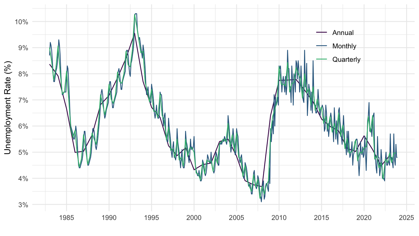
Austria
Code
STLABOUR %>%
  # LRHUTTTT: Harmonised unemployment Rate (monthly), Total, All persons
  # ST: Level, rate or quantity series
  filter(SUBJECT %in% c("LRHUTTTT"),
         MEASURE == "ST",
         FREQUENCY %in% c("A", "M", "Q"),
         LOCATION == c("AUT")) %>%
  left_join(STLABOUR_var$FREQUENCY, by = "FREQUENCY") %>%
  frequency_to_date %>%
  ggplot() + geom_line() + theme_minimal() +
  aes(x = date, y = obsValue/100, color = Frequency) +
  scale_color_manual(values = viridis(4)[1:3]) +
  scale_x_date(breaks = seq(1920, 2100, 5) %>% paste0("-01-01") %>% as.Date,
               labels = date_format("%Y")) +
  theme(legend.position = c(0.8, 0.2),
        legend.title = element_blank()) +
  scale_y_continuous(breaks = 0.01*seq(-7, 80, 1),
                     labels = scales::percent_format(accuracy = 1)) +
  ylab("Unemployment Rate (%)") + xlab("")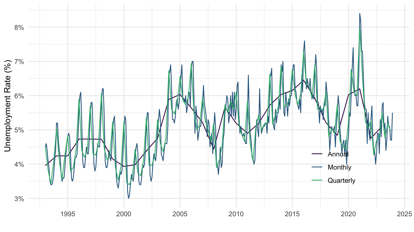
United Kingdom
Code
STLABOUR %>%
  # LRHUTTTT: Harmonised unemployment Rate (monthly), Total, All persons
  # ST: Level, rate or quantity series
  filter(SUBJECT %in% c("LRHUTTTT"),
         MEASURE == "ST",
         FREQUENCY %in% c("A", "M", "Q"),
         LOCATION == c("GBR")) %>%
  left_join(STLABOUR_var$FREQUENCY, by = "FREQUENCY") %>%
  frequency_to_date %>%
  ggplot() + geom_line() + theme_minimal() +
  aes(x = date, y = obsValue/100, color = Frequency) +
  scale_color_manual(values = viridis(4)[1:3]) +
  scale_x_date(breaks = seq(1920, 2100, 5) %>% paste0("-01-01") %>% as.Date,
               labels = date_format("%Y")) +
  theme(legend.position = c(0.8, 0.8),
        legend.title = element_blank()) +
  scale_y_continuous(breaks = 0.01*seq(-7, 80, 1),
                     labels = scales::percent_format(accuracy = 1)) +
  ylab("Unemployment Rate (%)") + xlab("")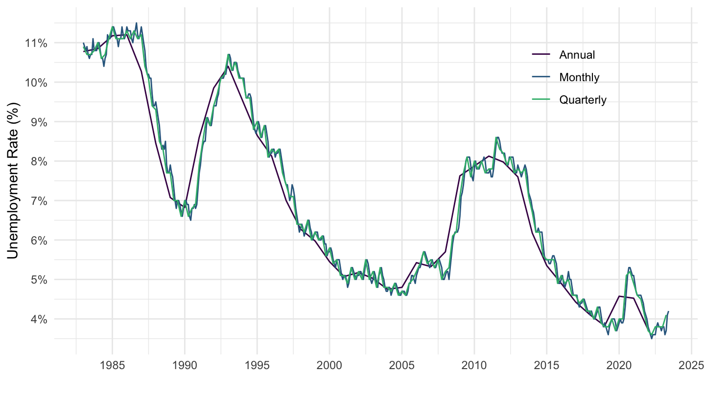
Individual Countries: Different Ages
Australia
Annual
Code
STLABOUR %>%
  # LRHUTTTT: Harmonised unemployment Rate (monthly), Total, All persons
  # ST: Level, rate or quantity series
  filter(SUBJECT %in% c("LRHUTTTT","LRUN64TT", "LRUN25TT"),
         MEASURE == "ST",
         FREQUENCY == "A",
         LOCATION == c("AUS")) %>%
  left_join(STLABOUR_var$SUBJECT, by = "SUBJECT") %>%
  frequency_to_date %>%
  ggplot() + geom_line() + theme_minimal() +
  aes(x = date, y = obsValue/100, color = Subject) +
  scale_color_manual(values = viridis(4)[1:3]) +
  scale_x_date(breaks = seq(1920, 2100, 5) %>% paste0("-01-01") %>% as.Date,
               labels = date_format("%Y")) +
  theme(legend.position = c(0.75, 0.9),
        legend.title = element_blank()) +
  scale_y_continuous(breaks = 0.01*seq(-7, 80, 1),
                     labels = scales::percent_format(accuracy = 1)) +
  ylab("Unemployment Rate (%)") + xlab("")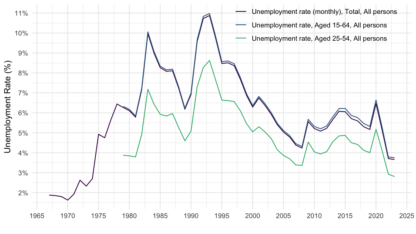
Monthly
Code
STLABOUR %>%
  # LRHUTTTT: Harmonised unemployment Rate (monthly), Total, All persons
  # ST: Level, rate or quantity series
  filter(SUBJECT %in% c("LRHUTTTT","LRUN64TT", "LRUN25TT"),
         MEASURE == "ST",
         FREQUENCY == "M",
         LOCATION == c("AUS")) %>%
  left_join(STLABOUR_var$SUBJECT, by = "SUBJECT") %>%
  frequency_to_date %>%
  ggplot() + geom_line() + theme_minimal() +
  aes(x = date, y = obsValue/100, color = Subject) +
  scale_color_manual(values = viridis(4)[1:3]) +
  scale_x_date(breaks = seq(1920, 2100, 5) %>% paste0("-01-01") %>% as.Date,
               labels = date_format("%Y")) +
  theme(legend.position = c(0.7, 0.8),
        legend.title = element_blank()) +
  scale_y_continuous(breaks = 0.01*seq(-7, 80, 1),
                     labels = scales::percent_format(accuracy = 1)) +
  ylab("Unemployment Rate (%)") + xlab("")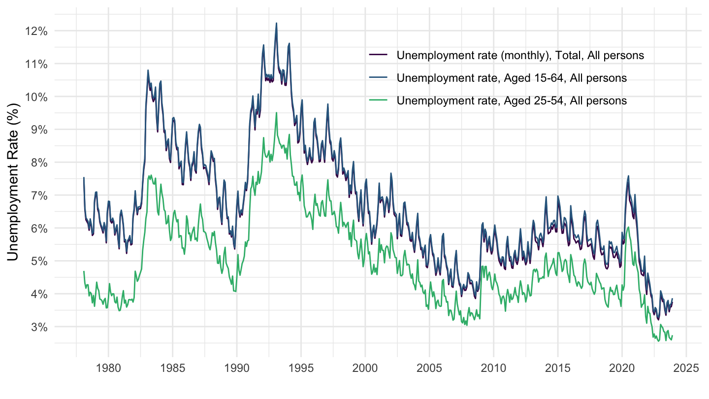
Iceland
Annual
Code
STLABOUR %>%
  # LRHUTTTT: Harmonised unemployment Rate (monthly), Total, All persons
  # ST: Level, rate or quantity series
  filter(SUBJECT %in% c("LRHUTTTT","LRUN64TT", "LRUN25TT"),
         MEASURE == "ST",
         FREQUENCY == "A",
         LOCATION == c("ISL")) %>%
  left_join(STLABOUR_var$SUBJECT, by = "SUBJECT") %>%
  frequency_to_date %>%
  ggplot() + geom_line() + theme_minimal() +
  aes(x = date, y = obsValue/100, color = Subject) +
  scale_color_manual(values = viridis(4)[1:3]) +
  scale_x_date(breaks = seq(1920, 2100, 2) %>% paste0("-01-01") %>% as.Date,
               labels = date_format("%Y")) +
  theme(legend.position = c(0.75, 0.9),
        legend.title = element_blank()) +
  scale_y_continuous(breaks = 0.01*seq(-7, 80, 1),
                     labels = scales::percent_format(accuracy = 1)) +
  ylab("Unemployment Rate (%)") + xlab("")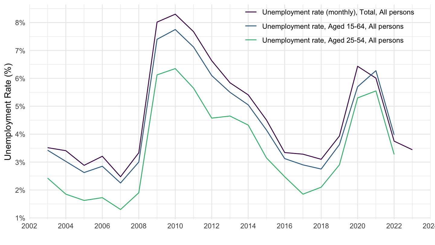
Monthly
Code
STLABOUR %>%
  # LRHUTTTT: Harmonised unemployment Rate (monthly), Total, All persons
  # ST: Level, rate or quantity series
  filter(SUBJECT %in% c("LRHUTTTT","LRUN64TT", "LRUN25TT"),
         MEASURE == "ST",
         FREQUENCY == "M",
         LOCATION == c("ISL")) %>%
  left_join(STLABOUR_var$SUBJECT, by = "SUBJECT") %>%
  frequency_to_date %>%
  ggplot() + geom_line() + theme_minimal() +
  aes(x = date, y = obsValue/100, color = Subject) +
  scale_color_manual(values = viridis(4)[1:3]) +
  scale_x_date(breaks = seq(1920, 2100, 5) %>% paste0("-01-01") %>% as.Date,
               labels = date_format("%Y")) +
  theme(legend.position = c(0.7, 0.8),
        legend.title = element_blank()) +
  scale_y_continuous(breaks = 0.01*seq(-7, 80, 1),
                     labels = scales::percent_format(accuracy = 1)) +
  ylab("Unemployment Rate (%)") + xlab("")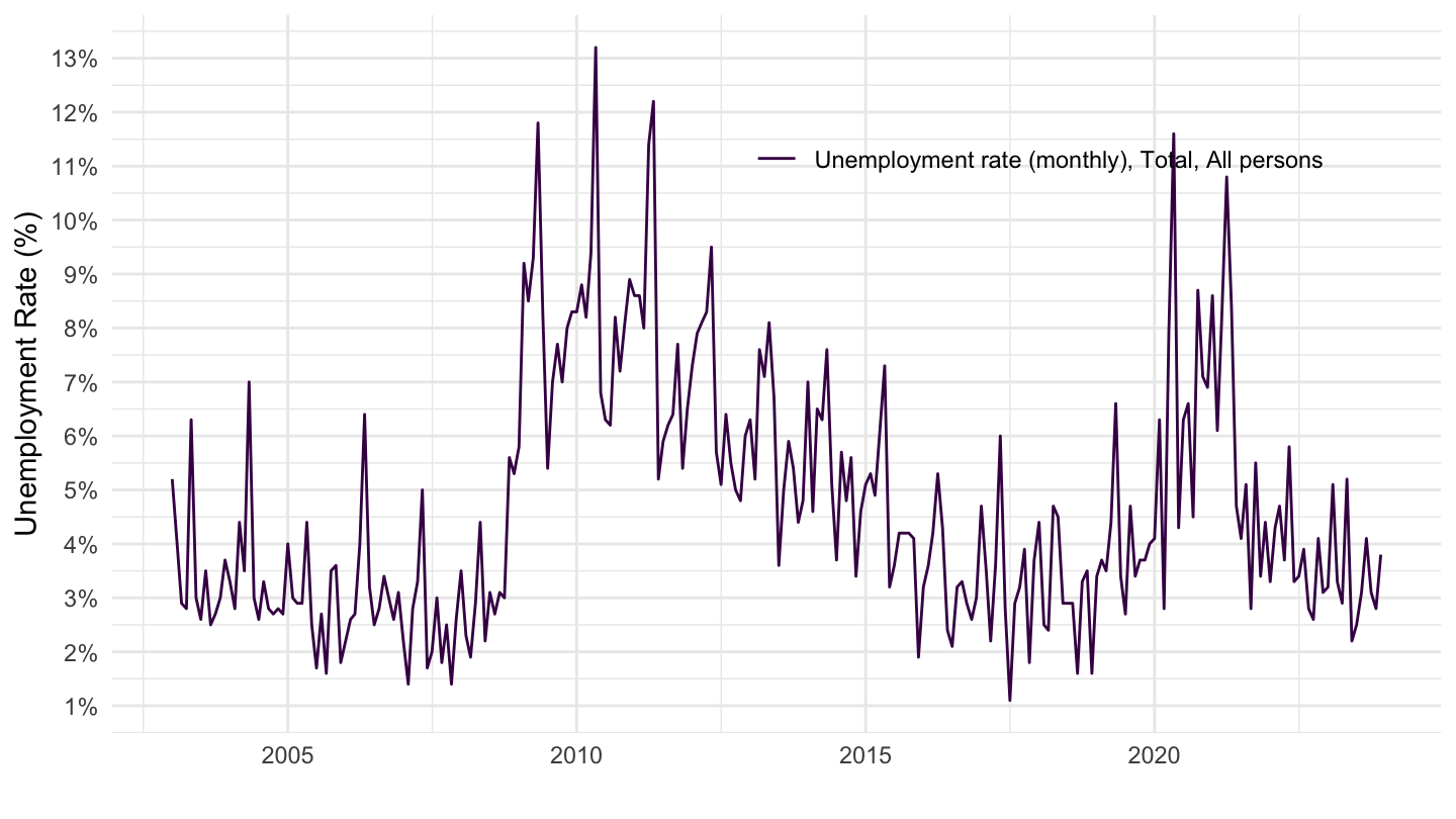
Harmonised unemployment Rate, Total, All persons - LRHUTTTT
Number of Obs - Annual, Quarterly, Monthly
Code
STLABOUR %>%
  # LRHUTTTT: Harmonised unemployment Rate (monthly), Total, All persons
  # ST: Level, rate or quantity series
  filter(SUBJECT == "LRHUTTTT",
         MEASURE == "ST",
         FREQUENCY %in% c("Q", "M", "A")) %>%
  left_join(STLABOUR_var$LOCATION, by = "LOCATION") %>%
  left_join(STLABOUR_var$FREQUENCY, by = "FREQUENCY") %>%
  group_by(LOCATION, Location, Frequency) %>%
  summarise(Nobs = n()) %>%
  spread(Frequency, Nobs) %>%
  arrange(-Annual) %>%
  mutate(Flag = gsub(" ", "-", str_to_lower(Location)),
         Flag = paste0('<img src="../../icon/flag/vsmall/', Flag, '.png" alt="Flag">')) %>%
  select(Flag, everything()) %>%
  {if (is_html_output()) datatable(., filter = 'top', rownames = F, escape = F) else .}
Canada, Japan, New Zealand
Code
STLABOUR %>%
  # LRHUTTTT: Harmonised unemployment Rate (monthly), Total, All persons
  # ST: Level, rate or quantity series
  filter(SUBJECT == "LRHUTTTT",
         MEASURE == "ST",
         FREQUENCY == "A",
         LOCATION %in% c("CAN", "JPN", "NZL")) %>%
  left_join(STLABOUR_var$LOCATION, by = "LOCATION") %>%
  year_to_date %>%
  left_join(colors, by = c("Location" = "country")) %>%
  ggplot() + geom_line() + theme_minimal() +
  aes(x = date, y = obsValue/100, color = color) +
  scale_color_identity() +
  scale_x_date(breaks = seq(1920, 2100, 5) %>% paste0("-01-01") %>% as.Date,
               labels = date_format("%Y")) +
  theme(legend.position = c(0.15, 0.9),
        legend.title = element_blank()) +
  scale_y_continuous(breaks = 0.01*seq(-7, 80, 1),
                     labels = scales::percent_format(accuracy = 1)) +
  ylab("Unemployment Rate (%)") + xlab("")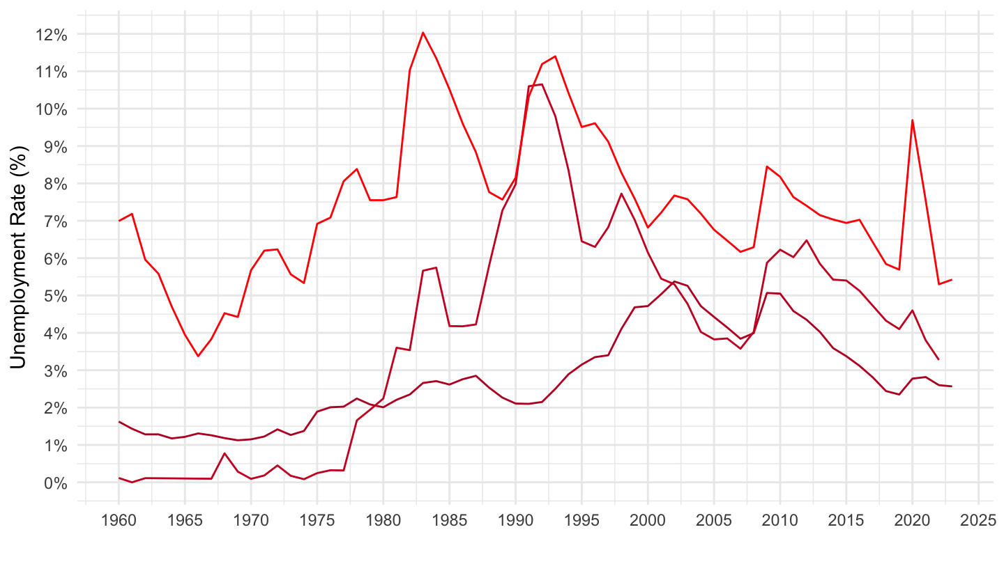
United States, Europe, France
Annual
Code
STLABOUR %>%
  # LRHUTTTT: Harmonised unemployment Rate (monthly), Total, All persons
  # ST: Level, rate or quantity series
  filter(SUBJECT == "LRHUTTTT",
         MEASURE == "ST",
         FREQUENCY == "A",
         LOCATION %in% c("USA", "EA20", "FRA")) %>%
  left_join(STLABOUR_var$LOCATION, by = "LOCATION") %>%
  frequency_to_date %>%
  mutate(Location = ifelse(LOCATION == "EA20", "Europe", Location)) %>%
  mutate(obsValue = obsValue/100) %>%
  left_join(colors, by = c("Location" = "country")) %>%
  ggplot() + geom_line(aes(x = date, y = obsValue, color = color)) + theme_minimal() +
  scale_color_identity() + add_3flags +
  scale_x_date(breaks = seq(1920, 2100, 5) %>% paste0("-01-01") %>% as.Date,
               labels = date_format("%Y")) +
  theme(legend.position = c(0.15, 0.9),
        legend.title = element_blank()) +
  scale_y_continuous(breaks = 0.01*seq(-7, 80, 1),
                     labels = scales::percent_format(accuracy = 1)) +
  ylab("Unemployment Rate (%)") + xlab("")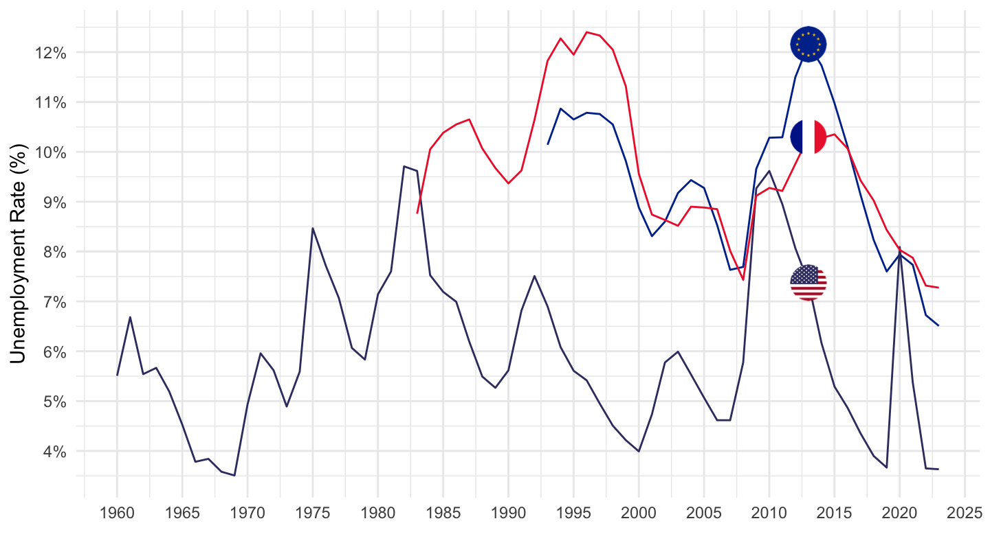
Quarterly
Code
STLABOUR %>%
  # LRHUTTTT: Harmonised unemployment Rate (monthly), Total, All persons
  # ST: Level, rate or quantity series
  filter(SUBJECT == "LRHUTTTT",
         MEASURE == "ST",
         FREQUENCY == "Q",
         LOCATION %in% c("USA", "EA20", "FRA")) %>%
  left_join(STLABOUR_var$LOCATION, by = "LOCATION") %>%
  frequency_to_date %>%
  mutate(Location = ifelse(LOCATION == "EA20", "Europe", Location)) %>%
  mutate(obsValue = obsValue/100) %>%
  left_join(colors, by = c("Location" = "country")) %>%
  ggplot() + geom_line(aes(x = date, y = obsValue, color = color)) + theme_minimal() +
  scale_color_identity() + add_3flags +
  scale_x_date(breaks = seq(1920, 2100, 5) %>% paste0("-01-01") %>% as.Date,
               labels = date_format("%Y")) +
  theme(legend.position = c(0.15, 0.9),
        legend.title = element_blank()) +
  scale_y_continuous(breaks = 0.01*seq(-7, 80, 1),
                     labels = scales::percent_format(accuracy = 1)) +
  ylab("Unemployment Rate (%)") + xlab("")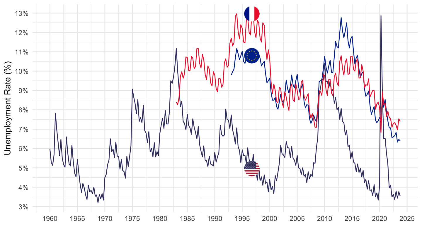
Monthly
All
Code
STLABOUR %>%
  # LRHUTTTT: Harmonised unemployment Rate (monthly), Total, All persons
  # ST: Level, rate or quantity series
  filter(SUBJECT == "LRHUTTTT",
         MEASURE == "ST",
         FREQUENCY == "M",
         LOCATION %in% c("USA", "EA20", "FRA")) %>%
  left_join(STLABOUR_var$LOCATION, by = "LOCATION") %>%
  frequency_to_date %>%
  mutate(Location = ifelse(LOCATION == "EA20", "Europe", Location)) %>%
  mutate(obsValue = obsValue/100) %>%
  left_join(colors, by = c("Location" = "country")) %>%
  ggplot() + geom_line(aes(x = date, y = obsValue, color = color)) + theme_minimal() +
  scale_color_identity() + add_3flags +
  scale_x_date(breaks = seq(1920, 2100, 5) %>% paste0("-01-01") %>% as.Date,
               labels = date_format("%Y")) +
  theme(legend.position = c(0.15, 0.9),
        legend.title = element_blank()) +
  scale_y_continuous(breaks = 0.01*seq(-7, 80, 1),
                     labels = scales::percent_format(accuracy = 1)) +
  ylab("Unemployment Rate (%)") + xlab("")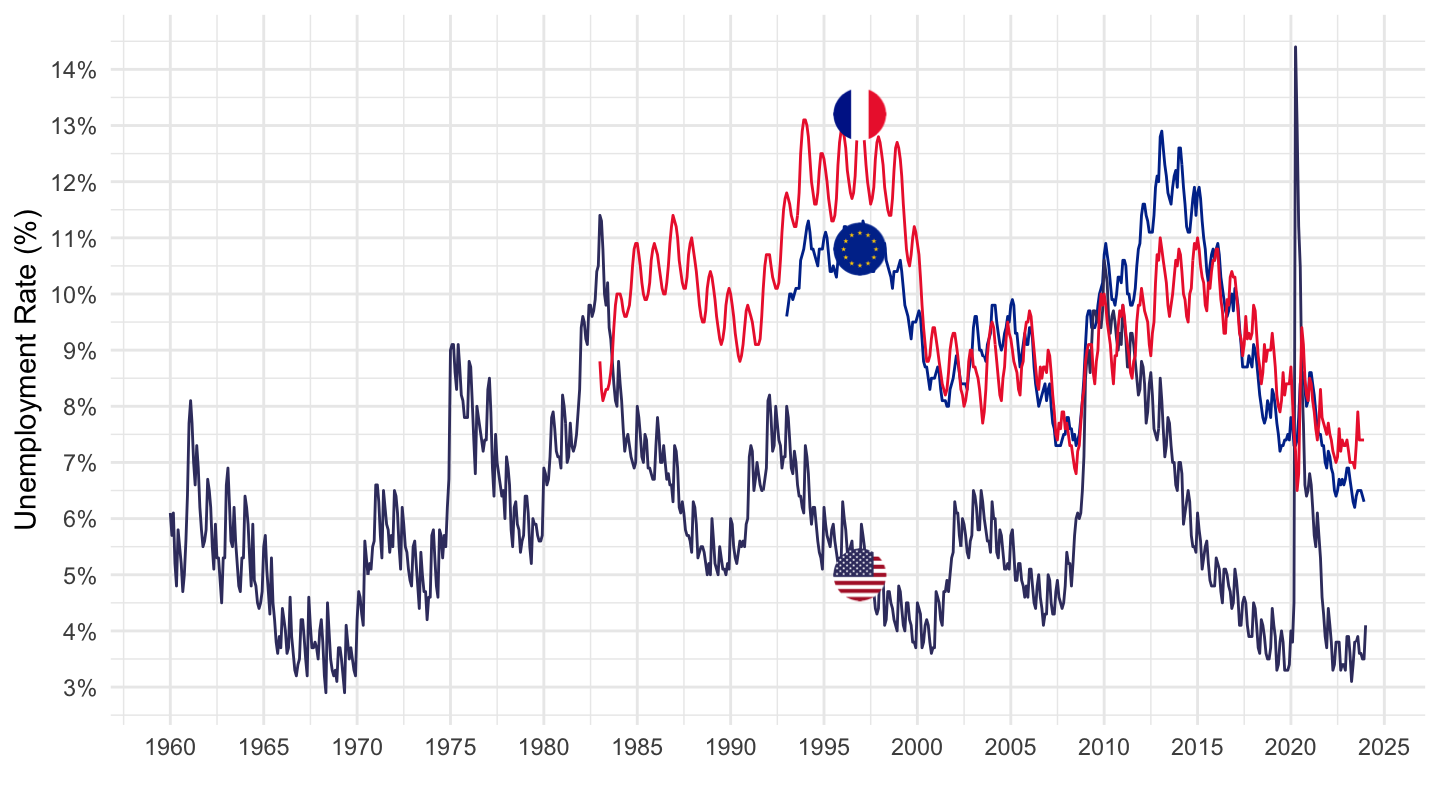
1990-
Code
STLABOUR %>%
  # LRHUTTTT: Harmonised unemployment Rate (monthly), Total, All persons
  # ST: Level, rate or quantity series
  filter(SUBJECT == "LRHUTTTT",
         MEASURE == "ST",
         FREQUENCY == "M",
         LOCATION %in% c("USA", "EA20", "FRA")) %>%
  left_join(STLABOUR_var$LOCATION, by = "LOCATION") %>%
  frequency_to_date %>%
  mutate(Location = ifelse(LOCATION == "EA20", "Europe", Location)) %>%
  mutate(obsValue = obsValue/100) %>%
  filter(date >= as.Date("1990-01-01")) %>%
  left_join(colors, by = c("Location" = "country")) %>%
  mutate(color = ifelse(LOCATION == "EA20", color2, color)) %>%
  ggplot() + geom_line(aes(x = date, y = obsValue, color = color)) + theme_minimal() +
  scale_color_identity() + add_3flags +
  scale_x_date(breaks = seq(1920, 2100, 5) %>% paste0("-01-01") %>% as.Date,
               labels = date_format("%Y")) +
  theme(legend.position = c(0.15, 0.9),
        legend.title = element_blank()) +
  scale_y_continuous(breaks = 0.01*seq(-7, 80, 1),
                     labels = scales::percent_format(accuracy = 1)) +
  ylab("Unemployment Rate (%)") + xlab("")
1999-
Code
plot <- STLABOUR %>%
  # LRHUTTTT: Harmonised unemployment Rate (monthly), Total, All persons
  # ST: Level, rate or quantity series
  filter(SUBJECT == "LRHUTTTT",
         MEASURE == "ST",
         FREQUENCY == "M",
         LOCATION %in% c("USA", "EA20")) %>%
  left_join(STLABOUR_var$LOCATION, by = "LOCATION") %>%
  frequency_to_date %>%
  mutate(Location = ifelse(LOCATION == "EA20", "Zone euro", "Etats-Unis")) %>%
  mutate(obsValue = obsValue/100) %>%
  filter(date >= as.Date("1999-01-01")) %>%
  ggplot() + geom_line(aes(x = date, y = obsValue, color = Location)) +
  scale_color_manual(values = c("#B22234", "#003399")) +
  geom_rect(data = nber_recessions %>%
              filter(Peak > as.Date("1999-01-01")),
            aes(xmin = Peak, xmax = Trough, ymin = 0, ymax = +Inf),
            fill = '#B22234', alpha = 0.1)  +
  geom_rect(data = cepr_recessions %>%
              filter(Peak > as.Date("1999-01-01")),
            aes(xmin = Peak, xmax = Trough, ymin = 0, ymax = +Inf),
            fill = '#003399', alpha = 0.1) +
  theme_minimal() +
  scale_x_date(breaks = c(seq(1999, 2100, 5), seq(2002, 2100, 5)) %>% paste0("-01-01") %>% as.Date,
               labels = date_format("%Y")) +
  theme(legend.position = c(0.15, 0.9),
        legend.title = element_blank()) +
  scale_y_continuous(breaks = 0.01*seq(-7, 80, 1),
                     labels = scales::percent_format(accuracy = 1)) +
  ylab("Taux de chômage (%)") + xlab("")

plot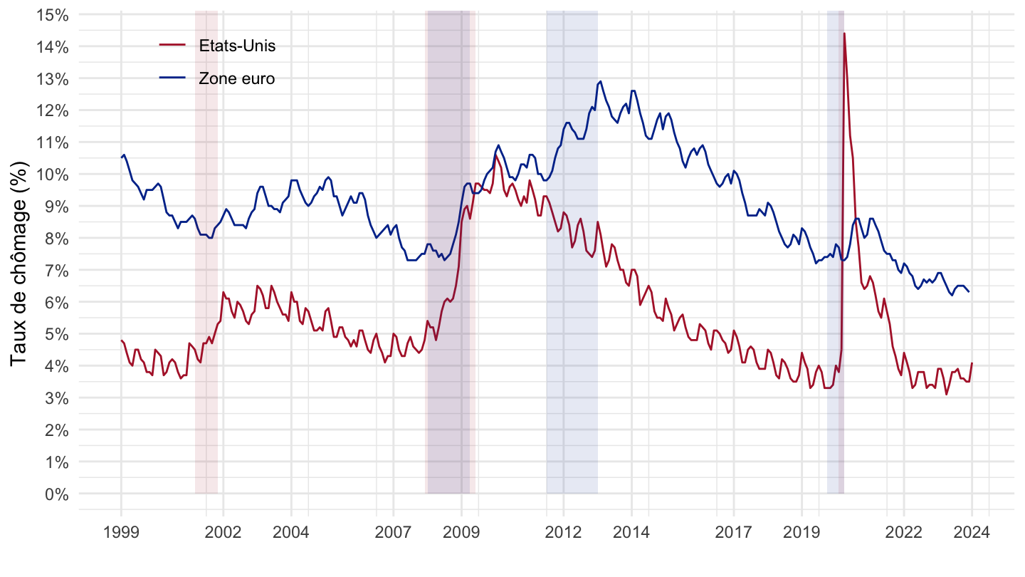
Code
save(plot, file = "STLABOUR_files/figure-html/LRHUTTTT-M-USA-EA20-1999-1.RData")2005-
Code
STLABOUR %>%
  # LRHUTTTT: Harmonised unemployment Rate (monthly), Total, All persons
  # ST: Level, rate or quantity series
  filter(SUBJECT == "LRHUTTTT",
         MEASURE == "ST",
         FREQUENCY == "M",
         LOCATION %in% c("USA", "EA20", "FRA")) %>%
  left_join(STLABOUR_var$LOCATION, by = "LOCATION") %>%
  frequency_to_date %>%
  mutate(Location = ifelse(LOCATION == "EA20", "Europe", Location)) %>%
  mutate(obsValue = obsValue/100) %>%
  filter(date >= as.Date("2005-01-01")) %>%
  left_join(colors, by = c("Location" = "country")) %>%
  mutate(color = ifelse(LOCATION == "EA20", color2, color)) %>%
  ggplot() + geom_line(aes(x = date, y = obsValue, color = color)) + theme_minimal() +
  scale_color_identity() + add_3flags +
  scale_x_date(breaks = seq(1920, 2100, 2) %>% paste0("-01-01") %>% as.Date,
               labels = date_format("%Y")) +
  theme(legend.position = c(0.15, 0.9),
        legend.title = element_blank()) +
  scale_y_continuous(breaks = 0.01*seq(-7, 80, 1),
                     labels = scales::percent_format(accuracy = 1)) +
  ylab("Unemployment Rate (%)") + xlab("")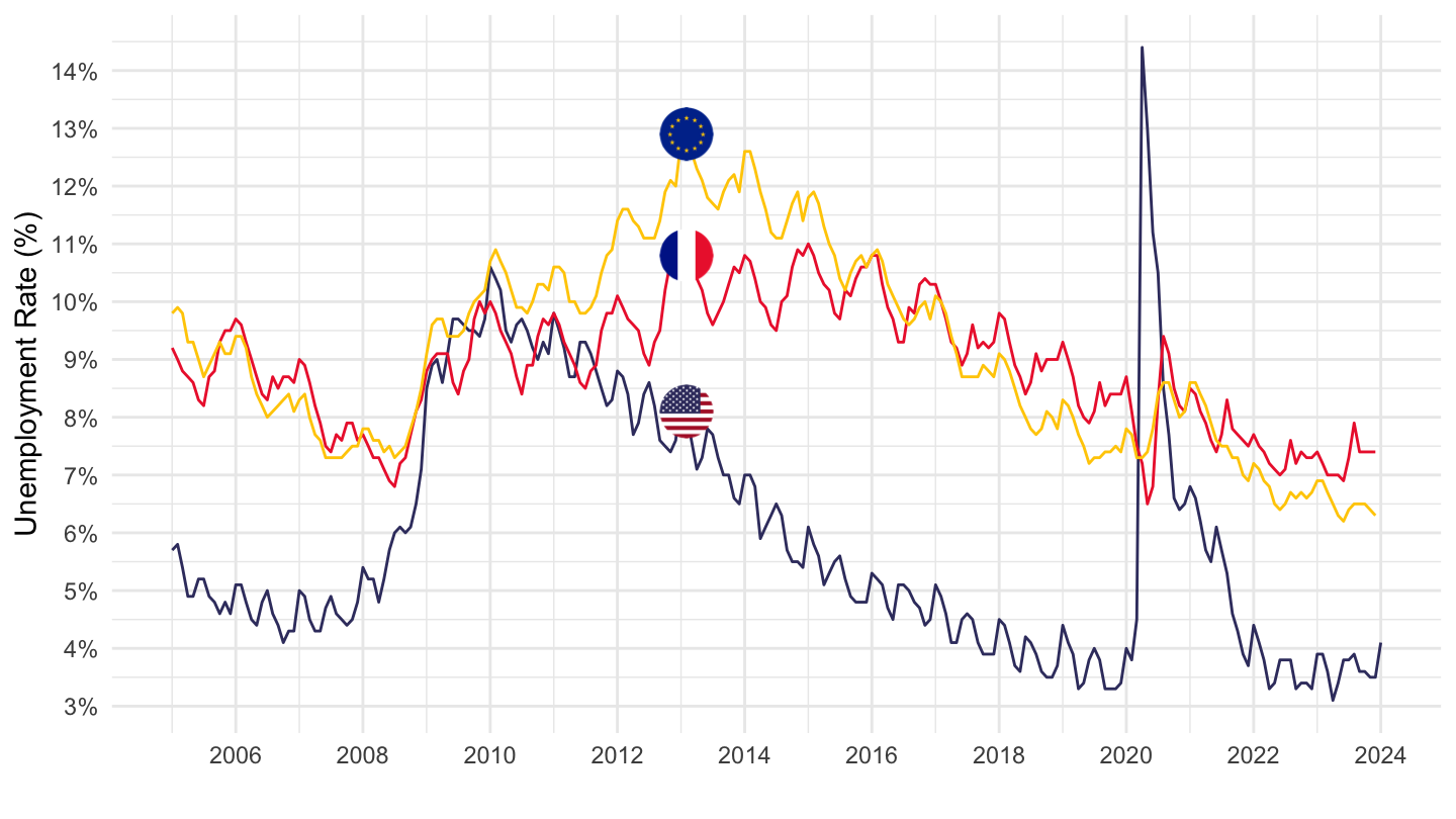
United States, Australia, Belgium
Annual
Code
STLABOUR %>%
  # LRHUTTTT: Harmonised unemployment Rate (monthly), Total, All persons
  # ST: Level, rate or quantity series
  filter(SUBJECT == "LRHUTTTT",
         MEASURE == "ST",
         FREQUENCY == "A",
         LOCATION %in% c("USA", "AUS", "BEL")) %>%
  left_join(STLABOUR_var$LOCATION, by = "LOCATION") %>%
  frequency_to_date %>%
  mutate(obsValue = obsValue/100) %>%
  left_join(colors, by = c("Location" = "country")) %>%
  ggplot() + geom_line(aes(x = date, y = obsValue, color = color)) + theme_minimal() +
  scale_color_identity() + add_3flags +
  scale_x_date(breaks = seq(1920, 2100, 5) %>% paste0("-01-01") %>% as.Date,
               labels = date_format("%Y")) +
  theme(legend.position = c(0.15, 0.9),
        legend.title = element_blank()) +
  scale_y_continuous(breaks = 0.01*seq(-7, 80, 1),
                     labels = scales::percent_format(accuracy = 1)) +
  ylab("Unemployment Rate (%)") + xlab("")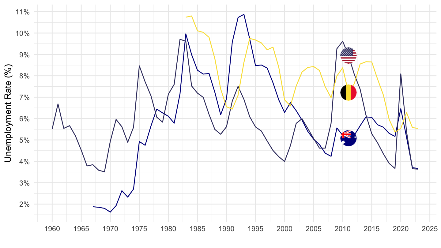
Quarterly
Code
STLABOUR %>%
  # LRHUTTTT: Harmonised unemployment Rate (monthly), Total, All persons
  # ST: Level, rate or quantity series
  filter(SUBJECT == "LRHUTTTT",
         MEASURE == "ST",
         FREQUENCY == "Q",
         LOCATION %in% c("USA", "AUS", "BEL")) %>%
  left_join(STLABOUR_var$LOCATION, by = "LOCATION") %>%
  frequency_to_date %>%
  mutate(obsValue = obsValue/100) %>%
  left_join(colors, by = c("Location" = "country")) %>%
  ggplot() + geom_line(aes(x = date, y = obsValue, color = color)) + theme_minimal() +
  scale_color_identity() + add_3flags +
  scale_x_date(breaks = seq(1920, 2100, 5) %>% paste0("-01-01") %>% as.Date,
               labels = date_format("%Y")) +
  theme(legend.position = c(0.15, 0.9),
        legend.title = element_blank()) +
  scale_y_continuous(breaks = 0.01*seq(-7, 80, 1),
                     labels = scales::percent_format(accuracy = 1)) +
  ylab("Unemployment Rate (%)") + xlab("")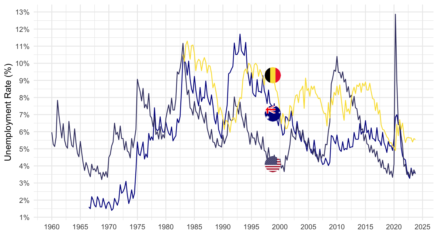
Monthly
Code
STLABOUR %>%
  # LRHUTTTT: Harmonised unemployment Rate (monthly), Total, All persons
  # ST: Level, rate or quantity series
  filter(SUBJECT == "LRHUTTTT",
         MEASURE == "ST",
         FREQUENCY == "M",
         LOCATION %in% c("USA", "AUS", "BEL")) %>%
  left_join(STLABOUR_var$LOCATION, by = "LOCATION") %>%
  frequency_to_date %>%
  mutate(obsValue = obsValue/100) %>%
  left_join(colors, by = c("Location" = "country")) %>%
  ggplot() + geom_line(aes(x = date, y = obsValue, color = color)) + theme_minimal() +
  scale_color_identity() + add_3flags +
  scale_x_date(breaks = seq(1920, 2100, 5) %>% paste0("-01-01") %>% as.Date,
               labels = date_format("%Y")) +
  theme(legend.position = c(0.15, 0.9),
        legend.title = element_blank()) +
  scale_y_continuous(breaks = 0.01*seq(-7, 80, 1),
                     labels = scales::percent_format(accuracy = 1)) +
  ylab("Unemployment Rate (%)") + xlab("")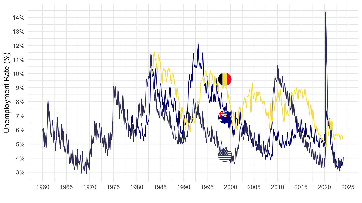
Germany, France, United States
All
Code
STLABOUR %>%
  # LRHUTTTT: Harmonised unemployment Rate (monthly), Total, All persons
  # ST: Level, rate or quantity series
  filter(SUBJECT == "LRHUTTTT",
         MEASURE == "ST",
         FREQUENCY == "Q",
         LOCATION %in% c("DEU", "FRA", "USA")) %>%
  left_join(STLABOUR_var$LOCATION, by = "LOCATION") %>%
  quarter_to_date %>%
  mutate(obsValue = obsValue/100) %>%
  ggplot() + geom_line(aes(x = date, y = obsValue, color = Location)) + theme_minimal() +
  add_3flags +
  scale_color_manual(values = c("#002395", "#000000", "#B22234")) +
  scale_x_date(breaks = seq(1920, 2100, 5) %>% paste0("-01-01") %>% as.Date,
               labels = date_format("%Y")) +
  theme(legend.position = c(0.15, 0.9),
        legend.title = element_blank()) +
  scale_y_continuous(breaks = 0.01*seq(-7, 80, 1),
                     labels = scales::percent_format(accuracy = 1)) +
  ylab("Unemployment Rate (%)") + xlab("")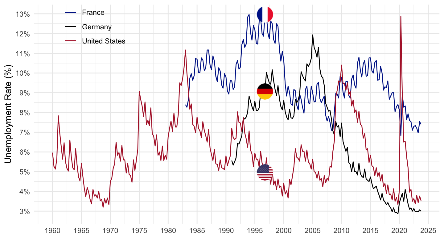
1990-
Code
STLABOUR %>%
  # LRHUTTTT: Harmonised unemployment Rate (monthly), Total, All persons
  # ST: Level, rate or quantity series
  filter(SUBJECT == "LRHUTTTT",
         MEASURE == "ST",
         FREQUENCY == "Q",
         LOCATION %in% c("DEU", "FRA", "USA")) %>%
  left_join(STLABOUR_var$LOCATION, by = "LOCATION") %>%
  quarter_to_date %>%
  mutate(obsValue = obsValue/100) %>%
  filter(date >= as.Date("1990-01-01")) %>%
  ggplot() + geom_line(aes(x = date, y = obsValue, color = Location)) + theme_minimal() +
  add_3flags +
  scale_color_manual(values = c("#002395", "#000000", "#B22234")) +
  scale_x_date(breaks = seq(1920, 2100, 5) %>% paste0("-01-01") %>% as.Date,
               labels = date_format("%Y")) +
  theme(legend.position = c(0.15, 0.9),
        legend.title = element_blank()) +
  scale_y_continuous(breaks = 0.01*seq(-7, 80, 1),
                     labels = scales::percent_format(accuracy = 1)) +
  ylab("Unemployment Rate (%)") + xlab("")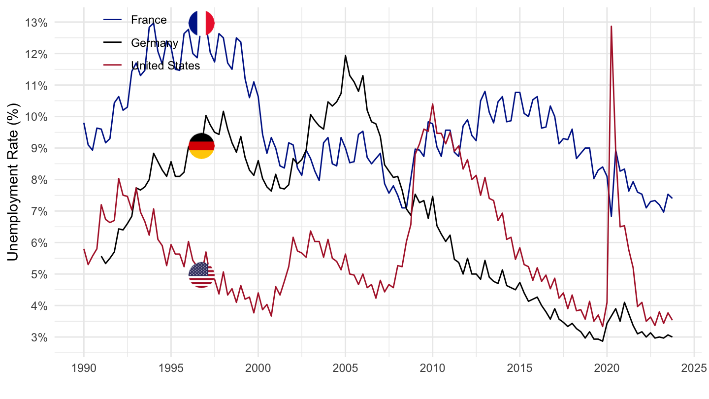
Germany, United Kingdom, United States
Code
STLABOUR %>%
  # LRHUTTTT: Harmonised unemployment Rate (monthly), Total, All persons
  # ST: Level, rate or quantity series
  filter(SUBJECT == "LRHUTTTT",
         MEASURE == "ST",
         FREQUENCY == "Q",
         LOCATION %in% c("DEU", "GBR", "USA")) %>%
  left_join(STLABOUR_var$LOCATION, by = "LOCATION") %>%
  quarter_to_date %>%
  ggplot() + geom_line(aes(x = date, y = obsValue/100, color = Location)) + theme_minimal() +
  geom_image(data = . %>%
               filter(date == as.Date("1998-01-01")) %>%
               mutate(image = paste0("../../icon/flag/round/", str_to_lower(gsub(" ", "-", Location)), ".png")),
             aes(x = date, y = obsValue/100, image = image), asp = 1.5) +
  scale_color_manual(values = c("#000000", "#CF142B", "#3C3B6E")) +
  scale_x_date(breaks = seq(1920, 2100, 5) %>% paste0("-01-01") %>% as.Date,
               labels = date_format("%Y")) +
  theme(legend.position = c(0.15, 0.9),
        legend.title = element_blank()) +
  scale_y_continuous(breaks = 0.01*seq(-7, 80, 1),
                     labels = scales::percent_format(accuracy = 1)) +
  ylab("Unemployment Rate (%)") + xlab("")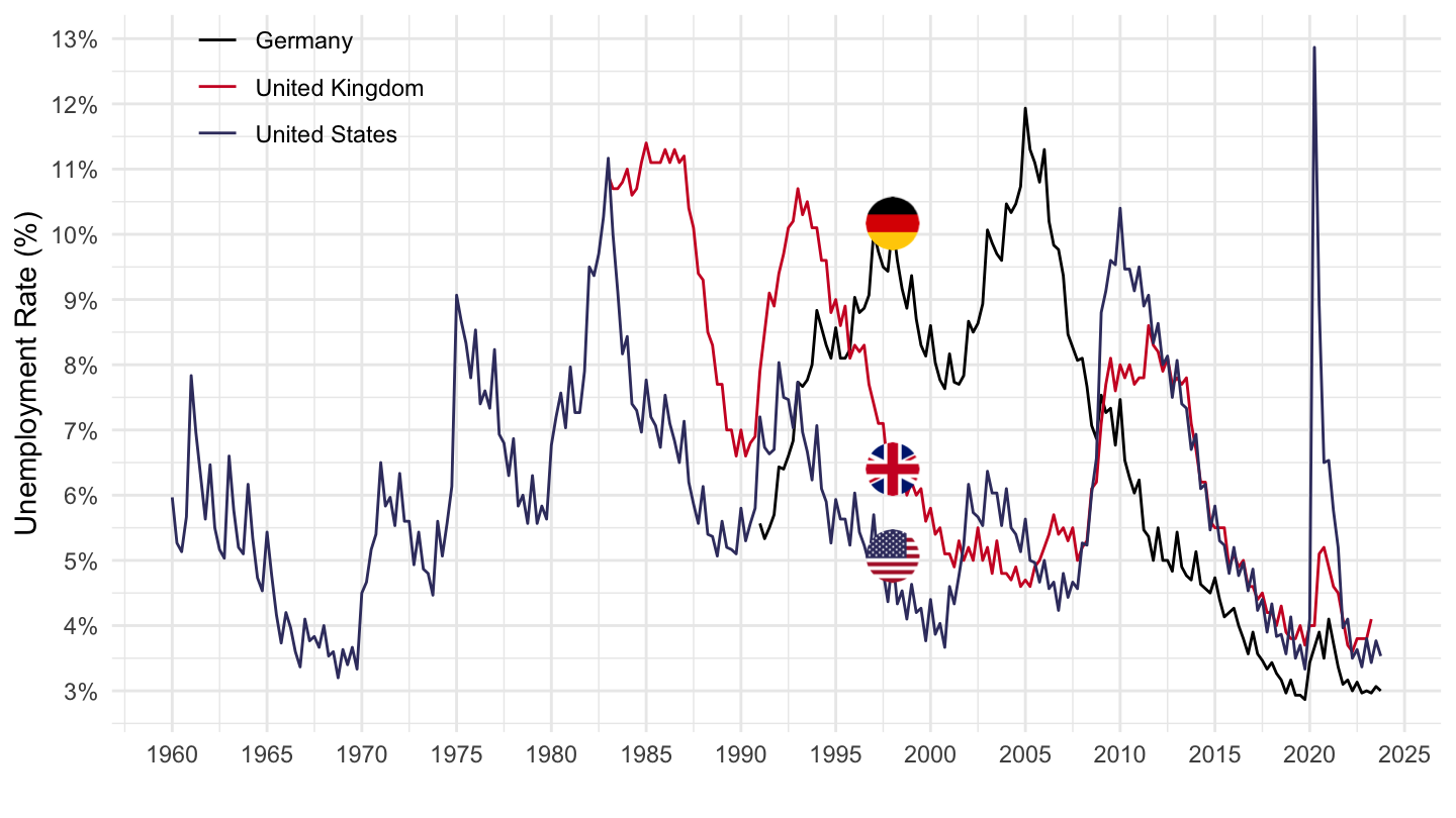
Germany, France, Italy
Code
STLABOUR %>%
  # LRHUTTTT: Harmonised unemployment Rate (monthly), Total, All persons
  # ST: Level, rate or quantity series
  filter(SUBJECT == "LRHUTTTT",
         MEASURE == "ST",
         FREQUENCY == "Q",
         LOCATION %in% c("DEU", "FRA", "ITA")) %>%
  left_join(STLABOUR_var$LOCATION, by = "LOCATION") %>%
  quarter_to_date %>%
  ggplot() + geom_line(aes(x = date, y = obsValue/100, color = Location)) + theme_minimal() +
  geom_image(data = . %>%
               filter(date == as.Date("2015-01-01")) %>%
               mutate(image = paste0("../../icon/flag/round/", str_to_lower(gsub(" ", "-", Location)), ".png")),
             aes(x = date, y = obsValue/100, image = image), asp = 1.5) +
  scale_color_manual(values = c( "#0055a4", "#000000", "#008c45")) +
  scale_x_date(breaks = seq(1920, 2100, 5) %>% paste0("-01-01") %>% as.Date,
               labels = date_format("%Y")) +
  theme(legend.position = c(0.15, 0.9),
        legend.title = element_blank()) +
  scale_y_continuous(breaks = 0.01*seq(-7, 80, 1),
                     labels = scales::percent_format(accuracy = 1)) +
  ylab("Unemployment Rate (%)") + xlab("")