Unemployment by sex and age – monthly data
Data - Eurostat
Info
Last observation: Monthly: 2026M06 (N = 162)
First observation: Monthly: 1983M01 (N = 493)
Last data update: 23 jul 2026, 22:08. Last compile: 24 jul 2026, 04:08
Structure
Young
France, Germany, Spain, Italy, Eurozone
All
Code
une_rt_m %>%
  filter(geo %in% c("FR", "DE", "IT", "ES", "EA21"),
         age == "Y_LT25",
         sex == "T",
         unit == "PC_ACT",
         s_adj == "SA") %>%
  month_to_date %>%

  mutate(values = values/100,
         Geo = ifelse(geo == "EA21", "Europe", Geo)) %>%
  left_join(colors, by = c("Geo" = "country")) %>%
  ggplot + geom_line(aes(x = date, y = values, color = color)) +
  theme_minimal() + scale_color_identity() + add_5flags +
  scale_x_date(breaks = as.Date(paste0(seq(1960, 2100, 5), "-01-01")),
               labels = date_format("%Y")) +
  xlab("") + ylab("Unemployment, Percentage of active population") +
  scale_y_continuous(breaks = 0.01*seq(0, 200, 2),
                     labels = scales::percent_format(accuracy = 1))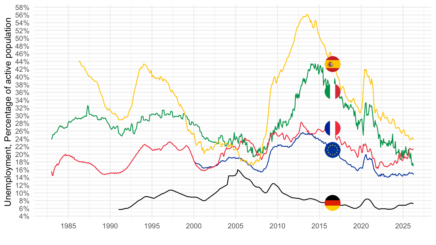
France, Germany, Netherlands, Sweden
All
Code
une_rt_m %>%
  filter(geo %in% c("FR", "DE", "NL", "SE", "EA21"),
         age == "Y_LT25",
         sex == "T",
         unit == "PC_ACT",
         s_adj == "SA") %>%
  month_to_date %>%

  mutate(values = values/100,
         Geo = ifelse(geo == "EA21", "Europe", Geo)) %>%
  left_join(colors, by = c("Geo" = "country")) %>%
  ggplot + geom_line(aes(x = date, y = values, color = color)) +
  theme_minimal() + scale_color_identity() + add_5flags +
  scale_x_date(breaks = as.Date(paste0(seq(1960, 2100, 5), "-01-01")),
               labels = date_format("%Y")) +
  xlab("") + ylab("Unemployment, Percentage of active population") +
  scale_y_continuous(breaks = 0.01*seq(0, 200, 2),
                     labels = scales::percent_format(accuracy = 1))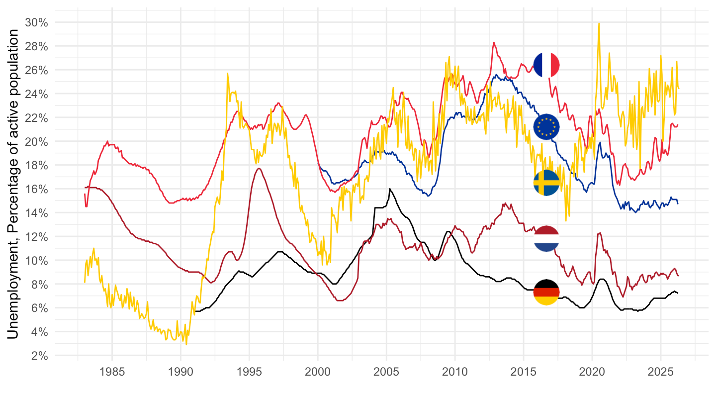
All age, All sex
France, Germany, Spain, Italy, Netherlands, Portugal, EA
All
Code
une_rt_m %>%
  filter(geo %in% c("FR", "DE", "IT", "ES", "NL", "PT", "EA21"),
         age == "TOTAL",
         sex == "T",
         unit == "PC_ACT",
         s_adj == "SA") %>%
  month_to_date %>%

  mutate(values = values/100,
         Geo = ifelse(geo == "EA21", "Europe", Geo)) %>%
  left_join(colors, by = c("Geo" = "country")) %>%
  ggplot + geom_line(aes(x = date, y = values, color = color)) +
  theme_minimal() + scale_color_identity() + add_7flags +
  scale_x_date(breaks = as.Date(paste0(seq(1960, 2100, 5), "-01-01")),
               labels = date_format("%Y")) +
  xlab("") + ylab("Unemployment, Percentage of active population") +
  scale_y_continuous(breaks = 0.01*seq(0, 200, 2),
                     labels = scales::percent_format(accuracy = 1))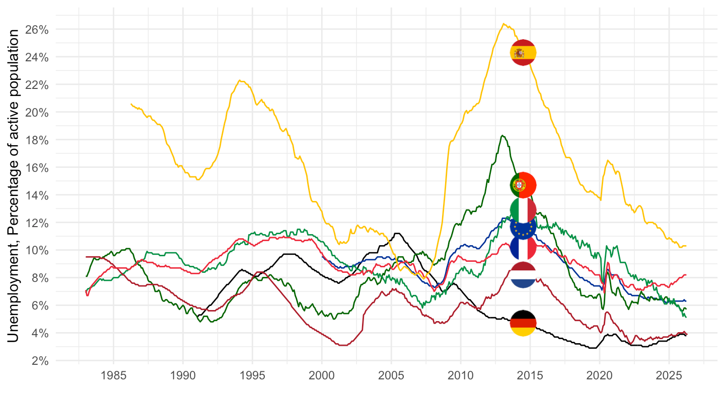
2002-
Code
une_rt_m %>%
  filter(geo %in% c("FR", "DE", "IT", "ES", "NL", "PT", "EA21"),
         age == "TOTAL",
         sex == "T",
         unit == "PC_ACT",
         s_adj == "SA") %>%
  month_to_date %>%

  mutate(values = values/100,
         Geo = ifelse(geo == "EA21", "Europe", Geo)) %>%
  left_join(colors, by = c("Geo" = "country")) %>%
  filter(date >= as.Date("2002-01-01")) %>%
  ggplot + geom_line(aes(x = date, y = values, color = color)) +
  theme_minimal() +
  theme(axis.text.x = element_text(angle = 45, vjust = 1, hjust = 1))+
  scale_color_identity() + add_7flags +
  scale_x_date(breaks = as.Date(paste0(seq(1960, 2100, 1), "-01-01")),
               labels = date_format("%Y")) +
  xlab("") + ylab("Unemployment, Percentage of active population") +
  scale_y_continuous(breaks = 0.01*seq(0, 200, 2),
                     labels = scales::percent_format(accuracy = 1)) +
  geom_text_repel(data = . %>%
                    filter(date == max(date)), aes(x = date, y = values, label = percent(values)))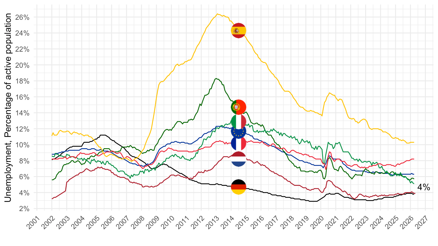
2002-
Code
une_rt_m %>%
  filter(geo %in% c("FR", "DE", "IT", "NL", "PT", "EA21"),
         age == "TOTAL",
         sex == "T",
         unit == "PC_ACT",
         s_adj == "SA") %>%
  month_to_date %>%

  mutate(values = values/100,
         Geo = ifelse(geo == "EA21", "Europe", Geo)) %>%
  left_join(colors, by = c("Geo" = "country")) %>%
  filter(date >= as.Date("2002-01-01")) %>%
  ggplot + geom_line(aes(x = date, y = values, color = color)) +
  theme_minimal() +
  theme(axis.text.x = element_text(angle = 45, vjust = 1, hjust = 1))+
  scale_color_identity() + add_6flags +
  scale_x_date(breaks = as.Date(paste0(seq(1960, 2100, 1), "-01-01")),
               labels = date_format("%Y")) +
  xlab("") + ylab("Unemployment, Percentage of active population") +
  scale_y_continuous(breaks = 0.01*seq(0, 200, 2),
                     labels = scales::percent_format(accuracy = 1)) +
  geom_label_repel(data = . %>%
                    filter(date == max(date)), aes(x = date, y = values, label = percent(values, acc = .1), color = color))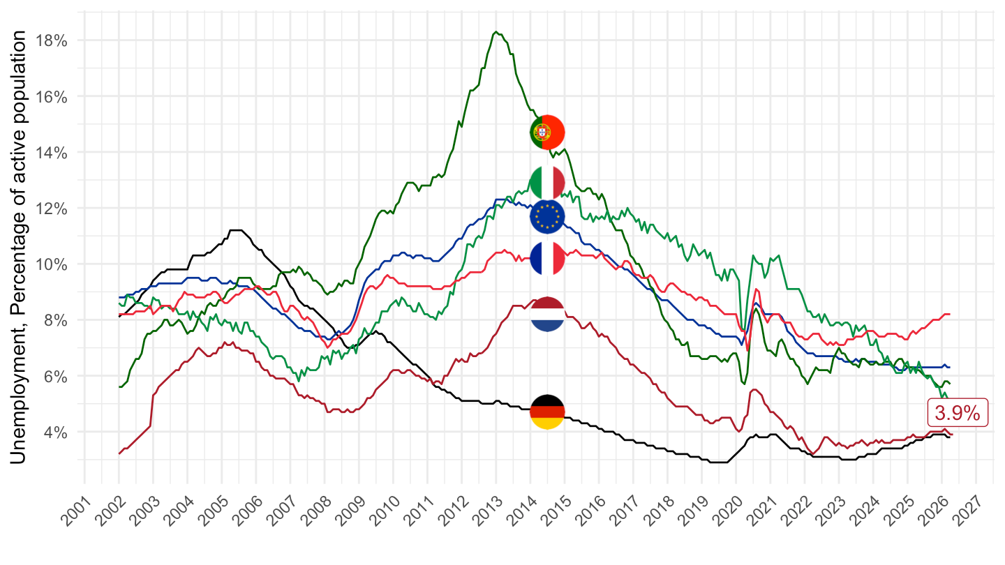
2007-
Code
une_rt_m %>%
  filter(geo %in% c("FR", "DE", "IT", "NL", "PT", "EA21"),
         age == "TOTAL",
         sex == "T",
         unit == "PC_ACT",
         s_adj == "SA") %>%
  month_to_date %>%

  mutate(values = values/100,
         Geo = ifelse(geo == "EA21", "Europe", Geo)) %>%
  left_join(colors, by = c("Geo" = "country")) %>%
  filter(date >= as.Date("2007-01-01")) %>%
  ggplot + geom_line(aes(x = date, y = values, color = color)) +
  theme_minimal() +
  theme(axis.text.x = element_text(angle = 45, vjust = 1, hjust = 1))+
  scale_color_identity() + add_6flags +
  scale_x_date(breaks = as.Date(paste0(seq(1960, 2100, 1), "-01-01")),
               labels = date_format("%Y")) +
  xlab("") + ylab("Taux de chômage (% de la population active)") +
  scale_y_continuous(breaks = 0.01*seq(0, 200, 1),
                     labels = scales::percent_format(accuracy = 1),
                     limits = c(0, 0.19)) +
  geom_text_repel(data = . %>%
                    filter(date == max(date)), aes(x = date, y = values, label = percent(values, acc = .1), color = color))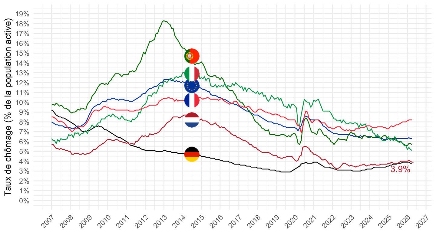
France, Germany, Spain, Italy, Eurozone
All
All age
Code
une_rt_m %>%
  filter(geo %in% c("FR", "DE", "IT", "ES", "EA21"),
         age == "TOTAL",
         sex == "T",
         unit == "PC_ACT",
         s_adj == "SA") %>%
  month_to_date %>%

  mutate(values = values/100,
         Geo = ifelse(geo == "EA21", "Europe", Geo)) %>%
  left_join(colors, by = c("Geo" = "country")) %>%
  ggplot + geom_line(aes(x = date, y = values, color = color)) +
  theme_minimal() + scale_color_identity() + add_5flags +
  scale_x_date(breaks = as.Date(paste0(seq(1960, 2100, 5), "-01-01")),
               labels = date_format("%Y")) +
  xlab("") + ylab("Unemployment, Percentage of active population") +
  scale_y_continuous(breaks = 0.01*seq(0, 200, 2),
                     labels = scales::percent_format(accuracy = 1))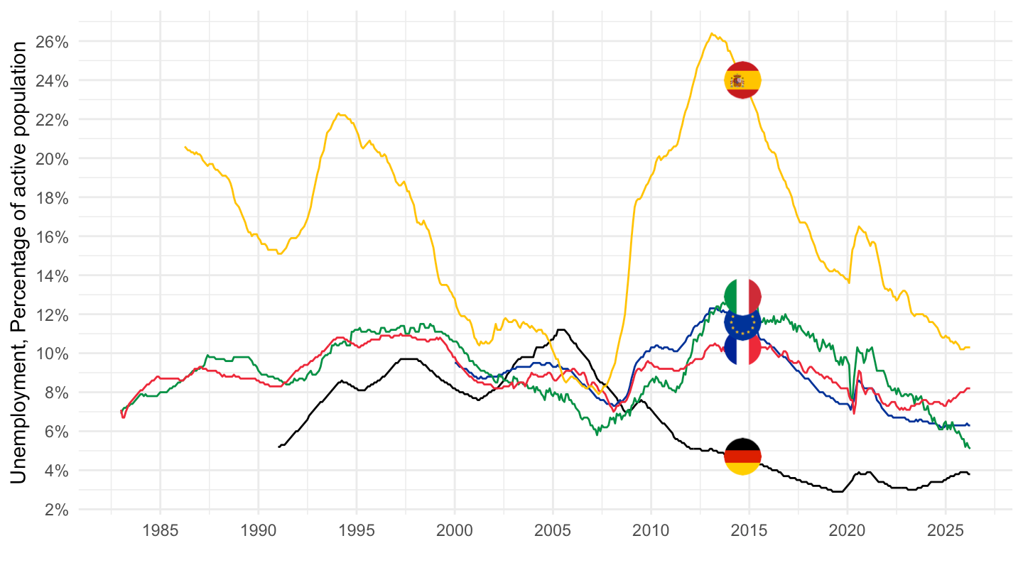
Youth
Code
une_rt_m %>%
  filter(geo %in% c("FR", "DE", "IT", "ES", "EA21"),
         age == "Y_LT25",
         sex == "T",
         unit == "PC_ACT",
         s_adj == "SA") %>%
  month_to_date %>%

  mutate(values = values/100,
         Geo = ifelse(geo == "EA21", "Europe", Geo)) %>%
  left_join(colors, by = c("Geo" = "country")) %>%
  ggplot + geom_line(aes(x = date, y = values, color = color)) +
  theme_minimal() + scale_color_identity() + add_5flags +
  scale_x_date(breaks = as.Date(paste0(seq(1960, 2100, 5), "-01-01")),
               labels = date_format("%Y")) +
  xlab("") + ylab("Younth Unemployment, % of active population") +
  scale_y_continuous(breaks = 0.01*seq(0, 200, 5),
                     labels = scales::percent_format(accuracy = 1))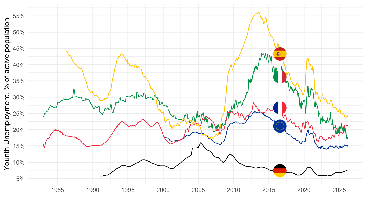
2010-
Code
une_rt_m %>%
  filter(geo %in% c("FR", "DE", "IT", "ES", "EA21"),
         age == "TOTAL",
         sex == "T",
         unit == "PC_ACT",
         s_adj == "SA") %>%
  month_to_date %>%

  left_join(colors, by = c("Geo" = "country")) %>%
  mutate(values = values/100,
         Geo = ifelse(geo == "EA21", "Europe", Geo)) %>%
  filter(date >= as.Date("2010-01-01")) %>%
  ggplot + geom_line(aes(x = date, y = values, color = color)) +
  theme_minimal() + scale_color_identity() + add_5flags +
  scale_x_date(breaks = as.Date(paste0(seq(1960, 2100, 1), "-01-01")),
               labels = date_format("%Y")) +
  xlab("") + ylab("Unemployment, Percentage of active population") +
  scale_y_continuous(breaks = 0.01*seq(0, 200, 2),
                     labels = scales::percent_format(accuracy = 1))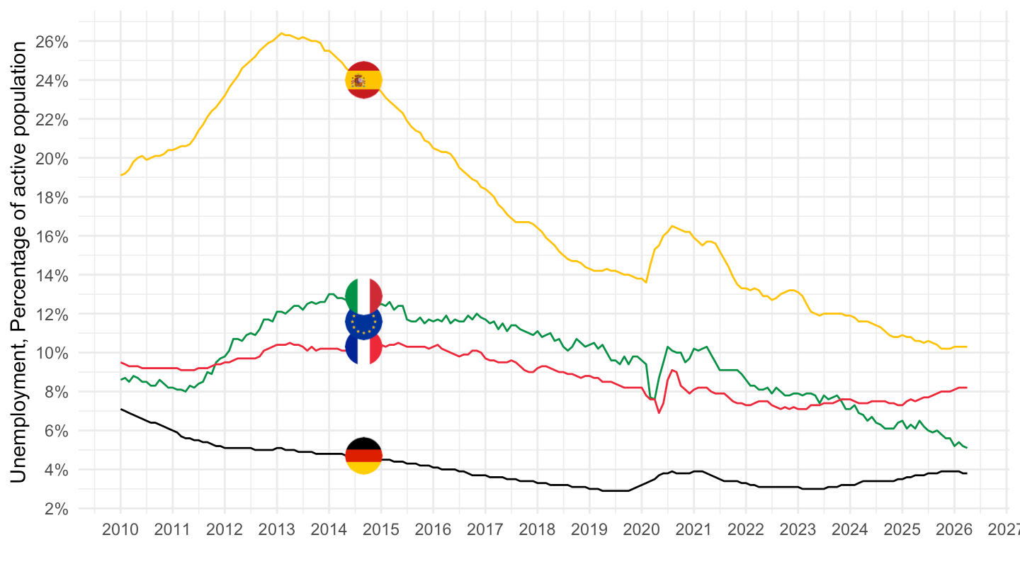
Youth
Code
une_rt_m %>%
  filter(geo %in% c("FR", "DE", "IT", "ES", "EA21"),
         age == "Y_LT25",
         sex == "T",
         unit == "PC_ACT",
         s_adj == "SA") %>%
  month_to_date %>%

  mutate(values = values/100,
         Geo = ifelse(geo == "EA21", "Europe", Geo)) %>%
  left_join(colors, by = c("Geo" = "country")) %>%
  filter(date >= as.Date("2010-01-01")) %>%
  ggplot + geom_line(aes(x = date, y = values, color = color)) +
  theme_minimal() + scale_color_identity() + add_5flags +
  scale_x_date(breaks = as.Date(paste0(seq(1960, 2100, 2), "-01-01")),
               labels = date_format("%Y")) +
  xlab("") + ylab("Younth Unemployment, % of active population") +
  scale_y_continuous(breaks = 0.01*seq(0, 200, 5),
                     labels = scales::percent_format(accuracy = 1))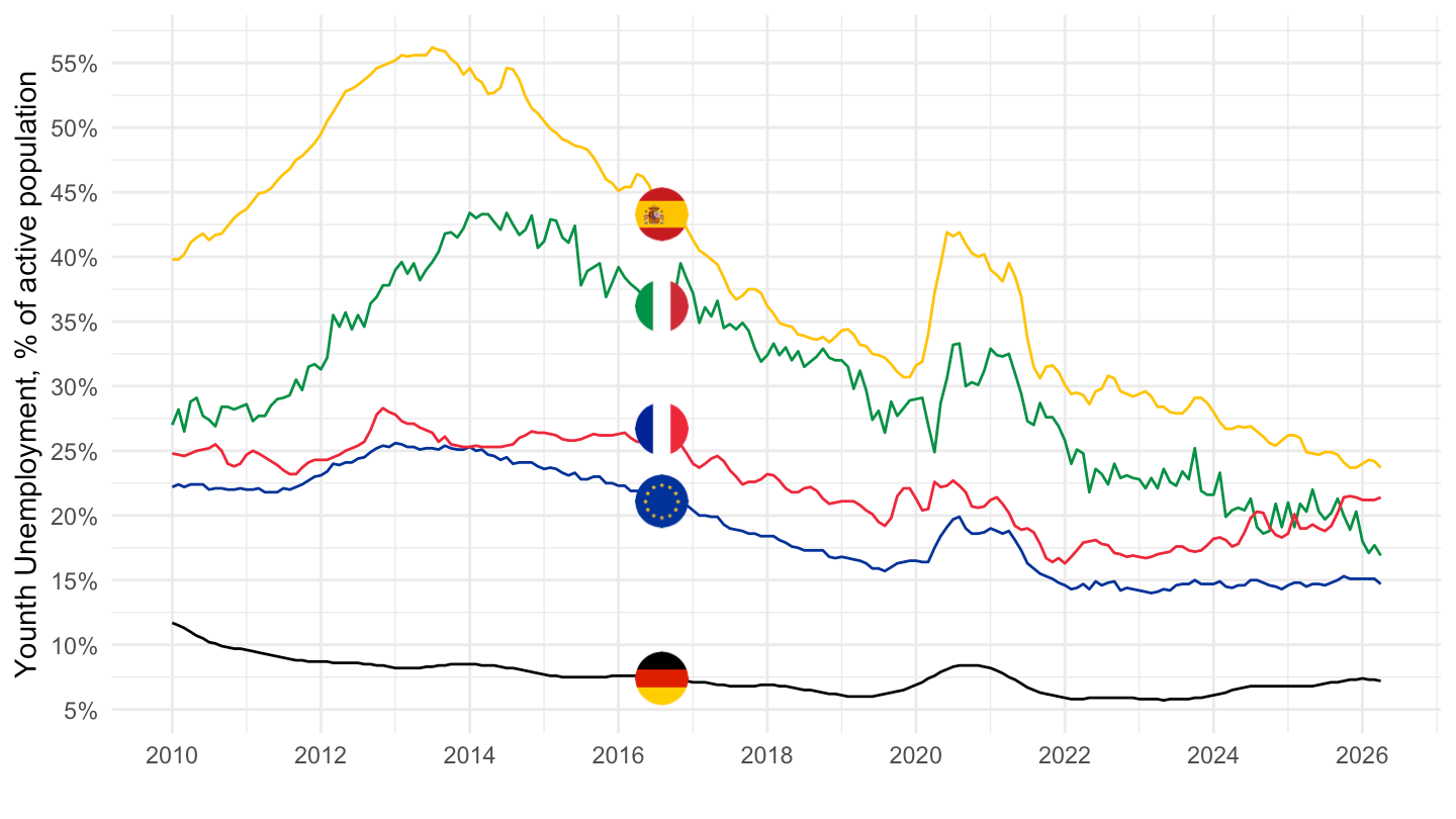
2014-
Code
une_rt_m %>%
  filter(geo %in% c("FR", "DE", "IT", "ES", "EA21"),
         age == "TOTAL",
         sex == "T",
         unit == "PC_ACT",
         s_adj == "SA") %>%
  month_to_date %>%

  left_join(colors, by = c("Geo" = "country")) %>%
  mutate(values = values/100,
         Geo = ifelse(geo == "EA21", "Europe", Geo)) %>%
  filter(date >= as.Date("2014-01-01")) %>%
  ggplot + geom_line(aes(x = date, y = values, color = color)) +
  theme_minimal() + scale_color_identity() + add_5flags +
  scale_x_date(breaks = as.Date(paste0(seq(1960, 2100, 1), "-01-01")),
               labels = date_format("%Y")) +
  xlab("") + ylab("Unemployment, Percentage of active population") +
  scale_y_continuous(breaks = 0.01*seq(0, 200, 2),
                     labels = scales::percent_format(accuracy = 1))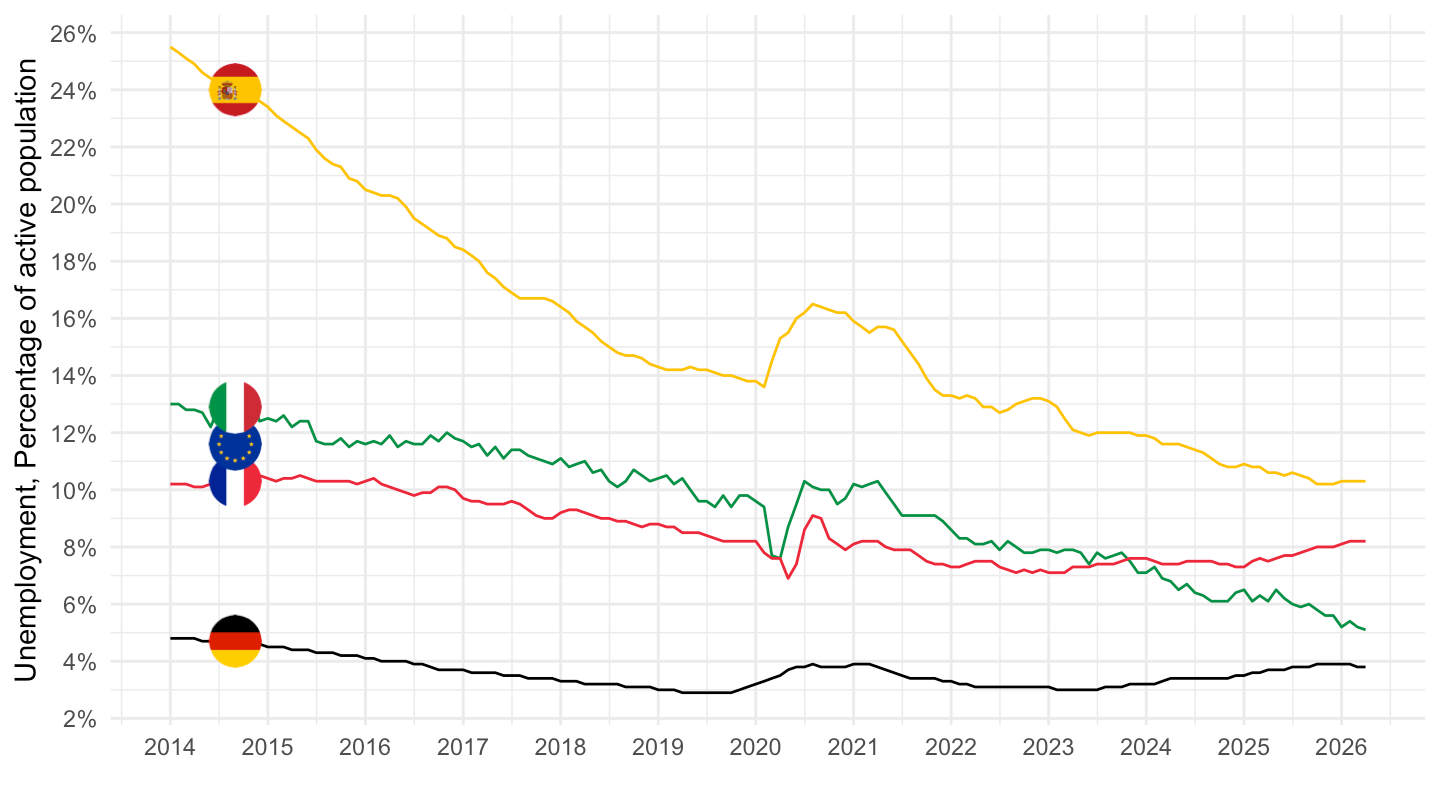
France, Germany, Spain, Italy, Netherlands, Portugal
All
Code
une_rt_m %>%
  filter(geo %in% c("FR", "DE", "IT", "ES", "NL", "PT"),
         age == "TOTAL",
         sex == "T",
         unit == "PC_ACT",
         s_adj == "SA") %>%
  month_to_date %>%

  left_join(colors, by = c("Geo" = "country")) %>%
  mutate(values = values/100) %>%
  ggplot + geom_line(aes(x = date, y = values, color = color)) +
  theme_minimal() + scale_color_identity() + add_6flags +
  scale_x_date(breaks = as.Date(paste0(seq(1960, 2100, 5), "-01-01")),
               labels = date_format("%Y")) +
  xlab("") + ylab("Unemployment, Percentage of active population") +
  scale_y_continuous(breaks = 0.01*seq(0, 200, 2),
                     labels = scales::percent_format(accuracy = 1))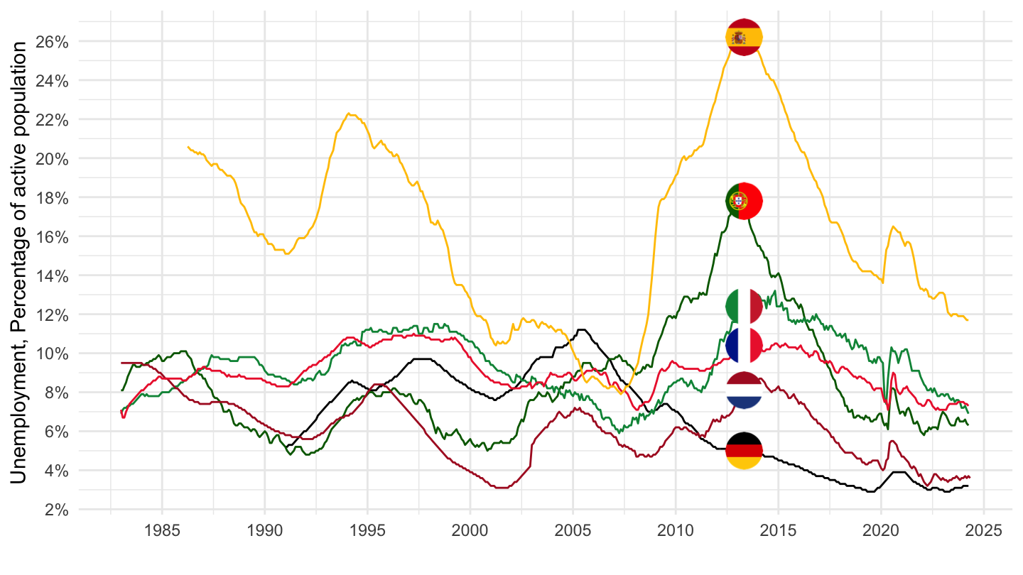
1998-
Code
une_rt_m %>%
  filter(geo %in% c("FR", "DE", "IT", "ES", "NL", "PT"),
         age == "TOTAL",
         sex == "T",
         unit == "PC_ACT",
         s_adj == "SA") %>%
  month_to_date %>%

  left_join(colors, by = c("Geo" = "country")) %>%
  mutate(values = values/100) %>%
  filter(date >= as.Date("1998-01-01")) %>%
  ggplot + geom_line(aes(x = date, y = values, color = color)) +
  theme_minimal() + scale_color_identity() + add_6flags +
  scale_x_date(breaks = as.Date(paste0(seq(1990, 2100, 4), "-01-01")),
               labels = date_format("%Y")) +
  xlab("") + ylab("Unemployment, Percentage of active population") +
  scale_y_continuous(breaks = 0.01*seq(0, 200, 2),
                     labels = scales::percent_format(accuracy = 1))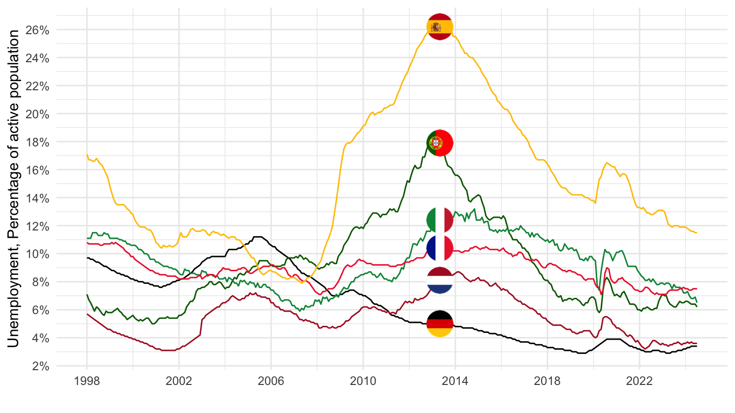
2014-
Code
une_rt_m %>%
  filter(geo %in% c("FR", "DE", "IT", "ES", "NL", "PT"),
         age == "TOTAL",
         sex == "T",
         unit == "PC_ACT",
         s_adj == "SA") %>%
  month_to_date %>%

  left_join(colors, by = c("Geo" = "country")) %>%
  mutate(values = values/100) %>%
  filter(date >= as.Date("2014-01-01")) %>%
  ggplot + geom_line(aes(x = date, y = values, color = color)) +
  theme_minimal() + scale_color_identity() + add_6flags +
  scale_x_date(breaks = as.Date(paste0(seq(1960, 2100, 1), "-01-01")),
               labels = date_format("%Y")) +
  xlab("") + ylab("Unemployment, Percentage of active population") +
  scale_y_continuous(breaks = 0.01*seq(0, 200, 2),
                     labels = scales::percent_format(accuracy = 1))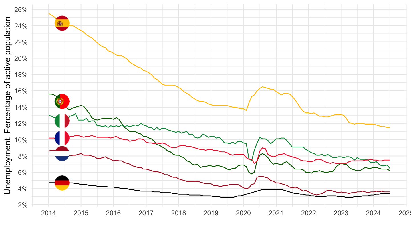
France, Germany, Portugal
Code
une_rt_m %>%
  filter(geo %in% c("FR", "DE", "PT"),
         age == "TOTAL",
         sex == "T",
         unit == "PC_ACT",
         s_adj == "SA") %>%
  month_to_date %>%

  left_join(colors, by = c("Geo" = "country")) %>%
  mutate(values = values/100) %>%
  ggplot + geom_line(aes(x = date, y = values, color = color)) +
  theme_minimal() + scale_color_identity() + add_3flags +
  scale_x_date(breaks = as.Date(paste0(seq(1960, 2100, 5), "-01-01")),
               labels = date_format("%Y")) +
  xlab("") + ylab("Unemployment, Percentage of active population") +
  scale_y_continuous(breaks = 0.01*seq(0, 200, 1),
                     labels = scales::percent_format(accuracy = 1))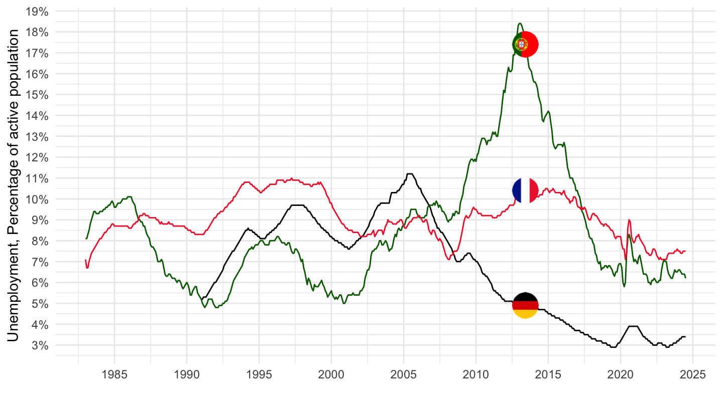
Germany, Euro Area
Code
une_rt_m %>%
  filter(geo %in% c("EA21", "EU15", "DE"),
         age == "TOTAL",
         sex == "T",
         unit == "PC_ACT",
         s_adj == "SA") %>%
  month_to_date %>%

  ggplot + geom_line() + theme_minimal()  +
  aes(x = date, y = values/100, color = Geo, linetype = Geo) +
  scale_color_manual(values = viridis(4)[1:3]) +
  scale_x_date(breaks = as.Date(paste0(seq(1960, 2100, 5), "-01-01")),
               labels = date_format("%Y")) +
  theme(legend.position = c(0.3, 0.25),
        legend.title = element_blank()) +
  xlab("") + ylab("Percentage of active population") +
  scale_y_continuous(breaks = 0.01*seq(0, 200, 1),
                     labels = scales::percent_format(accuracy = 1))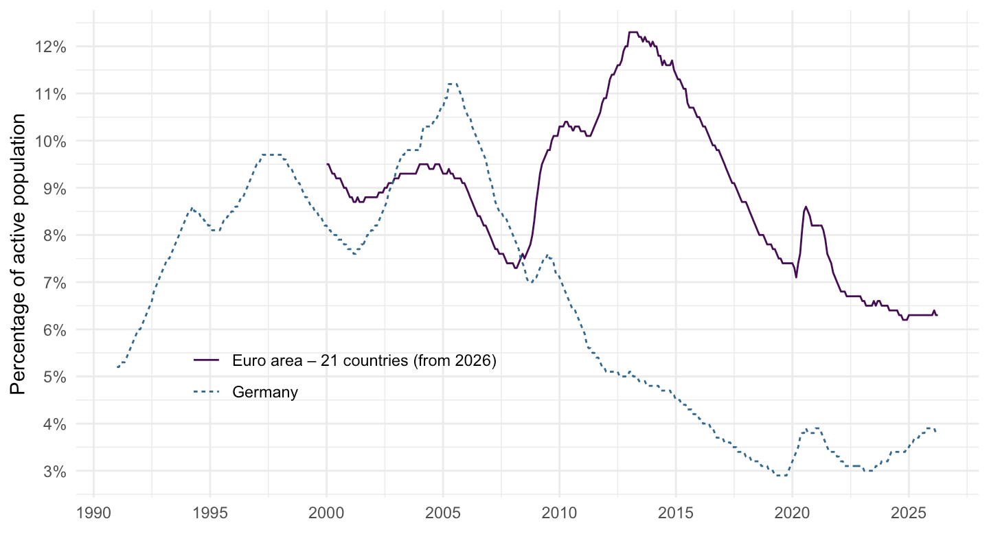
Spain, France
1998-
Code
une_rt_m %>%
  filter(geo %in% c("ES", "FR"),
         age == "TOTAL",
         sex == "T",
         unit == "PC_ACT",
         s_adj == "SA") %>%
  month_to_date %>%
  filter(date >= as.Date("1998-01-01")) %>%

  mutate(values = values/100,
         Geo = ifelse(geo == "EA21", "Europe", Geo)) %>%
  left_join(colors, by = c("Geo" = "country")) %>%
  ggplot + geom_line(aes(x = date, y = values, color = color)) +
  theme_minimal() + scale_color_identity() + add_2flags +
  scale_x_date(breaks = as.Date(paste0(seq(1998, 2100, 2), "-01-01")),
               labels = date_format("%Y")) +
  theme(legend.position = "none") +
  xlab("") + ylab("Unemployment, % of active population") +
  scale_y_continuous(breaks = 0.01*seq(0, 200, 1),
                     labels = scales::percent_format(accuracy = 1)) +
  geom_label(data = . %>%
                    filter(date == max(date)), aes(x = date, y = values, label = percent(values), color = color))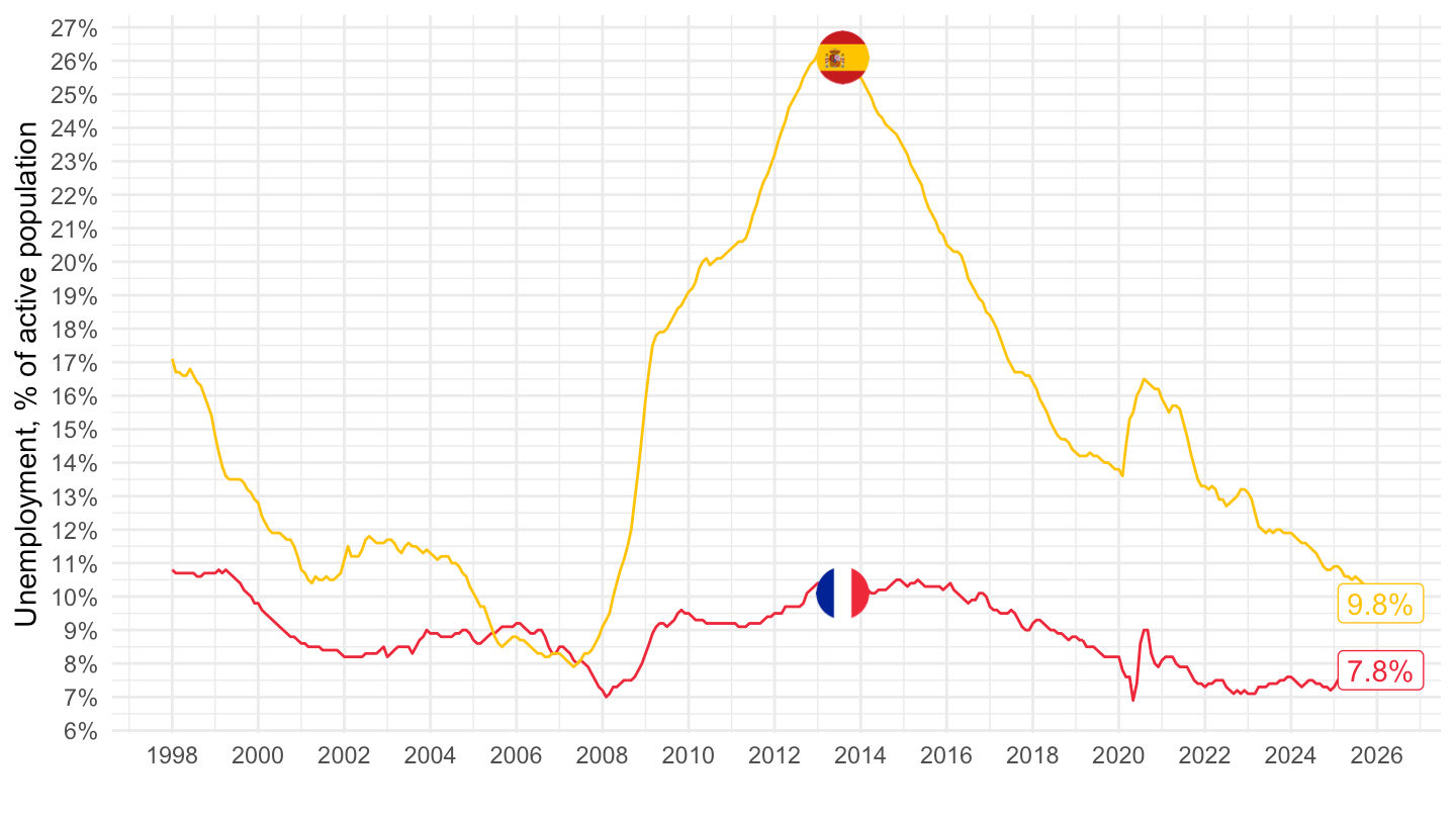
2010-
Code
une_rt_m %>%
  filter(geo %in% c("ES", "FR"),
         age == "TOTAL",
         sex == "T",
         unit == "PC_ACT",
         s_adj == "SA") %>%
  month_to_date %>%
  filter(date >= as.Date("2010-01-01")) %>%

  mutate(values = values/100,
         Geo = ifelse(geo == "EA21", "Europe", Geo)) %>%
  left_join(colors, by = c("Geo" = "country")) %>%
  ggplot + geom_line(aes(x = date, y = values, color = color)) +
  theme_minimal() + scale_color_identity() + add_2flags +
  scale_x_date(breaks = as.Date(paste0(seq(1960, 2100, 1), "-01-01")),
               labels = date_format("%Y")) +
  theme(legend.position = "none",
        axis.text.x = element_text(angle = 45, vjust = 1, hjust = 1)) +
  xlab("") + ylab("Unemployment, Percentage of active population") +
  scale_y_continuous(breaks = 0.01*seq(0, 200, .5),
                     labels = scales::percent_format(accuracy = .1)) +
  geom_text_repel(data = . %>%
                    filter(date == max(date)), aes(x = date, y = values, label = percent(values), color = color))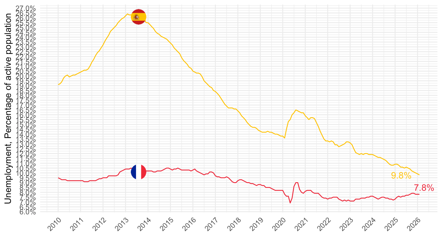
2017-
Code
une_rt_m %>%
  filter(geo %in% c("ES", "FR"),
         age == "TOTAL",
         sex == "T",
         unit == "PC_ACT",
         s_adj == "SA") %>%
  month_to_date %>%
  filter(date >= as.Date("2017-01-01")) %>%

  mutate(values = values/100,
         Geo = ifelse(geo == "EA21", "Europe", Geo)) %>%
  left_join(colors, by = c("Geo" = "country")) %>%
  ggplot + geom_line(aes(x = date, y = values, color = color)) +
  theme_minimal() + scale_color_identity() + add_2flags +
  scale_x_date(breaks = as.Date(paste0(seq(1960, 2100, 1), "-01-01")),
               labels = date_format("%Y")) +
  theme(legend.position = "none",
        axis.text.x = element_text(angle = 45, vjust = 1, hjust = 1)) +
  xlab("") + ylab("Unemployment, % of active population") +
  scale_y_continuous(breaks = 0.01*seq(0, 200, 1),
                     labels = scales::percent_format(accuracy = .1)) +
  geom_text_repel(data = . %>%
                    filter(date == max(date)), aes(x = date, y = values, label = percent(values), color = color))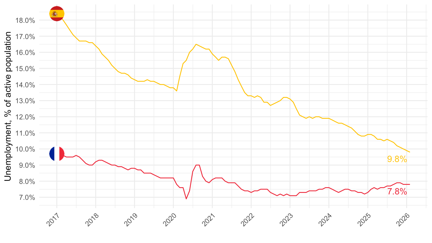
Euro Area, France
All
Code
une_rt_m %>%
  filter(geo %in% c("EA21", "FR"),
         age == "TOTAL",
         sex == "T",
         unit == "PC_ACT",
         s_adj == "SA") %>%
  month_to_date %>%

  mutate(values = values/100,
         Geo = ifelse(geo == "EA21", "Europe", Geo)) %>%
  left_join(colors, by = c("Geo" = "country")) %>%
  ggplot + geom_line(aes(x = date, y = values, color = color)) +
  theme_minimal() + scale_color_identity() + add_2flags +
  scale_x_date(breaks = as.Date(paste0(seq(1960, 2100, 5), "-01-01")),
               labels = date_format("%Y")) +
  theme(legend.position = "none") +
  xlab("") + ylab("Unemployment, Percentage of active population") +
  scale_y_continuous(breaks = 0.01*seq(0, 200, 1),
                     labels = scales::percent_format(accuracy = 1))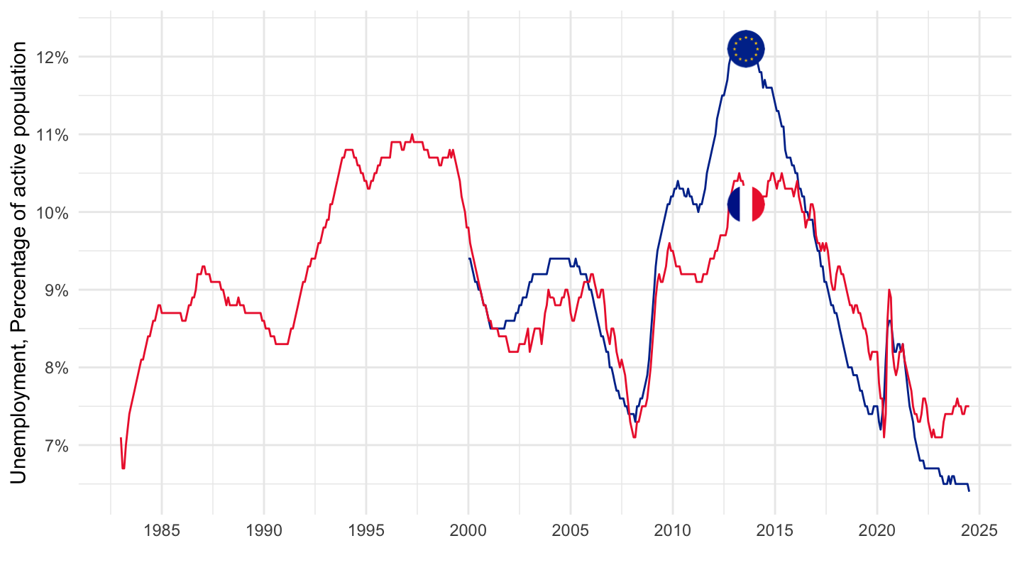
1998-
Code
une_rt_m %>%
  filter(geo %in% c("EA21", "FR"),
         age == "TOTAL",
         sex == "T",
         unit == "PC_ACT",
         s_adj == "SA") %>%
  month_to_date %>%
  filter(date >= as.Date("1998-01-01")) %>%

  mutate(values = values/100,
         Geo = ifelse(geo == "EA21", "Europe", Geo)) %>%
  left_join(colors, by = c("Geo" = "country")) %>%
  ggplot + geom_line(aes(x = date, y = values, color = color)) +
  theme_minimal() + scale_color_identity() + add_2flags +
  scale_x_date(breaks = as.Date(paste0(seq(1998, 2100, 2), "-01-01")),
               labels = date_format("%Y")) +
  theme(legend.position = "none") +
  xlab("") + ylab("Unemployment, % of active population") +
  scale_y_continuous(breaks = 0.01*seq(0, 200, 1),
                     labels = scales::percent_format(accuracy = 1)) +
  geom_label(data = . %>%
                    filter(date == max(date)), aes(x = date, y = values, label = percent(values), color = color))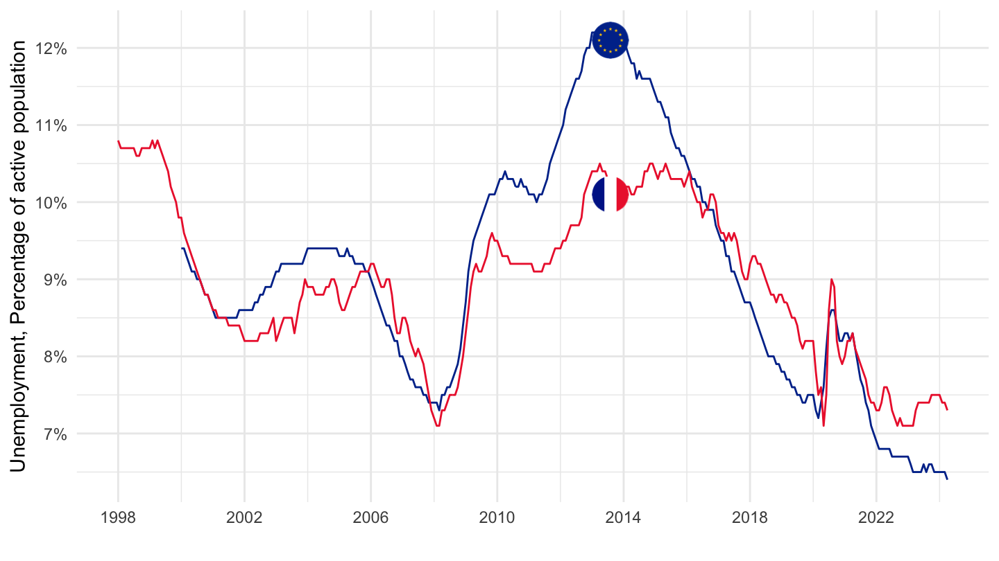
2010-
Code
une_rt_m %>%
  filter(geo %in% c("EA21", "FR"),
         age == "TOTAL",
         sex == "T",
         unit == "PC_ACT",
         s_adj == "SA") %>%
  month_to_date %>%
  filter(date >= as.Date("2010-01-01")) %>%

  mutate(values = values/100,
         Geo = ifelse(geo == "EA21", "Europe", Geo)) %>%
  left_join(colors, by = c("Geo" = "country")) %>%
  ggplot + geom_line(aes(x = date, y = values, color = color)) +
  theme_minimal() + scale_color_identity() + add_2flags +
  scale_x_date(breaks = as.Date(paste0(seq(1960, 2100, 1), "-01-01")),
               labels = date_format("%Y")) +
  theme(legend.position = "none",
        axis.text.x = element_text(angle = 45, vjust = 1, hjust = 1)) +
  xlab("") + ylab("Unemployment, Percentage of active population") +
  scale_y_continuous(breaks = 0.01*seq(0, 200, .5),
                     labels = scales::percent_format(accuracy = .1)) +
  geom_text_repel(data = . %>%
                    filter(date == max(date)), aes(x = date, y = values, label = percent(values), color = color))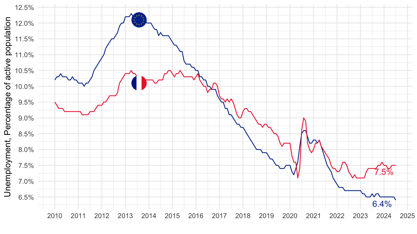
Euro Area, France, Spain
All
Code
une_rt_m %>%
  filter(geo %in% c("EA21", "FR", "ES"),
         age == "TOTAL",
         sex == "T",
         unit == "PC_ACT",
         s_adj == "SA") %>%
  month_to_date %>%

  mutate(values = values/100,
         Geo = ifelse(geo == "EA21", "Europe", Geo)) %>%
  left_join(colors, by = c("Geo" = "country")) %>%
  ggplot + geom_line(aes(x = date, y = values, color = color)) +
  theme_minimal() + scale_color_identity() + add_3flags +
  scale_x_date(breaks = as.Date(paste0(seq(1960, 2100, 5), "-01-01")),
               labels = date_format("%Y")) +
  theme(legend.position = "none") +
  xlab("") + ylab("Unemployment, Percentage of active population") +
  scale_y_continuous(breaks = 0.01*seq(0, 200, 1),
                     labels = scales::percent_format(accuracy = 1))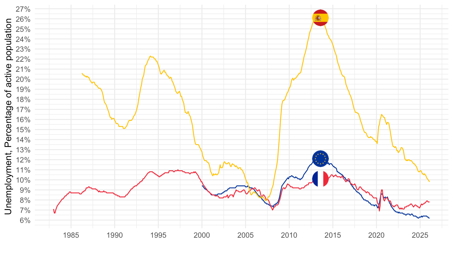
1998-
Code
une_rt_m %>%
  filter(geo %in% c("EA21", "FR", "ES"),
         age == "TOTAL",
         sex == "T",
         unit == "PC_ACT",
         s_adj == "SA") %>%
  month_to_date %>%
  filter(date >= as.Date("1998-01-01")) %>%

  mutate(values = values/100,
         Geo = ifelse(geo == "EA21", "Europe", Geo)) %>%
  left_join(colors, by = c("Geo" = "country")) %>%
  ggplot + geom_line(aes(x = date, y = values, color = color)) +
  theme_minimal() + scale_color_identity() + add_3flags +
  scale_x_date(breaks = as.Date(paste0(seq(1998, 2100, 2), "-01-01")),
               labels = date_format("%Y")) +
  theme(legend.position = "none") +
  xlab("") + ylab("Unemployment, % of active population") +
  scale_y_continuous(breaks = 0.01*seq(0, 200, 1),
                     labels = scales::percent_format(accuracy = 1)) +
  geom_label(data = . %>%
                    filter(date == max(date)), aes(x = date, y = values, label = percent(values), color = color))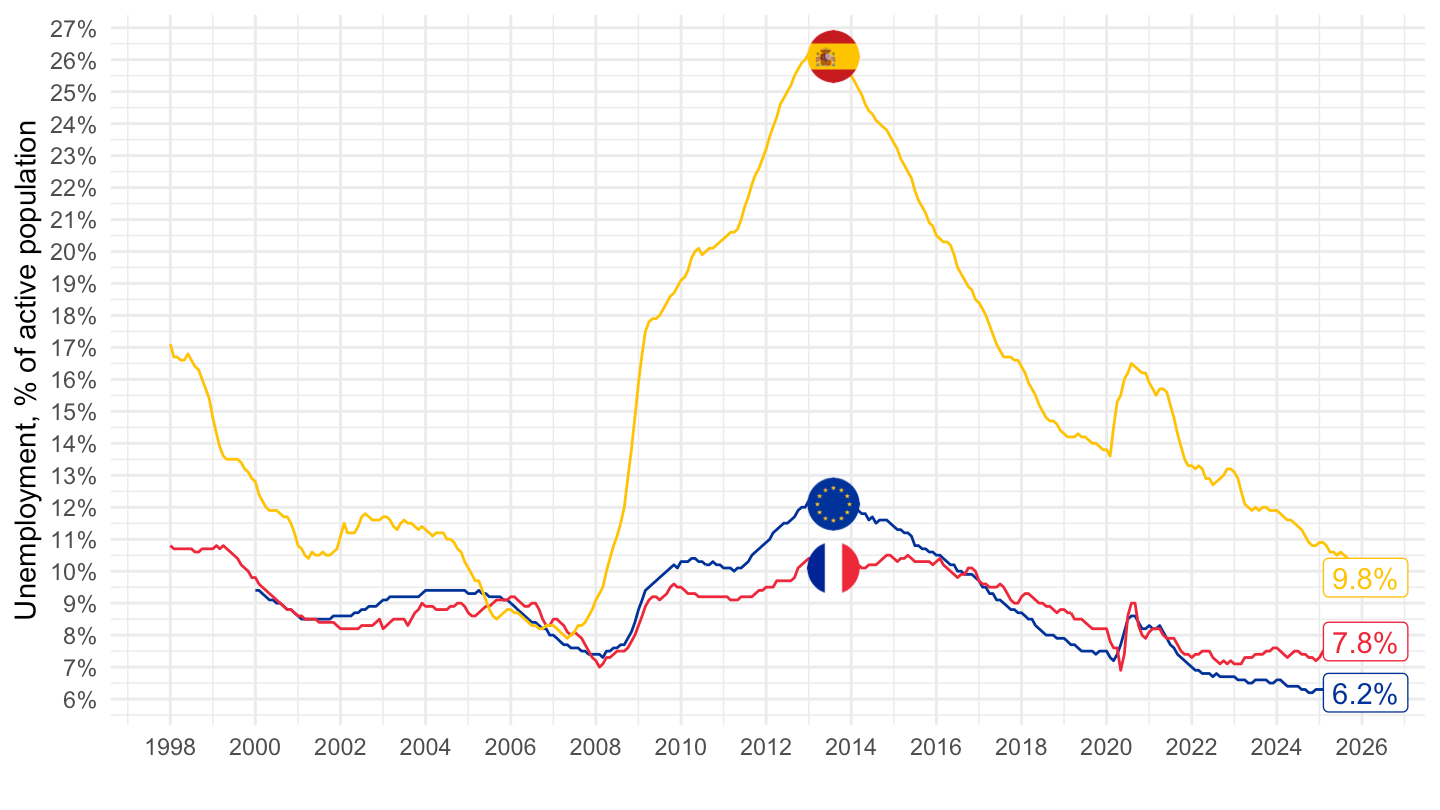
2010-
Code
une_rt_m %>%
  filter(geo %in% c("EA21", "FR","ES"),
         age == "TOTAL",
         sex == "T",
         unit == "PC_ACT",
         s_adj == "SA") %>%
  month_to_date %>%
  filter(date >= as.Date("2010-01-01")) %>%

  mutate(values = values/100,
         Geo = ifelse(geo == "EA21", "Europe", Geo)) %>%
  left_join(colors, by = c("Geo" = "country")) %>%
  ggplot + geom_line(aes(x = date, y = values, color = color)) +
  theme_minimal() + scale_color_identity() + add_3flags +
  scale_x_date(breaks = as.Date(paste0(seq(1960, 2100, 1), "-01-01")),
               labels = date_format("%Y")) +
  theme(legend.position = "none",
        axis.text.x = element_text(angle = 45, vjust = 1, hjust = 1)) +
  xlab("") + ylab("Unemployment, Percentage of active population") +
  scale_y_continuous(breaks = 0.01*seq(0, 200, .5),
                     labels = scales::percent_format(accuracy = .1)) +
  geom_text_repel(data = . %>%
                    filter(date == max(date)), aes(x = date, y = values, label = percent(values), color = color))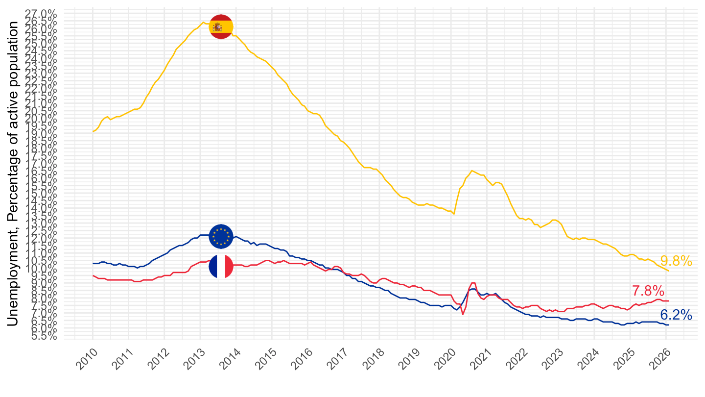
2017-
Code
une_rt_m %>%
  filter(geo %in% c("EA21", "FR","ES"),
         age == "TOTAL",
         sex == "T",
         unit == "PC_ACT",
         s_adj == "SA") %>%
  month_to_date %>%
  filter(date >= as.Date("2017-01-01")) %>%

  mutate(values = values/100,
         Geo = ifelse(geo == "EA21", "Europe", Geo)) %>%
  left_join(colors, by = c("Geo" = "country")) %>%
  ggplot + geom_line(aes(x = date, y = values, color = color)) +
  theme_minimal() + scale_color_identity() + add_3flags +
  scale_x_date(breaks = as.Date(paste0(seq(1960, 2100, 1), "-01-01")),
               labels = date_format("%Y")) +
  theme(legend.position = "none",
        axis.text.x = element_text(angle = 45, vjust = 1, hjust = 1)) +
  xlab("") + ylab("Unemployment, % of active population") +
  scale_y_continuous(breaks = 0.01*seq(0, 200, .5),
                     labels = scales::percent_format(accuracy = .1)) +
  geom_text_repel(data = . %>%
                    filter(date == max(date)), aes(x = date, y = values, label = percent(values), color = color))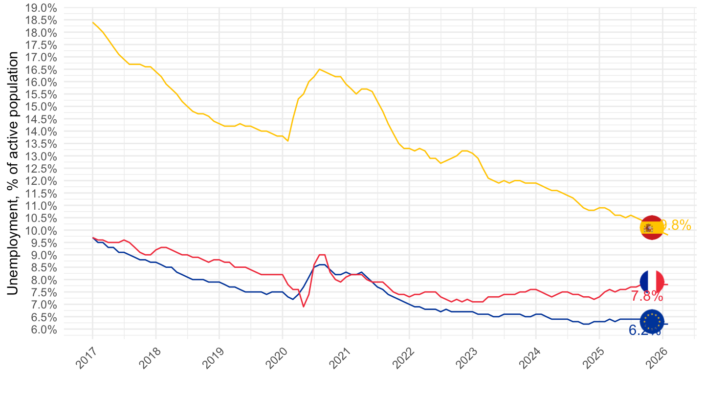
Euro Area, Bulgaria
All
Code
une_rt_m %>%
  filter(geo %in% c("EA21", "BG"),
         age == "TOTAL",
         sex == "T",
         unit == "PC_ACT",
         s_adj == "SA") %>%
  month_to_date %>%

  mutate(values = values/100,
         Geo = ifelse(geo == "EA21", "Europe", Geo)) %>%
  left_join(colors, by = c("Geo" = "country")) %>%
  ggplot + geom_line(aes(x = date, y = values, color = color)) +
  theme_minimal() + scale_color_identity() + add_2flags +
  scale_x_date(breaks = as.Date(paste0(seq(1960, 2100, 5), "-01-01")),
               labels = date_format("%Y")) +
  theme(legend.position = "none") +
  xlab("") + ylab("Unemployment, Percentage of active population") +
  scale_y_continuous(breaks = 0.01*seq(0, 200, 1),
                     labels = scales::percent_format(accuracy = 1))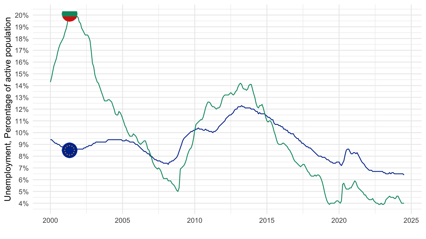
2010-
Code
une_rt_m %>%
  filter(geo %in% c("EA21", "BG"),
         age == "TOTAL",
         sex == "T",
         unit == "PC_ACT",
         s_adj == "SA") %>%
  month_to_date %>%
  filter(date >= as.Date("2010-01-01")) %>%

  mutate(values = values/100,
         Geo = ifelse(geo == "EA21", "Europe", Geo)) %>%
  left_join(colors, by = c("Geo" = "country")) %>%
  ggplot + geom_line(aes(x = date, y = values, color = color)) +
  theme_minimal() + scale_color_identity() + add_2flags +
  scale_x_date(breaks = as.Date(paste0(seq(1960, 2100, 1), "-01-01")),
               labels = date_format("%Y")) +
  theme(legend.position = "none",
        axis.text.x = element_text(angle = 45, vjust = 1, hjust = 1)) +
  xlab("") + ylab("Unemployment, Percentage of active population") +
  scale_y_continuous(breaks = 0.01*seq(0, 200, 1),
                     labels = scales::percent_format(accuracy = 1))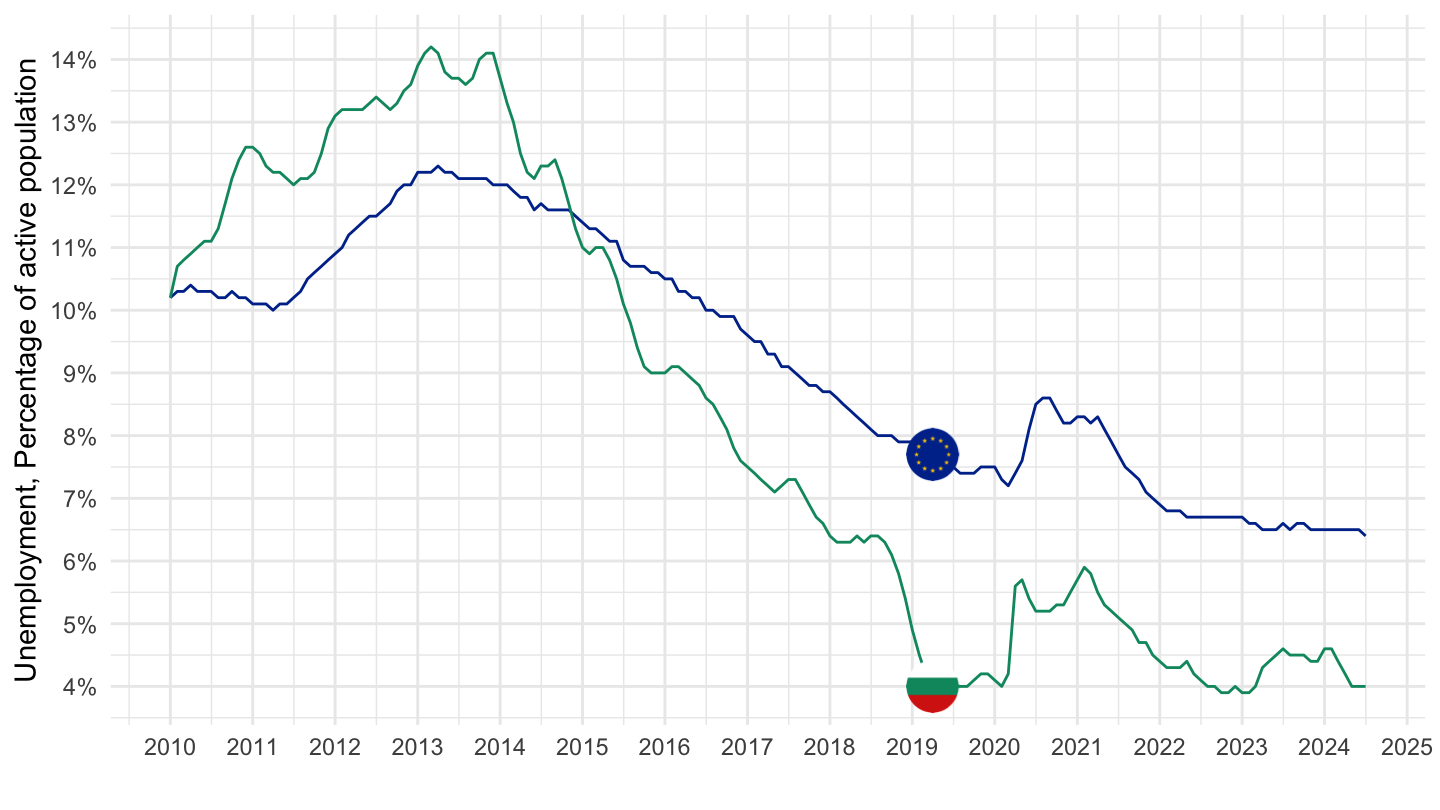
By age
Euro Area
Code
une_rt_m %>%
  filter(geo %in% c("EA21"),
         sex == "T",
         unit == "PC_ACT",
         s_adj == "SA") %>%
  month_to_date %>%

  ggplot + geom_line() + theme_minimal()  +
  aes(x = date, y = values/100, color = Age) +
  scale_x_date(breaks = as.Date(paste0(seq(1960, 2100, 5), "-01-01")),
               labels = date_format("%Y")) +
  theme(legend.position = c(0.2, 0.85),
        legend.title = element_blank()) +
  xlab("") + ylab("Percentage of active population") +
  scale_y_continuous(breaks = 0.01*seq(0, 200, 1),
                     labels = scales::percent_format(accuracy = 1))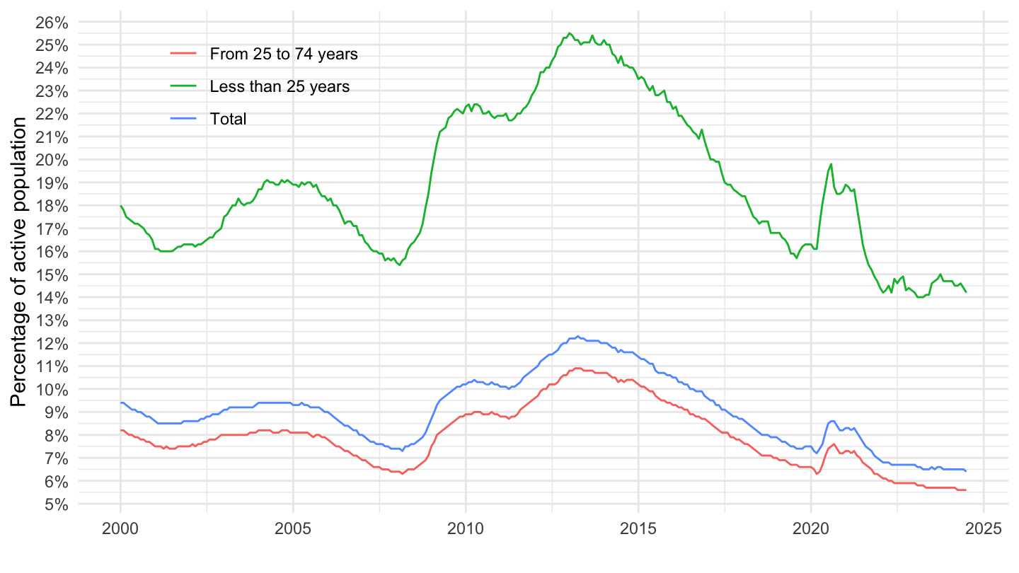
France
Code
une_rt_m %>%
  filter(geo == "FR",
         sex == "T",
         unit == "PC_ACT",
         s_adj == "SA") %>%
  month_to_date %>%

  ggplot + geom_line() + theme_minimal()  +
  aes(x = date, y = values/100, color = Age) +
  scale_x_date(breaks = as.Date(paste0(seq(1960, 2100, 5), "-01-01")),
               labels = date_format("%Y")) +
  theme(legend.position = c(0.2, 0.85),
        legend.title = element_blank()) +
  xlab("") + ylab("Percentage of active population") +
  scale_y_continuous(breaks = 0.01*seq(0, 200, 1),
                     labels = scales::percent_format(accuracy = 1))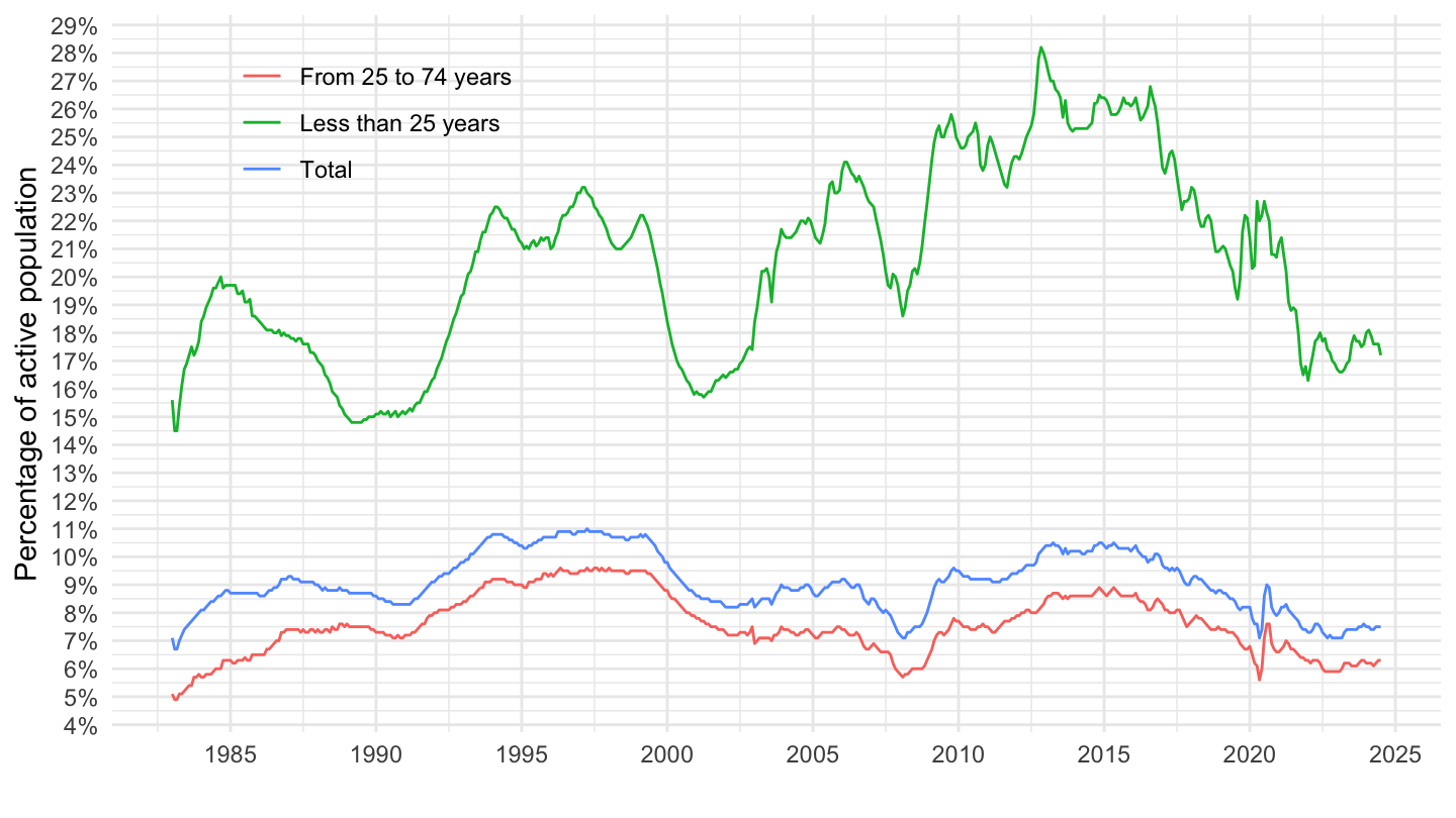
Germany
Code
une_rt_m %>%
  filter(geo == "DE",
         sex == "T",
         unit == "PC_ACT",
         s_adj == "SA") %>%
  month_to_date %>%

  ggplot + geom_line() + theme_minimal()  +
  aes(x = date, y = values/100, color = Age) +
  scale_x_date(breaks = as.Date(paste0(seq(1960, 2100, 5), "-01-01")),
               labels = date_format("%Y")) +
  theme(legend.position = c(0.2, 0.85),
        legend.title = element_blank()) +
  xlab("") + ylab("Percentage of active population") +
  scale_y_continuous(breaks = 0.01*seq(0, 200, 1),
                     labels = scales::percent_format(accuracy = 1))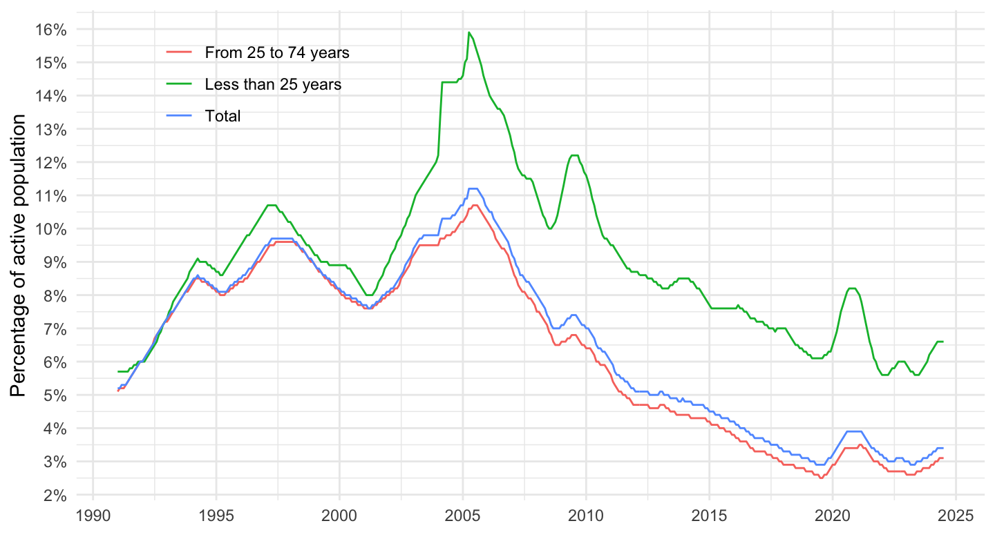
By sex
Euro Area
Code
une_rt_m %>%
  filter(geo %in% c("EA21"),
         age == "TOTAL",
         unit == "PC_ACT",
         s_adj == "SA") %>%
  month_to_date %>%

  ggplot + geom_line() + theme_minimal()  +
  aes(x = date, y = values/100, color = Sex) +
  scale_x_date(breaks = as.Date(paste0(seq(1960, 2100, 2), "-01-01")),
               labels = date_format("%Y")) +
  theme(legend.position = c(0.2, 0.85),
        legend.title = element_blank()) +
  xlab("") + ylab("Percentage of active population") +
  scale_y_continuous(breaks = 0.01*seq(0, 200, 1),
                     labels = scales::percent_format(accuracy = 1))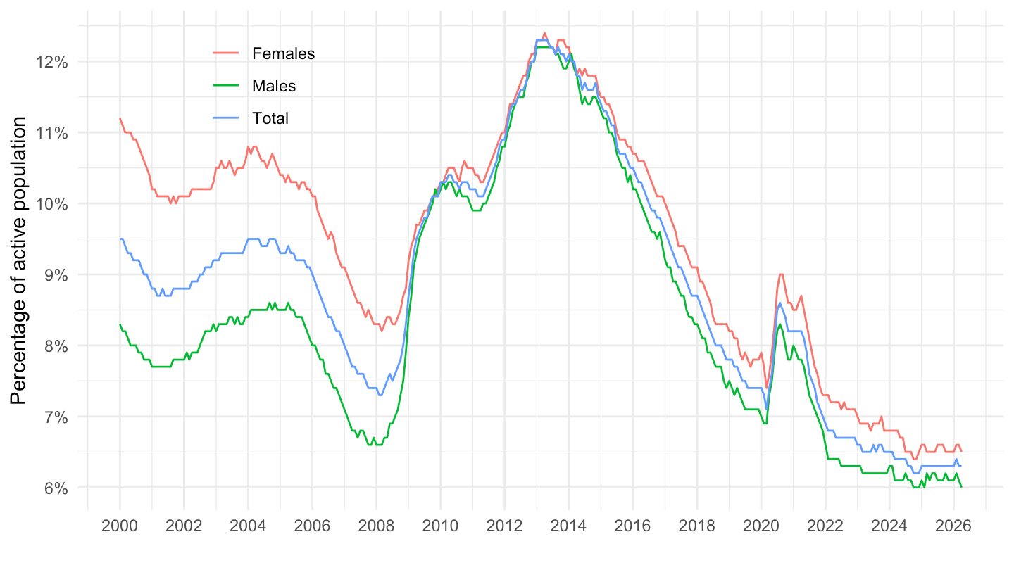
France
Code
une_rt_m %>%
  filter(geo == "FR",
         age == "TOTAL",
         unit == "PC_ACT",
         s_adj == "SA") %>%
  month_to_date %>%

  ggplot + geom_line() + theme_minimal()  +
  aes(x = date, y = values/100, color = Sex) +
  scale_x_date(breaks = as.Date(paste0(seq(1960, 2100, 5), "-01-01")),
               labels = date_format("%Y")) +
  theme(legend.position = c(0.6, 0.85),
        legend.title = element_blank()) +
  xlab("") + ylab("Percentage of active population") +
  scale_y_continuous(breaks = 0.01*seq(0, 200, 1),
                     labels = scales::percent_format(accuracy = 1))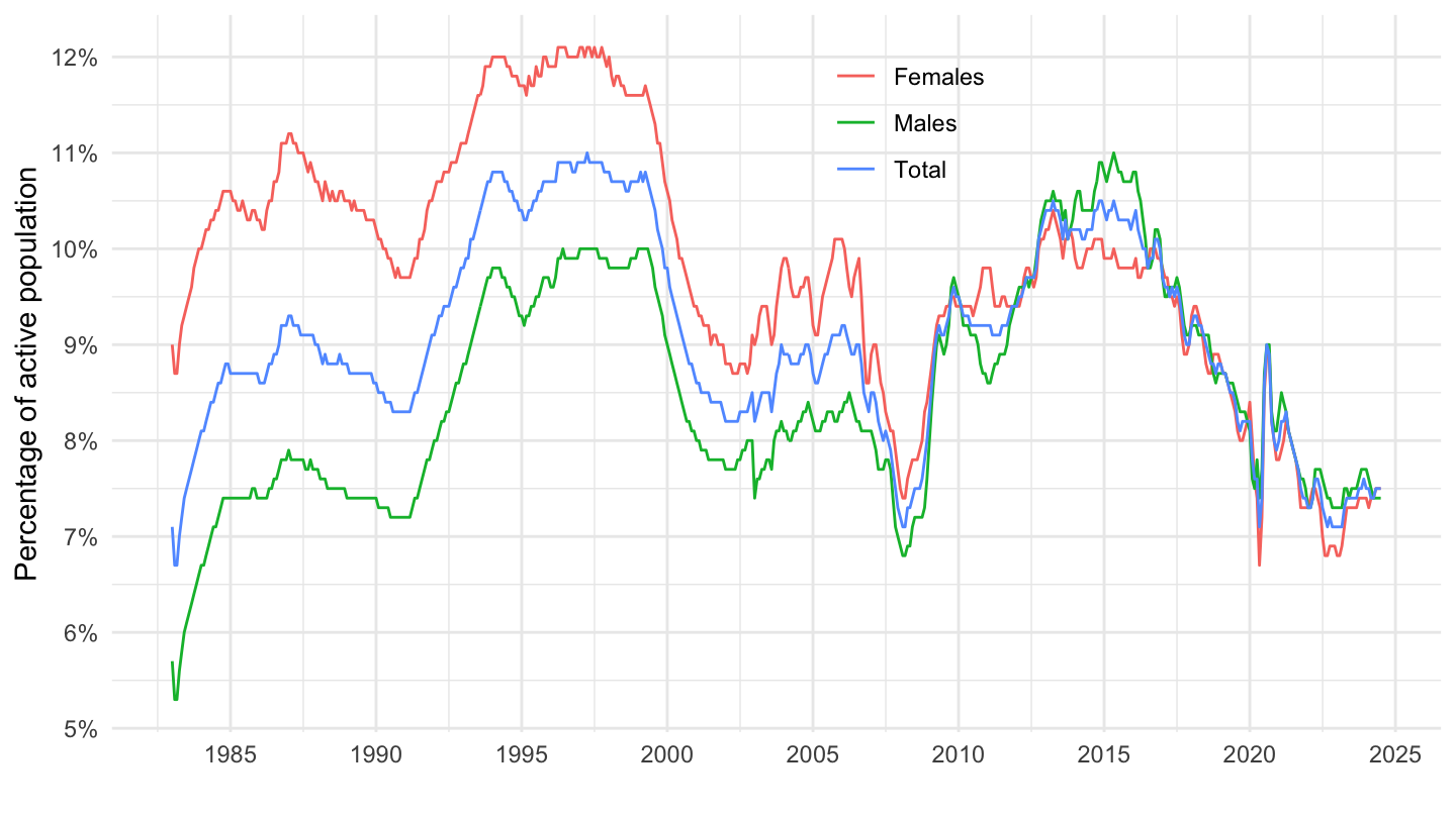
Germany
Code
une_rt_m %>%
  filter(geo == "DE",
         age == "TOTAL",
         unit == "PC_ACT",
         s_adj == "SA") %>%
  month_to_date %>%

  ggplot + geom_line() + theme_minimal()  +
  aes(x = date, y = values/100, color = Sex) +
  scale_x_date(breaks = as.Date(paste0(seq(1960, 2100, 5), "-01-01")),
               labels = date_format("%Y")) +
  theme(legend.position = c(0.8, 0.85),
        legend.title = element_blank()) +
  xlab("") + ylab("Percentage of active population") +
  scale_y_continuous(breaks = 0.01*seq(0, 200, 1),
                     labels = scales::percent_format(accuracy = 1))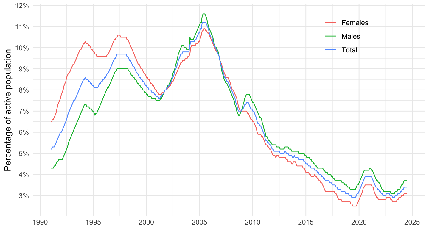
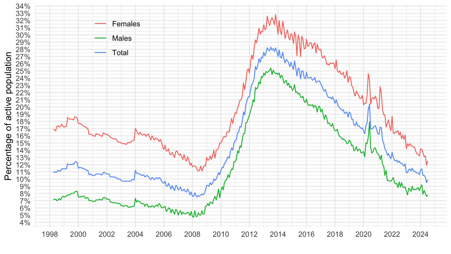
Italy
Code
une_rt_m %>%
  filter(geo == "IT",
         age == "TOTAL",
         unit == "PC_ACT",
         s_adj == "SA") %>%
  month_to_date %>%

  ggplot + geom_line() + theme_minimal()  +
  aes(x = date, y = values/100, color = Sex) +
  scale_x_date(breaks = as.Date(paste0(seq(1960, 2100, 5), "-01-01")),
               labels = date_format("%Y")) +
  theme(legend.position = c(0.6, 0.85),
        legend.title = element_blank()) +
  xlab("") + ylab("Percentage of active population") +
  scale_y_continuous(breaks = 0.01*seq(0, 200, 1),
                     labels = scales::percent_format(accuracy = 1))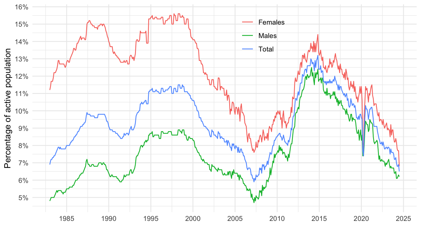
Greece
Code
une_rt_m %>%
  filter(geo == "EL",
         age == "TOTAL",
         unit == "PC_ACT",
         s_adj == "SA") %>%
  month_to_date %>%

  ggplot + geom_line() + theme_minimal()  +
  aes(x = date, y = values/100, color = Sex) +
  scale_x_date(breaks = as.Date(paste0(seq(1960, 2100, 2), "-01-01")),
               labels = date_format("%Y")) +
  theme(legend.position = c(0.2, 0.85),
        legend.title = element_blank()) +
  xlab("") + ylab("Percentage of active population") +
  scale_y_continuous(breaks = 0.01*seq(0, 200, 1),
                     labels = scales::percent_format(accuracy = 1))