Last compile: 10 oct. 2026, 00:01
LAST_COMPILE
| LAST_COMPILE |
|---|
| 2026-10-10 |
Last
| date | Nobs |
|---|---|
| 2026-08-01 | 310 |
la.area
All
Code
la.area |>
  select(2, 3) |>
  print_table_conditional()
State
Code
la.area |>
  filter(area_type_code == "A") |>
  select(2, 3) |>
  print_table_conditional()
Metropolitan areas
Code
la.area |>
  filter(area_type_code == "B") |>
  select(2, 3) |>
  print_table_conditional()
Metropolitan divisions
Code
la.area |>
  filter(area_type_code == "C") |>
  select(2, 3) |>
  print_table_conditional()
Micropolitan areas
Code
la.area |>
  filter(area_type_code == "D") |>
  select(2, 3) |>
  print_table_conditional()
Combined areas
Code
la.area |>
  filter(area_type_code == "E") |>
  select(2, 3) |>
  print_table_conditional()
Counties and equivalents
Code
la.area |>
  filter(area_type_code == "F") |>
  select(2, 3) |>
  print_table_conditional()
Cities and towns above 25,000 population
Code
la.area |>
  filter(area_type_code == "G") |>
  select(2, 3) |>
  print_table_conditional()
Cities and towns below 25,000 population in New England
Code
la.area |>
  filter(area_type_code == "H") |>
  select(2, 3) |>
  print_table_conditional()
Parts of cities that cross county boundaries
Code
la.area |>
  filter(area_type_code == "I") |>
  select(2, 3) |>
  print_table_conditional()
Multi-entity small labor market areas
Code
la.area |>
  filter(area_type_code == "J") |>
  select(2, 3) |>
print_table_conditional()| area_code | area_text |
|---|---|
| SA0881220000000 | Gunnison-Hinsdale, CO LMA |
| SA0882100000000 | Otero-Crowley, CO LMA |
| SA1381140000000 | Greene-Taliaferro, GA LMA |
| SA1382780000000 | Telfair-Wheeler, GA LMA |
| SA1681460000000 | Idaho-Lewis, ID LMA |
| SA1682820000000 | Valley-Adams, ID LMA |
| SA2182180000000 | Perry-Knott, KY LMA |
| SA2282860000000 | West Carroll-East Carroll, LA LMA |
| SA2782140000000 | Pennington-Red Lake, MN LMA |
| SA2882620000000 | Sharkey-Issaquena, MS LMA |
| SA3182500000000 | Red Willow-Hitchcock, NE LMA |
| SA4680860000000 | Dewey-Ziebach, SD LMA |
| SA4880260000000 | Burnet-Llano, TX LMA |
| SA4880780000000 | Dallam-Hartley, TX LMA |
| SA4880820000000 | Dawson-Borden, TX LMA |
| SA4881500000000 | Jasper-Newton, TX LMA |
| SA4982580000000 | Sevier-Piute, UT LMA |
| SA5180180000000 | Alleghany-Covington, VA LMA |
| SA5180580000000 | Carroll-Galax, VA LMA |
| SA5181180000000 | Greensville-Emporia, VA LMA |
| SA5182540000000 | Rockbridge-Lexington-Buena Vista, VA LMA |
| SA5182740000000 | Southampton-Franklin, VA LMA |
| SA5182900000000 | Wise-Norton, VA LMA |
| SA5481260000000 | Hardy-Grant, WV LMA |
| SA5580220000000 | Ashland-Bayfield, WI LMA |
Intrastate parts of interstate areas
Code
la.area |>
  filter(area_type_code == "K") |>
  select(2, 3) |>
  print_table_conditional()
Balance of state areas
Code
la.area |>
  filter(area_type_code == "L") |>
  select(2, 3) |>
print_table_conditional()| area_code | area_text |
|---|---|
| BS0600000000000 | Balance of California, state less Los Angeles-Long Beach-Glendale MD |
| BS1200000000000 | Balance of Florida, state less Miami-Miami Beach-Kendall MD |
| BS1700000000000 | Balance of Illinois, state less Chicago-Naperville-Schaumburg MD |
| BS2600000000000 | Balance of Michigan, state less Detroit-Warren-Dearborn MSA |
| BS3600000000000 | Balance of New York, state less New York city |
| BS3900000000000 | Balance of Ohio, state less Cleveland MSA |
| BS5300000000000 | Balance of Washington, state less Seattle-Tacoma-Bellevue MSA |
Census regions
Code
la.area |>
  filter(area_type_code == "M") |>
  select(2, 3) |>
print_table_conditional()| area_code | area_text |
|---|---|
| RD9100000000000 | Northeast region |
| RD9200000000000 | Midwest region |
| RD9300000000000 | South region |
| RD9400000000000 | West region |
Census divisions
Code
la.area |>
  filter(area_type_code == "N") |>
  select(2, 3) |>
print_table_conditional()| area_code | area_text |
|---|---|
| RD8100000000000 | New England division |
| RD8200000000000 | Middle Atlantic division |
| RD8300000000000 | East North Central division |
| RD8400000000000 | West North Central division |
| RD8500000000000 | South Atlantic division |
| RD8600000000000 | East South Central division |
| RD8700000000000 | West South Central division |
| RD8800000000000 | Mountain division |
| RD8900000000000 | Pacific division |
la.area_type
Code
la.area_type |>
print_table_conditional()| area_type_code | areatype_text |
|---|---|
| A | Statewide |
| B | Metropolitan areas |
| C | Metropolitan divisions |
| D | Micropolitan areas |
| E | Combined areas |
| F | Counties and equivalents |
| G | Cities and towns above 25,000 population |
| H | Cities and towns below 25,000 population in New England |
| I | Parts of cities that cross county boundaries |
| J | Multi-entity small labor market areas |
| K | Intrastate parts of interstate areas |
| L | Balance of state areas |
| M | Census regions |
| N | Census divisions |
la.state_region_division
Code
la.state_region_division |>
  print_table_conditional()
la.measure
Code
la.measure |>
print_table_conditional()| measure_code | measure_text |
|---|---|
| 3 | unemployment rate |
| 4 | unemployment |
| 5 | employment |
| 6 | labor force |
| 7 | employment-population ratio |
| 8 | labor force participation rate |
| 9 | civilian noninstitutional population |
la.seasonal
Code
la.seasonal |>
print_table_conditional()| seasonal_code | seasonal_text |
|---|---|
| S | Seasonally Adjusted |
| U | Not Seasonally Adjusted |
Longest Series
Code
la.series |>
  arrange(begin_year) |>
  head(100) |>
  select(series_id, series_title, begin_year, end_year) |>
  print_table_conditional()
State
Arkansas, California, Nevada
Code
la.data.3.AllStatesS |>
  left_join(la.series, by = "series_id") |>
  left_join(la.area, by = c("area_code", "area_type_code")) |>
  filter(measure_code == 3,
         area_type_code == "A",
         area_text %in% c("California", "Arkansas", "Nevada")) |>
  month_to_date() |>
  #filter(date <= as.Date("2020-01-01")) %>%
  ggplot() + theme_minimal() + xlab("") + ylab("") +
  geom_line(aes(x = date, y = value / 100, color = area_text)) +
  theme(legend.position = c(0.10, 0.85),
        legend.title = element_blank()) +

  scale_x_date(breaks = as.Date(paste0(seq(1970, 2100, 5), "-01-01")),
               labels = date_format("%Y")) +
  scale_y_continuous(breaks = 0.01*seq(0, 100, 1),
                     labels = scales::percent_format(accuracy = 1))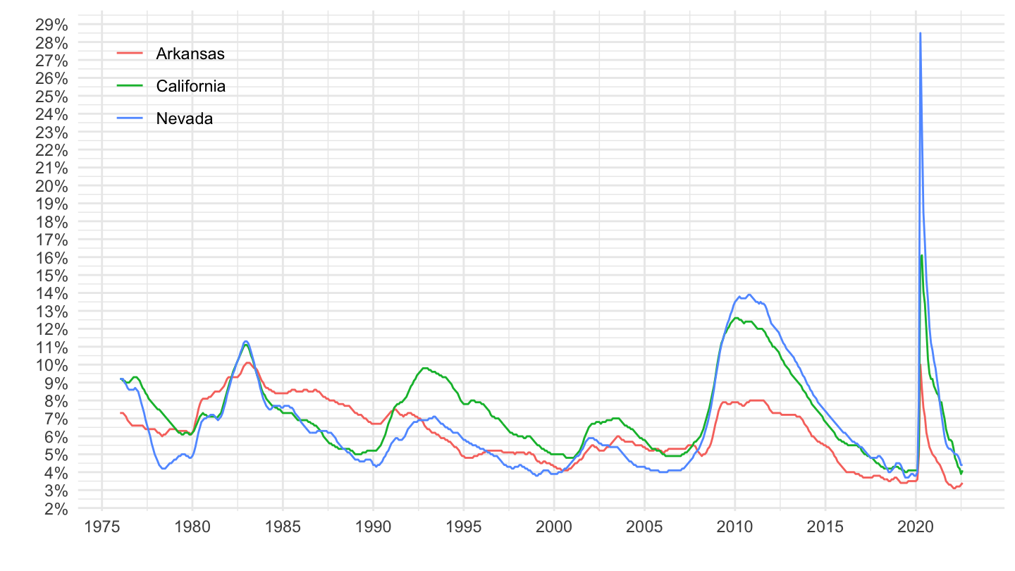
Metropolitan
Abilene, Akron
Code
la.data.60.Metro |>
  left_join(la.series, by = "series_id") |>
  left_join(la.measure, by = "measure_code") |>
  select(-area_type_code) |>
  left_join(la.area, by = "area_code") |>
  left_join(la.area_type, by = "area_type_code") |>
  filter(measure_text == "unemployment rate",
         area_type_code == "B",
         area_text %in% c("Abilene, TX Metropolitan Statistical Area",
                          "Akron, OH Metropolitan Statistical Area")) |>
  month_to_date() |>
  ggplot() + theme_minimal() + xlab("") + ylab("") +
  geom_line(aes(x = date, y = as.numeric(value) / 100, color = area_text)) +
  theme(legend.position = c(0.30, 0.85),
        legend.title = element_blank()) +

  scale_y_continuous(breaks = 0.01*seq(0, 100, 1),
                     labels = scales::percent_format(accuracy = 1)) +
  scale_x_date(breaks = as.Date(paste0(seq(1970, 2100, 5), "-01-01")),
               labels = date_format("%Y"))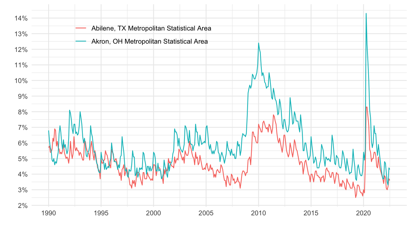
Combined
Los Angeles
Code
la.data.63.Combined |>
  left_join(la.series, by = "series_id") |>
  left_join(la.measure, by = "measure_code") |>
  select(-area_type_code) |>
  left_join(la.area, by = "area_code") |>
  left_join(la.area_type, by = "area_type_code") |>
  filter(measure_text == "unemployment rate",
         area_type_code == "E",
         grepl("Los Angeles", area_text) |
           grepl("New York", area_text) |
           grepl("Chicago", area_text)) |>
  month_to_date() |>
  #filter(date <= as.Date("2020-01-01")) %>%
  ggplot() + theme_minimal() + xlab("") + ylab("") +
  geom_line(aes(x = date, y = as.numeric(value) / 100, color = area_text)) +

  theme(legend.position = c(0.30, 0.85),
        legend.title = element_blank()) +
  scale_y_continuous(breaks = 0.01*seq(0, 100, 1),
                     labels = scales::percent_format(accuracy = 1)) +
  scale_x_date(breaks = as.Date(paste0(seq(1970, 2100, 5), "-01-01")),
               labels = date_format("%Y"))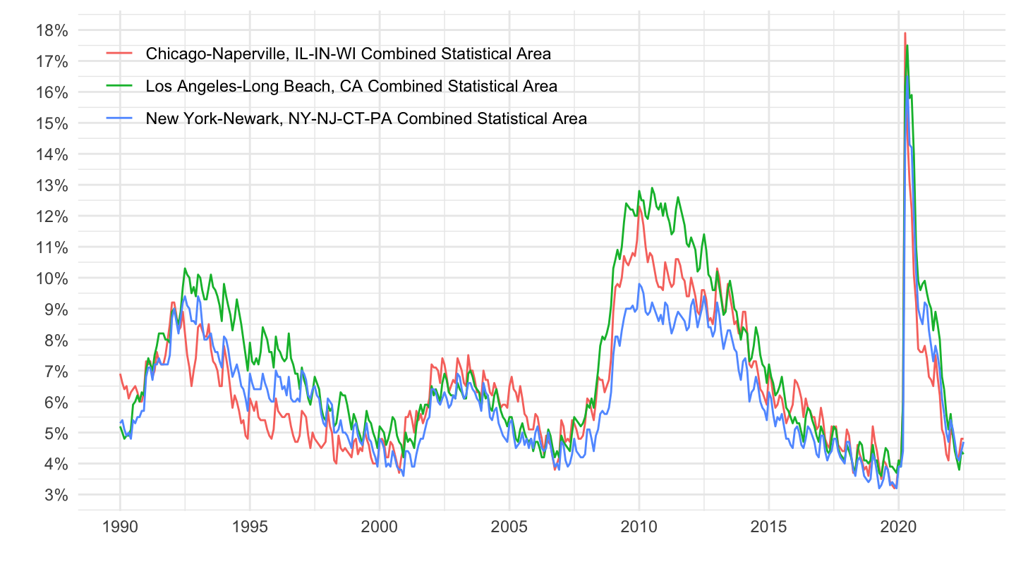
Cross-Section
U.S. MSAs
99-06
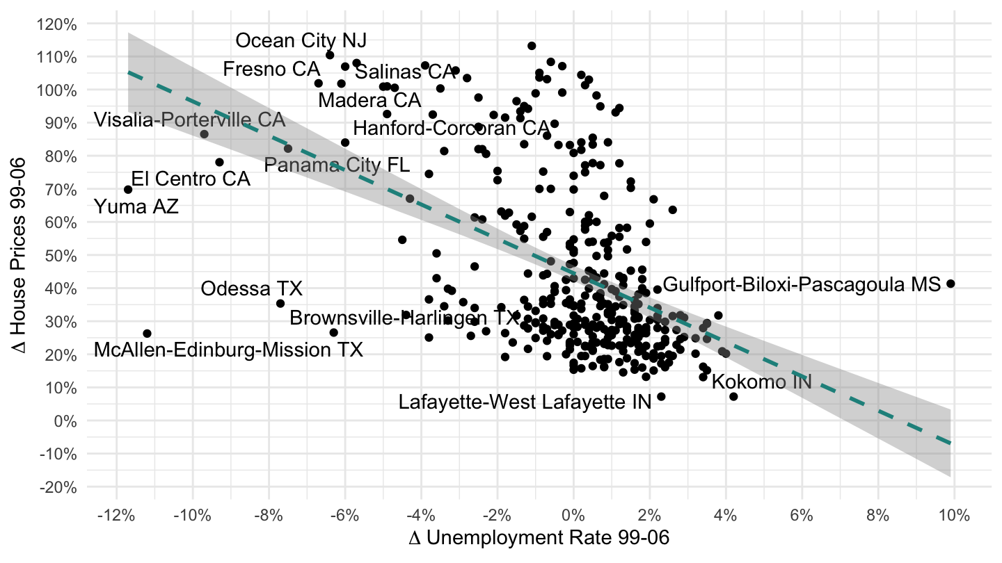
(ref:us-msas-phillips-99-06) U.S. MSAs Phillips curve (99-06)
Code
data2_MSA <- la.data.60.Metro |>
  left_join(la.series, by = "series_id") |>
  left_join(la.measure, by = "measure_code") |>
  select(-area_type_code) |>
  left_join(la.area, by = "area_code") |>
  left_join(la.area_type, by = "area_type_code") |>
  filter(measure_text == "unemployment rate",
         area_type_code == "B") |>
  mutate(fips = area_code |> substr(5, 9) |> as.numeric(),
         value = as.numeric(value),
         month = period |> substr(2, 3),
         date = paste0(year, "-", month, "-01") |> as.Date()) |>
  arrange(fips, date) |>
  filter(date %in% as.Date(paste0(c(1999, 2006), "-01-01"))) |>
  group_by(fips) |>
  mutate(unr_d1 = 0.01*(value - lag(value, 1))) |>
  filter(!is.na(unr_d1)) |>
  select(fips, unr_d1) |>
  left_join(freddie_CBSA |>
              filter(date %in% as.Date(paste0(c(1999, 2006), "-01-01")),
                     variable == "HOUSE_freddie_S") |>
              select(date, fips = cbsa_code, cbsa_name, value) |>
              group_by(fips) |>
              arrange(date) |>
              mutate(HP_d1ln = log(value) - lag(log(value), 1)) |>
              filter(!is.na(HP_d1ln)) |>
              select(fips, cbsa_name, HP_d1ln),
            by = "fips") |>
  na.omit()

data2_MSA |>
  ggplot() + geom_point(aes(unr_d1, HP_d1ln)) + theme_minimal() +
  xlab(expression(Delta~"Unemployment Rate 99-06")) +
  ylab(expression(Delta~"House Prices 99-06")) +
  scale_x_continuous(breaks = 0.01*seq(-20, 20, 2),
                     labels = scales::percent_format(accuracy = 1)) +
  scale_y_continuous(breaks = 0.01*seq(-100, 150, 10),
                     labels = scales::percent_format(accuracy = 1)) +
  geom_text_repel(aes(x = unr_d1, y = HP_d1ln, label = cbsa_name),
            data = data2_MSA |> filter(HP_d1ln<=0.1 | unr_d1 >0.04 | unr_d1 <= -0.06)) +
  stat_smooth(aes(unr_d1, HP_d1ln), linetype = 2,  method = "lm", color = viridis(3)[2])