Labor Force Statistics including the National Unemployment Rate - LN
Data - BLS
Info
Data on employment
| source | dataset | .html | .RData |
|---|---|---|---|
| bls | jt | 2025-08-25 | NA |
| bls | la | 2025-08-25 | NA |
| bls | ln | 2024-11-12 | NA |
| eurostat | nama_10_a10_e | 2025-08-24 | 2025-08-24 |
| eurostat | nama_10_a64_e | 2025-08-24 | 2025-08-24 |
| eurostat | namq_10_a10_e | 2025-05-24 | 2025-08-24 |
| eurostat | une_rt_m | 2025-08-24 | 2025-08-24 |
| oecd | ALFS_EMP | 2024-04-16 | 2025-05-24 |
| oecd | EPL_T | 2025-08-20 | 2023-12-10 |
| oecd | LFS_SEXAGE_I_R | 2024-09-15 | 2024-04-15 |
| oecd | STLABOUR | 2025-01-17 | 2025-01-17 |
LAST_DOWNLOAD
| LAST_DOWNLOAD |
|---|
| 2024-11-12 |
LAST_COMPILE
| LAST_COMPILE |
|---|
| 2025-08-24 |
Last
| date | Nobs |
|---|---|
| 2024-10-01 | 19950 |
ln.activity
Code
ln.data.1.AllData %>%
  left_join(ln.series, by = "series_id") %>%
  left_join(ln.activity, by = "activity_code") %>%
  group_by(activity_code, activity_text) %>%
  summarise(Nobs = n()) %>%
print_table_conditional| activity_code | activity_text | Nobs |
|---|---|---|
| 0 | N/A | 8030958 |
| 3 | Enrolled in School | 156067 |
| 4 | Enrolled in High School | 31158 |
| 5 | Enrolled in College | 31221 |
| 6 | Enrolled in College Full-time | 31182 |
| 7 | Enrolled in College Part-time | 30846 |
| 8 | Not Enrolled | 294052 |
ln.ages
Code
ln.data.1.AllData %>%
  left_join(ln.series, by = "series_id") %>%
  left_join(ln.ages, by = "ages_code") %>%
  group_by(ages_code, ages_text) %>%
  summarise(Nobs = n()) %>%
  print_table_conditional
ln.born
Code
ln.data.1.AllData %>%
  left_join(ln.series, by = "series_id") %>%
  left_join(ln.born, by = "born_code") %>%
  group_by(born_code, born_text) %>%
  summarise(Nobs = n()) %>%
print_table_conditional| born_code | born_text | Nobs |
|---|---|---|
| 0 | N/A | 8532056 |
| 1 | Native born | 36714 |
| 2 | Foreign born | 36714 |
ln.class
Code
ln.data.1.AllData %>%
  left_join(ln.series, by = "series_id") %>%
  left_join(ln.class, by = "class_code") %>%
  group_by(class_code, class_text) %>%
  summarise(Nobs = n()) %>%
print_table_conditional| class_code | class_text | Nobs |
|---|---|---|
| 0 | N/A | 7859879 |
| 1 | Wage and salary workers | 217153 |
| 2 | Private wage and salary workers | 234598 |
| 3 | Government wage and salary workers | 75429 |
| 4 | Federal wage and salary workers | 3723 |
| 5 | State wage and salary workers | 3763 |
| 6 | Local wage and salary workers | 3763 |
| 8 | Self-employed workers, unincorporated | 103766 |
| 9 | Unpaid family workers | 81776 |
| 11 | Nonagriculture government, self employed, and unpaid family worker (3, 8, and 9 above) | 3443 |
| 12 | Self-employed unincorporated, and unpaid family workers (8 and 9) | 3936 |
| 14 | Incorporated self-employed | 2453 |
| 16 | Wage and salary workers, excluding incorporated self employed | 6188 |
| 17 | Private wage and salary workers, excluding incorporated self employed | 4424 |
| 20 | NA | 1190 |
ln.duration
Code
ln.data.1.AllData %>%
  left_join(ln.series, by = "series_id") %>%
  left_join(ln.duration, by = "duration_code") %>%
  group_by(duration_code, duration_text) %>%
  summarise(Nobs = n()) %>%
print_table_conditional| duration_code | duration_text | Nobs |
|---|---|---|
| 0 | N/A | 8115149 |
| 6 | Less than 5 weeks | 98411 |
| 18 | 15 weeks and over | 99467 |
| 31 | 27 weeks and over | 75038 |
| 58 | 52 weeks and over | 28021 |
| 105 | 99 weeks and over | 6286 |
| 106 | 5 to 10 weeks | 2864 |
| 107 | 5 to 14 weeks | 74816 |
| 108 | 11 to 14 weeks | 2848 |
| 109 | 15 to 26 weeks | 74651 |
| 110 | 27 to 51 weeks | 27933 |
ln.education
Code
ln.data.1.AllData %>%
  left_join(ln.series, by = "series_id") %>%
  left_join(ln.education, by = "education_code") %>%
  group_by(education_code, education_text) %>%
  summarise(Nobs = n()) %>%
print_table_conditional| education_code | education_text | Nobs |
|---|---|---|
| 0 | All educational levels | 8240704 |
| 11 | Less than a High School diploma | 65947 |
| 19 | High School graduates, no college | 65975 |
| 20 | Some college or associate degree | 65355 |
| 21 | Some college, no degree | 23864 |
| 25 | Associate degree | 23862 |
| 40 | Bachelor's degree and higher | 77821 |
| 41 | Bachelor's degree only | 20018 |
| 45 | Advanced degree | 21938 |
ln.lfst
Code
ln.data.1.AllData %>%
  left_join(ln.series, by = "series_id") %>%
  left_join(ln.lfst, by = "lfst_code") %>%
  group_by(lfst_code, lfst_text) %>%
  summarise(Nobs = n()) %>%
  print_table_conditional
ln.hour
Code
ln.data.1.AllData %>%
  left_join(ln.series, by = "series_id") %>%
  left_join(ln.hour, by = "hour_code") %>%
  group_by(hour_code, hour_text) %>%
  summarise(Nobs = n()) %>%
print_table_conditional| hour_code | hour_text | Nobs |
|---|---|---|
| 0 | N/A | 8234248 |
| 1 | 1 to 34 hours | 207416 |
| 2 | 1 to 4 hours | 7695 |
| 6 | 5 to 14 hours | 7695 |
| 10 | 15 to 29 hours | 6979 |
| 14 | 30 to 34 hours | 8411 |
| 16 | 35 hours and over | 93314 |
| 17 | 35 to 39 hours | 6979 |
| 20 | 40 hours | 6979 |
| 21 | 41 hours and over | 4831 |
| 23 | 41 to 48 hours | 6979 |
| 27 | 49 to 59 hours | 6979 |
| 29 | 60 hours and over | 6979 |
ln.indy
Code
ln.data.1.AllData %>%
  left_join(ln.series, by = "series_id") %>%
  left_join(ln.indy, by = "indy_code") %>%
  group_by(indy_code, indy_text) %>%
  summarise(Nobs = n()) %>%
  print_table_conditional
ln.occupation
Code
ln.data.1.AllData %>%
  left_join(ln.series, by = "series_id") %>%
  left_join(ln.occupation, by = "occupation_code") %>%
  group_by(occupation_code, occupation_text) %>%
  summarise(Nobs = n()) %>%
  print_table_conditional
ln.orig
Code
ln.data.1.AllData %>%
  left_join(ln.series, by = "series_id") %>%
  left_join(ln.orig, by = "orig_code") %>%
  group_by(orig_code, orig_text) %>%
  summarise(Nobs = n()) %>%
print_table_conditional| orig_code | orig_text | Nobs |
|---|---|---|
| 0 | All Origins | 7656155 |
| 1 | Hispanic or Latino | 771886 |
| 2 | Mexican | 40737 |
| 6 | Puerto Rican | 39578 |
| 7 | Cuban | 39088 |
| 10 | Non-Hispanic | 28440 |
| 15 | Central or South American | 4392 |
| 20 | Central American | 4392 |
| 21 | Salvadoran | 1624 |
| 25 | Other Central American (excludes Salvadoran) | 4392 |
| 30 | South American | 4392 |
| 40 | Other Hispanic or Latino | 4392 |
| 41 | Dominican | 1624 |
| 45 | Other Hispanic or Latino (excludes Dominican) | 4392 |
ln.race
Code
ln.data.1.AllData %>%
  left_join(ln.series, by = "series_id") %>%
  left_join(ln.race, by = "race_code") %>%
  group_by(race_code, race_text) %>%
  summarise(Nobs = n()) %>%
print_table_conditional| race_code | race_text | Nobs |
|---|---|---|
| 0 | All Races | 5720368 |
| 1 | White | 1286531 |
| 3 | Black or African American | 1044875 |
| 4 | Asian | 532298 |
| 5 | American Indian or Alaska Native | 3722 |
| 6 | Native Hawaiian or Other Pacific Islander | 3314 |
| 7 | Two or more races | 3176 |
| 10 | Asian Indian | 1600 |
| 15 | Chinese | 1600 |
| 25 | Filipino | 1600 |
| 26 | Japanese | 1600 |
| 27 | Korean | 1600 |
| 28 | Vietnamese | 1600 |
| 30 | Other Asian | 1600 |
ln.seasonal
Code
ln.data.1.AllData %>%
  left_join(ln.series, by = "series_id") %>%
  rename(seasonal_code = seasonal) %>%
  left_join(ln.seasonal, by = "seasonal_code") %>%
  group_by(seasonal_code, seasonal_text) %>%
  summarise(Nobs = n()) %>%
print_table_conditional| seasonal_code | seasonal_text | Nobs |
|---|---|---|
| S | Seasonally Adjusted | 581747 |
| U | Not Seasonally Adjusted | 8023737 |
ln.sexs
Code
ln.data.1.AllData %>%
  left_join(ln.series, by = "series_id") %>%
  left_join(ln.sexs, by = "sexs_code") %>%
  group_by(sexs_code, sexs_text) %>%
  summarise(Nobs = n()) %>%
print_table_conditional| sexs_code | sexs_text | Nobs |
|---|---|---|
| 0 | Both Sexes | 3985561 |
| 1 | Men | 2324247 |
| 2 | Women | 2295676 |
ln.vets
Code
ln.data.1.AllData %>%
  left_join(ln.series, by = "series_id") %>%
  left_join(ln.vets, by = "vets_code") %>%
  group_by(vets_code, vets_text) %>%
  summarise(Nobs = n()) %>%
print_table_conditional| vets_code | vets_text | Nobs |
|---|---|---|
| 0 | N/A | 8056827 |
| 1 | Veteran | 144288 |
| 3 | World War II or Korean War or Vietnam Era | 39272 |
| 9 | Gulf War Era | 63975 |
| 12 | Veterans who served in Gulf War Era 2 (whether or not they served in Era 1) | 57611 |
| 13 | Veterans who served in Gulf War Era 1 but not Gulf War Era 2 | 50973 |
| 16 | Other Service Periods (may include peacetime) | 48648 |
| 25 | Nonveteran | 143890 |
Longest Series
Code
ln.series %>%
  arrange(begin_year) %>%
  head(100) %>%
  select(series_id, series_title, begin_year, end_year) %>%
  {if (is_html_output()) datatable(., filter = 'top', rownames = F) else .}
Employment / Population Ratio
All Series - lfst_code = 23
Code
ln.data.1.AllData %>%
  left_join(ln.series, by = "series_id") %>%
  filter(lfst_code == 23) %>%
  group_by(series_id, series_title) %>%
  summarise(Nobs = n()) %>%
  print_table_conditional
Men, Women, All
All
Code
ln.data.1.AllData %>%
  left_join(ln.series, by = "series_id") %>%
  #filter(series_id %in% c("LNS12300001", "LNS12300000", "LNS12300002")) %>%
  left_join(ln.sexs, by = "sexs_code") %>%
  filter(lfst_code == 23,
         orig_code == 0,
         born_code == 0,
         mari_code == 0,
         race_code == 0,
         seasonal == "S",
         ages_code == 0,
         activity_code == 0,
         duration_code == 0) %>%
  month_to_date() %>%
  mutate(value = as.numeric(value)) %>%
  ggplot(.) + theme_minimal() + xlab("") +
  ylab("Employment / Population Ratio") +
  geom_line(aes(x = date, y = value/100, color = sexs_text)) +
  geom_rect(data = nber_recessions %>%
              filter(Trough >= as.Date("1947-01-01")),
            aes(xmin = Peak, xmax = Trough, ymin = -Inf, ymax = +Inf),
            fill = 'grey', alpha = 0.5) +
  scale_x_date(breaks = seq(1910, 2100, 5) %>% paste0("-01-01") %>% as.Date,
               labels = date_format("%Y")) +
  scale_y_continuous(breaks = 0.01*c(seq(0, 100, 10), seq(100, 500, 50)),
                     labels = percent_format(accuracy = 1, prefix = "")) +
  scale_color_manual(values = c("black", "darkblue", "purple")) +
  theme(legend.position = c(0.8, 0.2),
        legend.title = element_blank())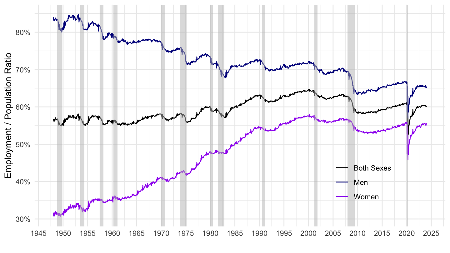
1980-
Code
ln.data.1.AllData %>%
  left_join(ln.series, by = "series_id") %>%
  #filter(series_id %in% c("LNS12300001", "LNS12300000", "LNS12300002")) %>%
  left_join(ln.sexs, by = "sexs_code") %>%
  filter(lfst_code == 23,
         orig_code == 0,
         born_code == 0,
         mari_code == 0,
         race_code == 0,
         seasonal == "S",
         ages_code == 0,
         activity_code == 0,
         duration_code == 0) %>%
  month_to_date() %>%
  arrange(desc(date)) %>%
  filter(date >= as.Date("1980-01-01")) %>%
  mutate(value = as.numeric(value)) %>%
  ggplot(.) + theme_minimal() + xlab("") +
  ylab("Employment / Population Ratio") +
  geom_line(aes(x = date, y = value/100, color = sexs_text)) +
  geom_rect(data = nber_recessions %>%
              filter(Trough >= as.Date("1980-01-01")),
            aes(xmin = Peak, xmax = Trough, ymin = -Inf, ymax = +Inf),
            fill = 'grey', alpha = 0.5) +
  scale_x_date(breaks = seq(1910, 2100, 5) %>% paste0("-01-01") %>% as.Date,
               labels = date_format("%Y")) +
  scale_y_continuous(breaks = 0.01*c(seq(0, 100, 5), seq(100, 500, 50)),
                     labels = percent_format(accuracy = 1, prefix = "")) +
  scale_color_manual(values = c("black", "darkblue", "purple")) +
  theme(legend.position = c(0.8, 0.2),
        legend.title = element_blank())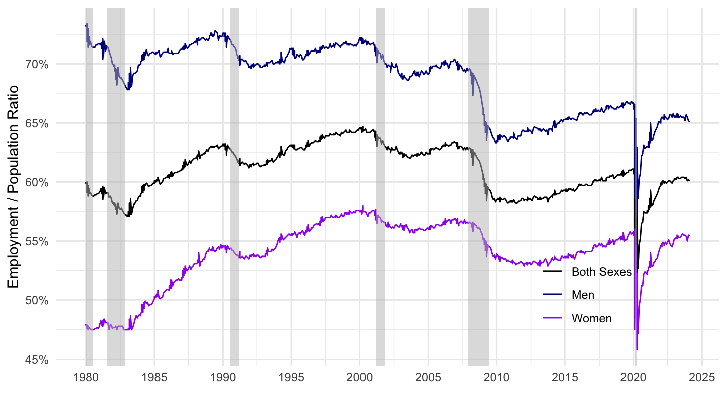
Veterans, Non Veterans
Code
ln.series %>%
  filter(lfst_code == 23,
         sexs_code == 1,
         race_code == 0,
         seasonal == "U",
         ages_code == 28,
         orig_code == 0,
         born_code == 0,
         education_code == 0,
         periodicity_code == "M") %>%
  left_join(ln.data.1.AllData, by = "series_id") %>%
  #filter(series_id %in% c("LNS12300001", "LNS12300049", "LNS12300061")) %>%
  left_join(ln.vets, by = "vets_code") %>%
  month_to_date() %>%
  mutate(value = as.numeric(value)) %>%
  ggplot(.) + theme_minimal() + xlab("") + ylab("Men Employment / Population Ratio") +
  geom_line(aes(x = date, y = value/100, color = vets_text)) +
  geom_rect(data = nber_recessions %>%
              filter(Trough >= as.Date("1947-01-01")),
            aes(xmin = Peak, xmax = Trough, ymin = -Inf, ymax = +Inf),
            fill = 'grey', alpha = 0.5) +

  theme(legend.position = c(0.2, 0.2),
        legend.title = element_blank()) +
  scale_x_date(breaks = seq(1910, 2100, 5) %>% paste0("-01-01") %>% as.Date,
               labels = date_format("%Y")) +
  scale_y_continuous(breaks = 0.01*c(seq(0, 100, 5), seq(100, 500, 50)),
                     labels = percent_format(accuracy = 1, prefix = ""))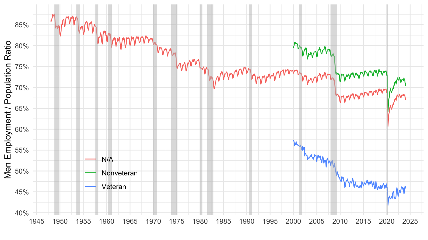
By age, Men
Seasonal
All
Code
ln.series %>%
  filter(lfst_code == 23,
         sexs_code == 1,
         race_code == 0,
         mari_code == 0,
         seasonal == "S",
         ages_code %in% c(0, 28, 33, 22),
         periodicity_code == "M") %>%
  left_join(ln.data.1.AllData, by = "series_id") %>%
  #filter(series_id %in% c("LNS12300001", "LNS12300049", "LNS12300061")) %>%
  left_join(ln.ages, by = "ages_code") %>%
  month_to_date() %>%
  mutate(value = as.numeric(value)) %>%
  ggplot(.) + theme_minimal() + xlab("") + ylab("Men Employment / Population Ratio") +
  geom_line(aes(x = date, y = value/100, color = ages_text)) +
  geom_rect(data = nber_recessions %>%
              filter(Trough >= as.Date("1947-01-01")),
            aes(xmin = Peak, xmax = Trough, ymin = -Inf, ymax = +Inf),
            fill = 'grey', alpha = 0.5) +
  theme(legend.position = c(0.2, 0.2),
        legend.title = element_blank()) +
  scale_x_date(breaks = seq(1910, 2100, 5) %>% paste0("-01-01") %>% as.Date,
               labels = date_format("%Y")) +
  scale_y_continuous(breaks = 0.01*c(seq(0, 100, 5), seq(100, 500, 50)),
                     labels = percent_format(accuracy = 1, prefix = ""))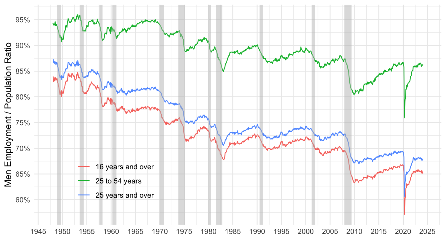
1980-
Code
ln.series %>%
  filter(lfst_code == 23,
         sexs_code == 1,
         race_code == 0,
         mari_code == 0,
         seasonal == "S",
         ages_code %in% c(0, 28, 33, 22),
         periodicity_code == "M") %>%
  left_join(ln.data.1.AllData, by = "series_id") %>%
  #filter(series_id %in% c("LNS12300001", "LNS12300049", "LNS12300061")) %>%
  left_join(ln.ages, by = "ages_code") %>%
  month_to_date() %>%
  filter(date >= as.Date("1980-01-01")) %>%
  mutate(value = as.numeric(value)) %>%
  ggplot(.) + theme_minimal() + xlab("") + ylab("Men Employment / Population Ratio") +
  geom_line(aes(x = date, y = value/100, color = ages_text)) +
  geom_rect(data = nber_recessions %>%
              filter(Trough >= as.Date("1980-01-01")),
            aes(xmin = Peak, xmax = Trough, ymin = -Inf, ymax = +Inf),
            fill = 'grey', alpha = 0.5) +
  theme(legend.position = c(0.2, 0.2),
        legend.title = element_blank()) +
  scale_x_date(breaks = seq(1910, 2100, 5) %>% paste0("-01-01") %>% as.Date,
               labels = date_format("%Y")) +
  scale_y_continuous(breaks = 0.01*c(seq(0, 100, 5), seq(100, 500, 50)),
                     labels = percent_format(accuracy = 1, prefix = ""))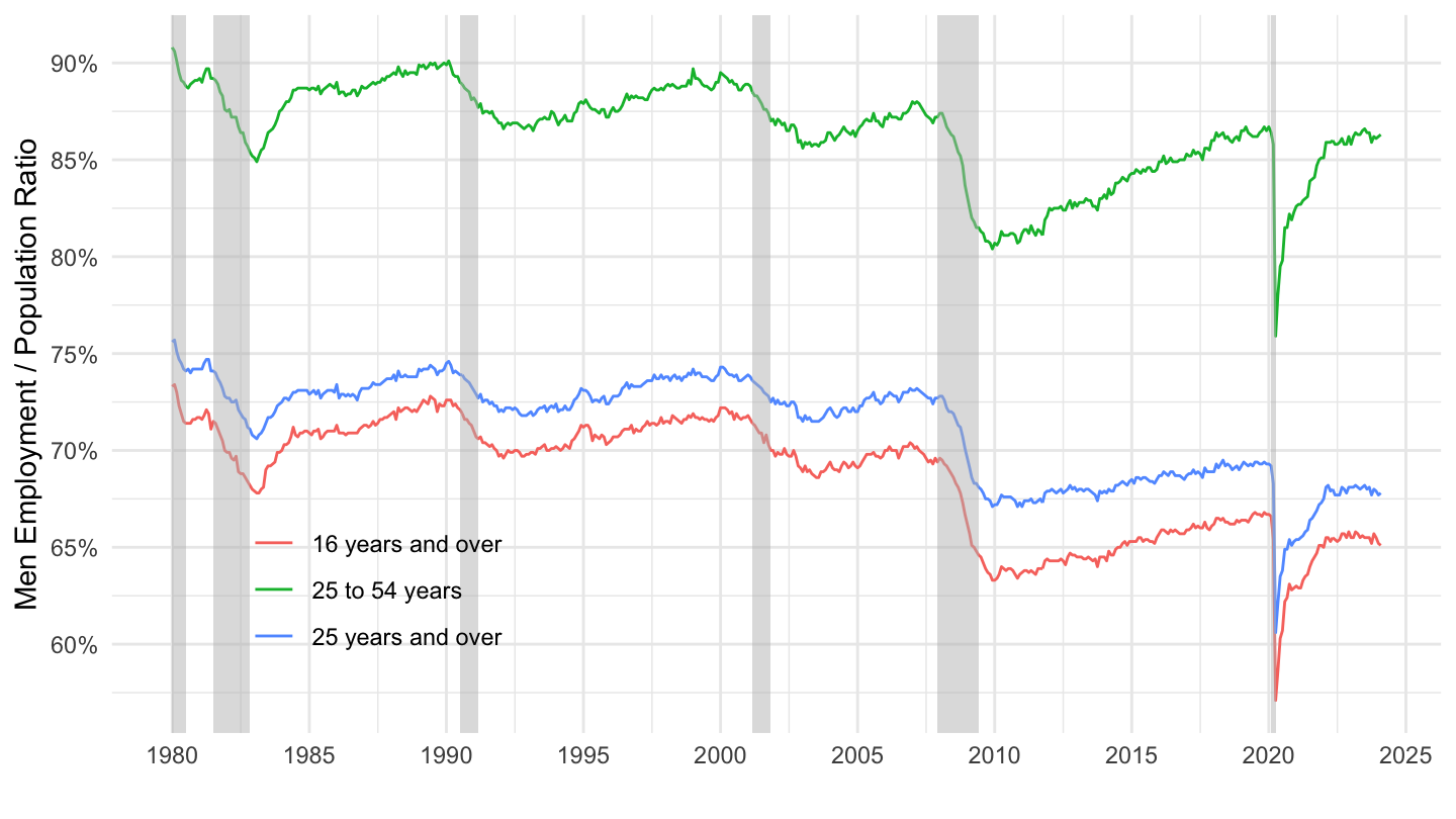
Seasonal
Code
ln.series %>%
  filter(lfst_code == 23,
         sexs_code == 1,
         race_code == 0,
         seasonal == "S",
         ages_code %in% c(33),
         periodicity_code == "M") %>%
  left_join(ln.data.1.AllData, by = "series_id") %>%
  #filter(series_id %in% c("LNS12300001", "LNS12300049", "LNS12300061")) %>%
  left_join(ln.ages, by = "ages_code") %>%
  month_to_date() %>%
  mutate(value = as.numeric(value)) %>%
  ggplot(.) + theme_minimal() + xlab("") + ylab("25-54 Men Employment / Population Ratio") +
  geom_line(aes(x = date, y = value/100)) +
  geom_rect(data = nber_recessions %>%
              filter(Trough >= as.Date("1947-01-01")),
            aes(xmin = Peak, xmax = Trough, ymin = -Inf, ymax = +Inf),
            fill = 'grey', alpha = 0.5) +
  theme(legend.position = c(0.2, 0.2),
        legend.title = element_blank()) +
  scale_x_date(breaks = seq(1910, 2100, 5) %>% paste0("-01-01") %>% as.Date,
               labels = date_format("%Y")) +
  scale_y_continuous(breaks = 0.01*c(seq(0, 100, 5), seq(100, 500, 50)),
                     labels = percent_format(accuracy = 1, prefix = ""))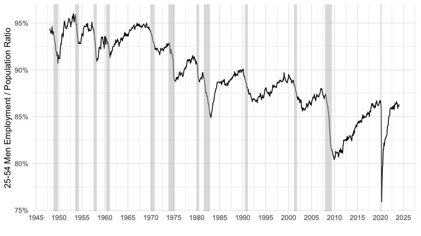
Unseasonal
Code
ln.series %>%
  filter(lfst_code == 23,
         sexs_code == 1,
         race_code == 0,
         seasonal == "U",
         ages_code %in% c(0, 28, 33),
         orig_code == 0,
         mari_code == 0,
         born_code == 0,
         vets_code == 0,
         education_code == 0,
         periodicity_code == "M") %>%
  left_join(ln.data.1.AllData, by = "series_id") %>%
  #filter(series_id %in% c("LNS12300001", "LNS12300049", "LNS12300061")) %>%
  left_join(ln.ages, by = "ages_code") %>%
  month_to_date() %>%
  arrange(desc(date)) %>%
  mutate(value = as.numeric(value)) %>%
  ggplot(.) + theme_minimal() + xlab("") + ylab("Men Employment / Population Ratio") +
  geom_line(aes(x = date, y = value/100, color = ages_text)) +
  geom_rect(data = nber_recessions %>%
              filter(Trough >= as.Date("1947-01-01")),
            aes(xmin = Peak, xmax = Trough, ymin = -Inf, ymax = +Inf),
            fill = 'grey', alpha = 0.5) +
  theme(legend.position = c(0.2, 0.2),
        legend.title = element_blank()) +
  scale_x_date(breaks = seq(1910, 2100, 5) %>% paste0("-01-01") %>% as.Date,
               labels = date_format("%Y")) +
  scale_y_continuous(breaks = 0.01*c(seq(0, 100, 5), seq(100, 500, 50)),
                     labels = percent_format(accuracy = 1, prefix = ""))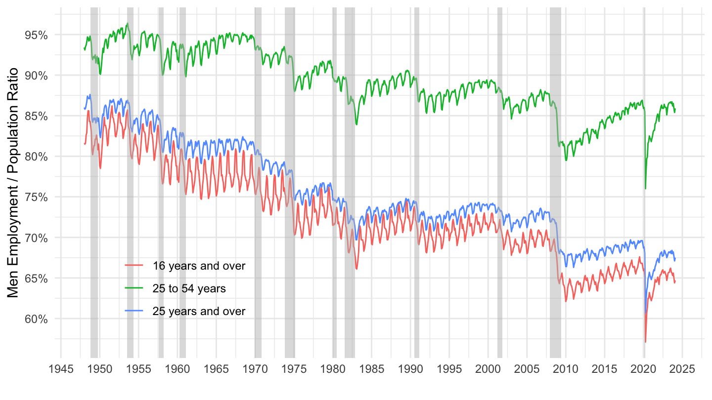
Men, Women
1994-
Code
ln.series %>%
  filter(lfst_code == 23,
         race_code == 0,
         seasonal == "S",
         ages_code %in% c(33),
         periodicity_code == "M") %>%
  left_join(ln.data.1.AllData, by = "series_id") %>%
  #filter(series_id %in% c("LNS12300001", "LNS12300049", "LNS12300061")) %>%
  left_join(ln.sexs, by = "sexs_code") %>%
  month_to_date() %>%
  filter(date >= as.Date("1994-01-01")) %>%
  mutate(value = as.numeric(value)) %>%
  ggplot(.) + theme_minimal() + xlab("") + ylab("25-54 Men Employment / Population Ratio") +
  geom_line(aes(x = date, y = value/100, color = sexs_text)) +
  geom_rect(data = nber_recessions %>%
              filter(Trough >= as.Date("1994-01-01")),
            aes(xmin = Peak, xmax = Trough, ymin = -Inf, ymax = +Inf),
            fill = 'grey', alpha = 0.5) +
  scale_color_manual(values = c("black", "darkblue", "purple")) +
  theme(legend.position = c(0.8, 0.2),
        legend.title = element_blank()) +
  scale_x_date(breaks = seq(1910, 2100, 2) %>% paste0("-01-01") %>% as.Date,
               labels = date_format("%Y")) +
  scale_y_continuous(breaks = 0.01*c(seq(0, 100, 5), seq(100, 500, 50)),
                     labels = percent_format(accuracy = 1, prefix = ""))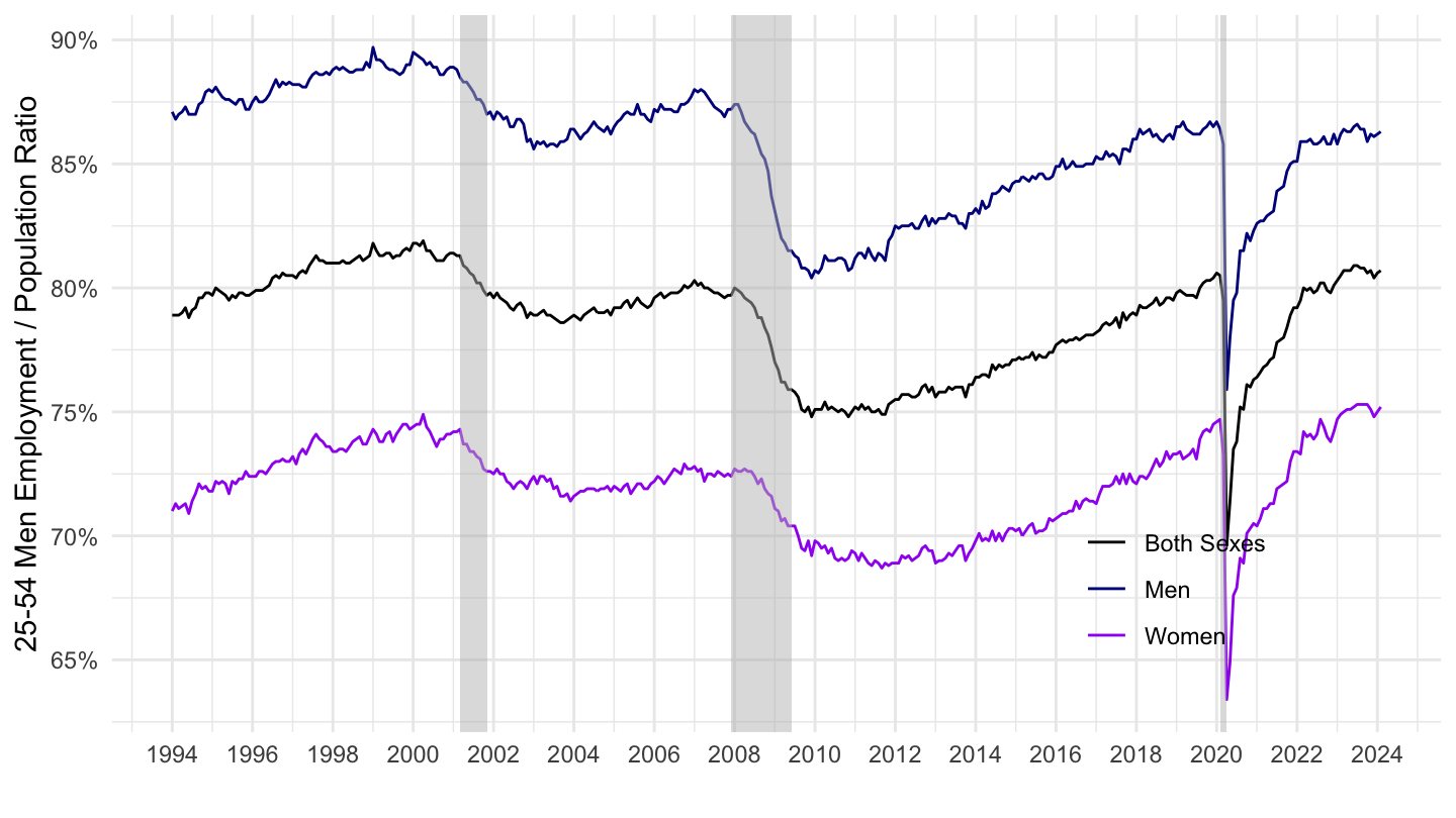
All
Code
ln.series %>%
  filter(lfst_code == 23,
         race_code == 0,
         seasonal == "S",
         ages_code %in% c(33),
         periodicity_code == "M") %>%
  left_join(ln.data.1.AllData, by = "series_id") %>%
  #filter(series_id %in% c("LNS12300001", "LNS12300049", "LNS12300061")) %>%
  left_join(ln.sexs, by = "sexs_code") %>%
  month_to_date() %>%
  mutate(value = as.numeric(value)) %>%
  ggplot(.) + theme_minimal() + xlab("") + ylab("25-54 Men Employment / Population Ratio") +
  geom_line(aes(x = date, y = value/100, color = sexs_text)) +
  geom_rect(data = nber_recessions %>%
              filter(Trough >= as.Date("1947-01-01")),
            aes(xmin = Peak, xmax = Trough, ymin = -Inf, ymax = +Inf),
            fill = 'grey', alpha = 0.5) +
  scale_color_manual(values = c("black", "darkblue", "purple")) +
  theme(legend.position = c(0.8, 0.2),
        legend.title = element_blank()) +
  scale_x_date(breaks = seq(1910, 2100, 2) %>% paste0("-01-01") %>% as.Date,
               labels = date_format("%Y")) +
  scale_y_continuous(breaks = 0.01*c(seq(0, 100, 5), seq(100, 500, 50)),
                     labels = percent_format(accuracy = 1, prefix = ""))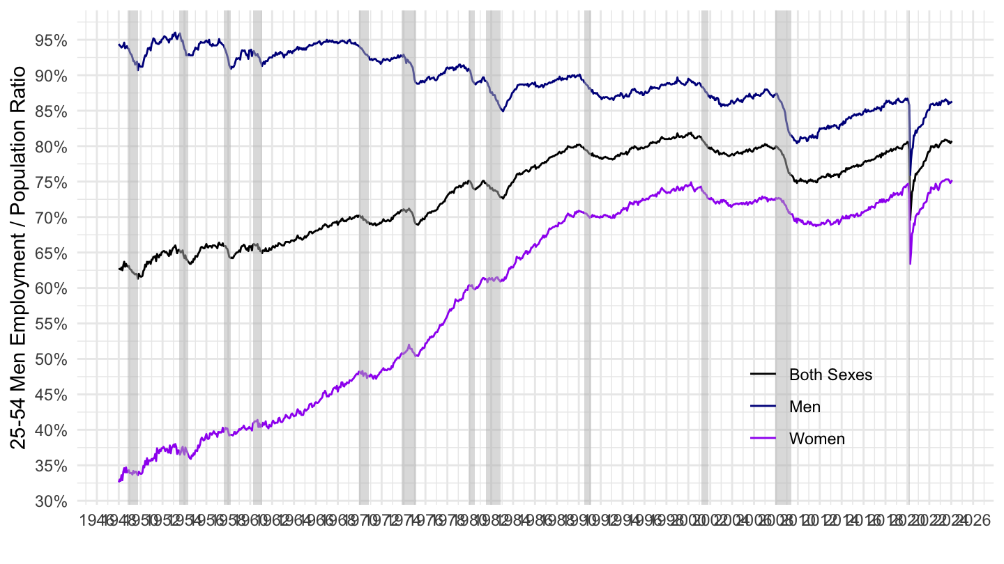
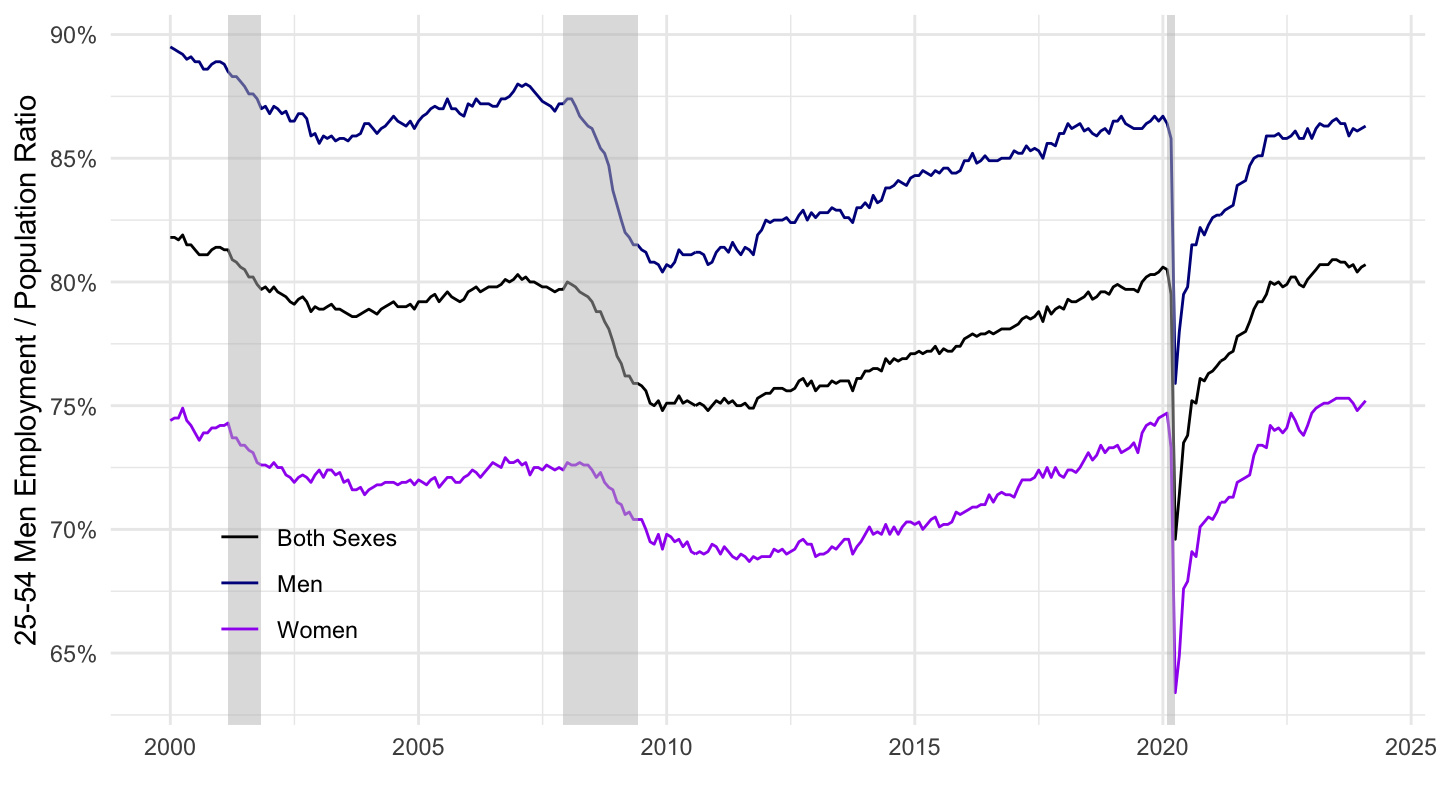
2009-
Code
ln.series %>%
  filter(lfst_code == 23,
         race_code == 0,
         seasonal == "S",
         ages_code %in% c(33),
         periodicity_code == "M") %>%
  left_join(ln.data.1.AllData, by = "series_id") %>%
  #filter(series_id %in% c("LNS12300001", "LNS12300049", "LNS12300061")) %>%
  left_join(ln.sexs, by = "sexs_code") %>%
  month_to_date() %>%
  filter(date >= as.Date("2000-01-01")) %>%
  mutate(value = as.numeric(value)) %>%
  ggplot(.) + theme_minimal() + xlab("") + ylab("25-54 Men Employment / Population Ratio") +
  geom_line(aes(x = date, y = value/100, color = sexs_text)) +
  geom_rect(data = nber_recessions %>%
              filter(Trough >= as.Date("2000-01-01")),
            aes(xmin = Peak, xmax = Trough, ymin = -Inf, ymax = +Inf),
            fill = 'grey', alpha = 0.5) +
  scale_color_manual(values = c("black", "darkblue", "purple")) +
  theme(legend.position = c(0.15, 0.2),
        legend.title = element_blank()) +
  scale_x_date(breaks = seq(1910, 2100, 5) %>% paste0("-01-01") %>% as.Date,
               labels = date_format("%Y")) +
  scale_y_continuous(breaks = 0.01*c(seq(0, 100, 5), seq(100, 500, 50)),
                     labels = percent_format(accuracy = 1, prefix = ""))