World Bank Commodity Price Data (The Pink Sheet)

Data - WB

Author

Info

source	dataset	.html	.RData
wb	CMO	2024-12-21	2024-12-22

Data on energy

source	dataset	.html	.RData
ec	WOB	2024-12-22	2024-08-25
eurostat	ei_isen_m	2024-11-23	2024-10-09
eurostat	nrg_bal_c	2023-12-31	2024-10-08
eurostat	nrg_pc_202	2024-12-21	2024-12-21
eurostat	nrg_pc_203	2023-06-11	2024-10-08
eurostat	nrg_pc_203_c	2024-11-22	2024-10-08
eurostat	nrg_pc_203_h	2024-11-22	2024-12-22
eurostat	nrg_pc_203_v	2024-11-22	2024-10-08
eurostat	nrg_pc_204	2024-12-21	2024-12-22
eurostat	nrg_pc_205	2023-06-11	2024-10-08
fred	energy	2024-12-22	2024-12-22
iea	world_energy_balances_highlights_2022	2024-06-20	2023-04-24
wb	CMO	2024-12-21	2024-12-22
wdi	EG.GDP.PUSE.KO.PP.KD	2024-09-18	2024-09-18
wdi	EG.USE.PCAP.KG.OE	2024-09-18	2024-09-18
yahoo	energy	2024-12-22	2024-12-22

Data on industry

source	dataset	.html	.RData
ec	INDUSTRY	2024-09-15	2023-10-01
eurostat	ei_isin_m	2024-11-23	2024-10-09
eurostat	htec_trd_group4	2024-11-23	2024-10-08
eurostat	nama_10_a64	2024-12-21	2024-12-21
eurostat	nama_10_a64_e	2024-12-21	2024-12-21
eurostat	namq_10_a10_e	2024-12-21	2024-12-21
eurostat	road_eqr_carmot	2024-11-22	2024-10-08
eurostat	sts_inpp_m	2024-06-24	2024-12-21
eurostat	sts_inppd_m	2024-12-21	2024-12-21
eurostat	sts_inpr_m	2024-11-22	2024-10-08
eurostat	sts_intvnd_m	2024-12-21	2024-12-21
fred	industry	2024-12-22	2024-12-22
oecd	ALFS_EMP	2024-04-16	2024-12-21
oecd	BERD_MA_SOF	2024-04-16	2023-09-09
oecd	GBARD_NABS2007	2024-04-16	2023-11-22
oecd	MEI_REAL	2024-05-12	2024-12-21
oecd	MSTI_PUB	2024-09-15	2024-12-21
oecd	SNA_TABLE4	2024-09-15	2024-12-16
wdi	NV.IND.EMPL.KD	2024-01-06	2024-09-18
wdi	NV.IND.MANF.CD	2024-12-21	2024-12-21
wdi	NV.IND.MANF.ZS	2024-12-21	2024-12-21
wdi	NV.IND.TOTL.KD	2024-01-06	2024-09-18
wdi	NV.IND.TOTL.ZS	2024-12-21	2024-12-21
wdi	SL.IND.EMPL.ZS	2024-12-21	2024-12-21
wdi	TX.VAL.MRCH.CD.WT	2024-01-06	2024-09-18

LAST_COMPILE

LAST_COMPILE
2024-12-22

Last

date	Nobs
2024-11-01	68

variable

Natural Gas: Europe and US

Nominal prices

Linear

Code

plot_linear <- CMO %>%
  filter(Variable %in% c("Natural gas, US", "Natural gas, Europe")) %>%
  ggplot + geom_line(aes(x = date, y = value, color = Variable)) +
  labs(x = "", y = "Price of natural gas (Current $/mmbtu)") + theme_minimal() +
  scale_x_date(breaks = seq(1920, 2025, 10) %>% paste0("-01-01") %>% as.Date,
               labels = date_format("%Y")) +
  scale_color_manual(values = viridis(3)[1:2]) +
  theme(legend.position = c(0.4, 0.8),
        legend.title = element_blank()) +
  scale_y_continuous(breaks = seq(-20, 400, 10),
                     labels = dollar_format(a = 1))

plot_linear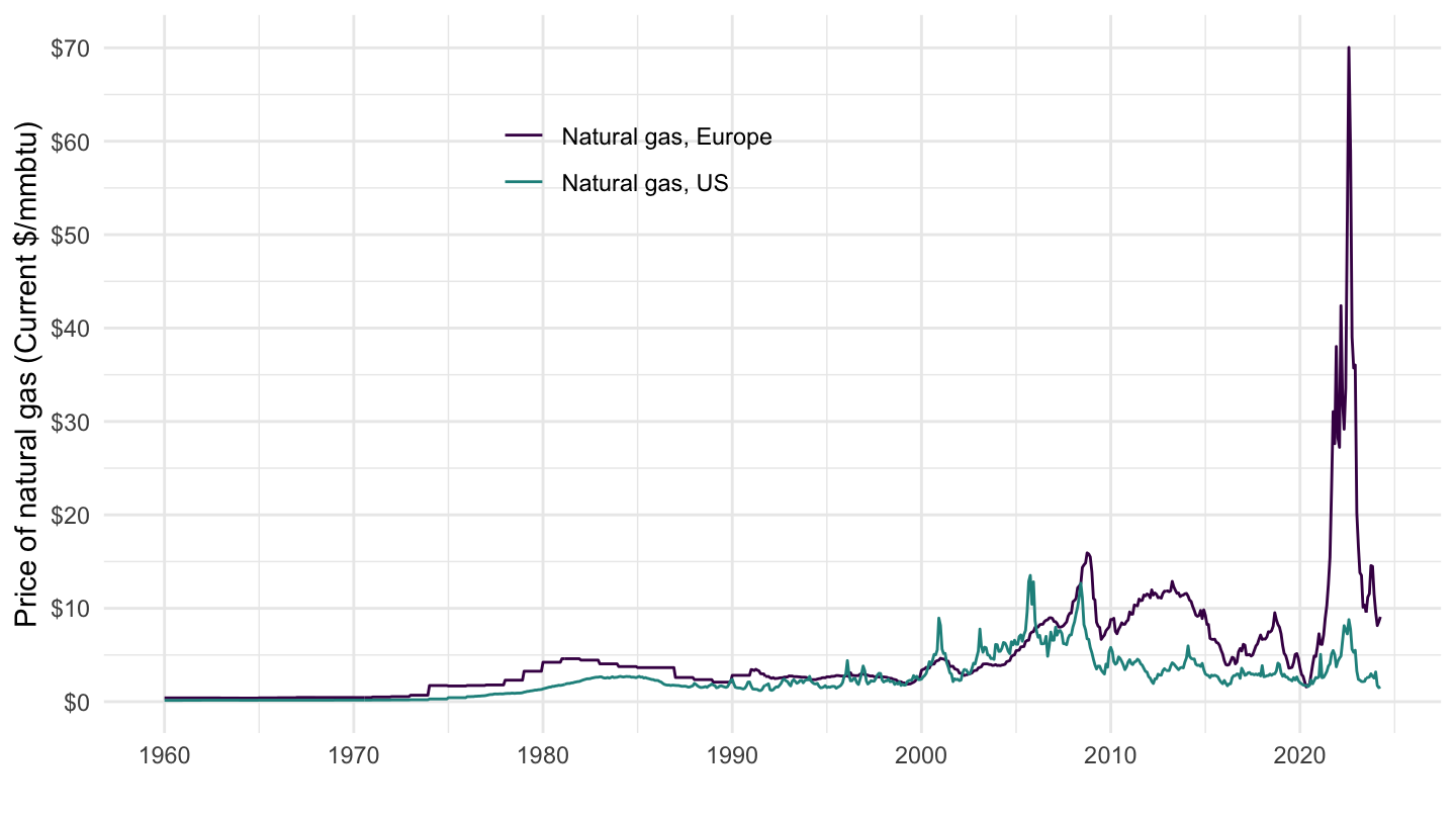

Log

All

Code

plot_log <- CMO %>%
  filter(Variable %in% c("Natural gas, US", "Natural gas, Europe")) %>%
  ggplot + geom_line(aes(x = date, y = value, color = Variable)) +
  labs(x = "", y = "Price of natural gas (Current $/mmbtu)") + theme_minimal() +
  scale_x_date(breaks = seq(1920, 2025, 10) %>% paste0("-01-01") %>% as.Date,
               labels = date_format("%Y")) +
  scale_color_manual(values = viridis(3)[1:2]) +
  theme(legend.position = c(0.4, 0.8),
        legend.title = element_blank()) +
  scale_y_log10(breaks = c(0.1, 0.2, 0.3, 0.5, 0.8, 1, 2, 3, 4, 5, 8, 10, 15, 20, 30, 40, 50),
                     labels = dollar_format(a = .1))

plot_log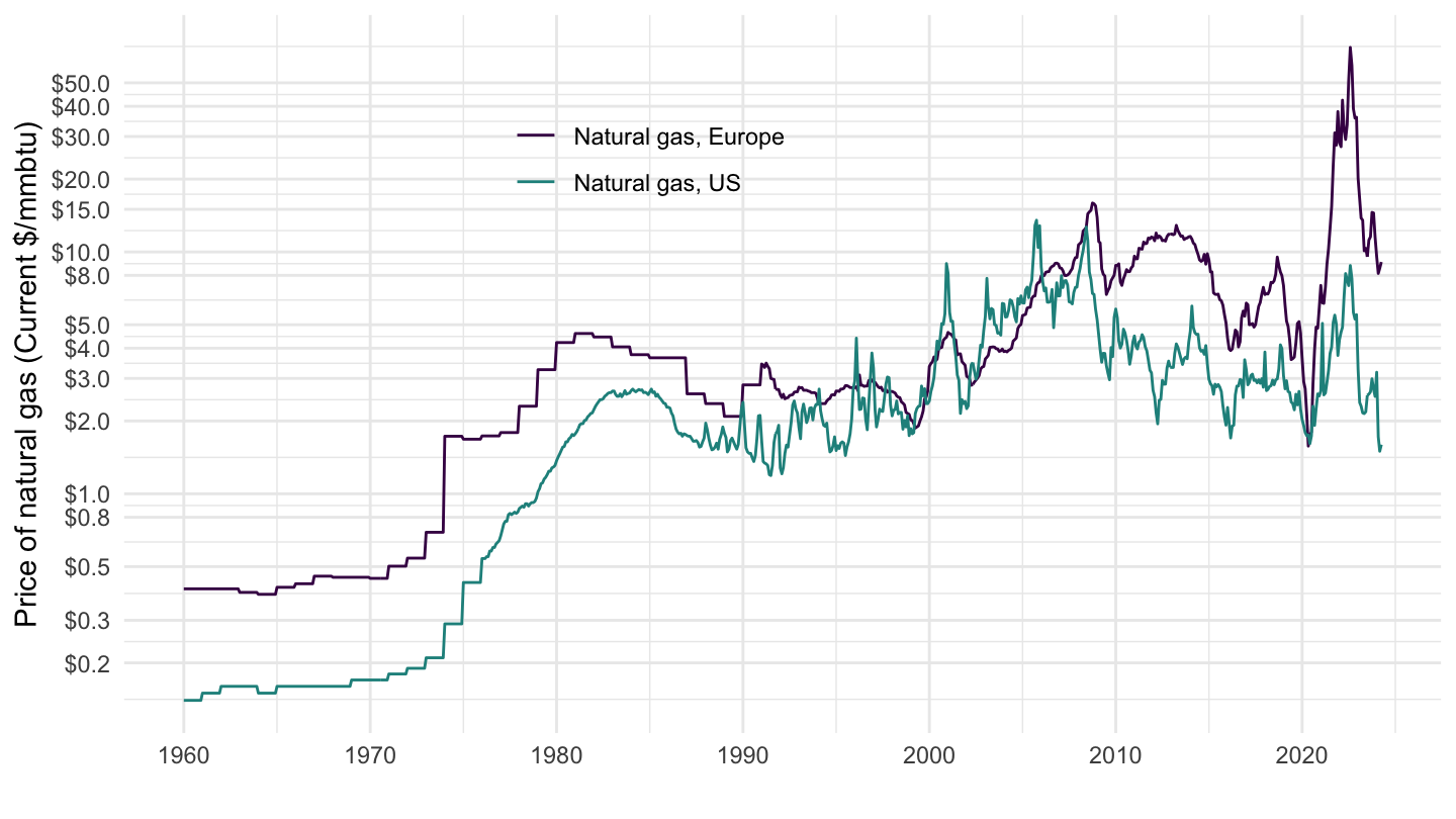

1990-

Code

CMO %>%
  filter(Variable %in% c("Natural gas, US", "Natural gas, Europe")) %>%
  filter(date >= as.Date("1990-01-01")) %>%
  ggplot + geom_line(aes(x = date, y = value, color = Variable)) +
  labs(x = "", y = "Price of natural gas (Current $/mmbtu)") + theme_minimal() +
  scale_x_date(breaks = seq(1920, 2025, 5) %>% paste0("-01-01") %>% as.Date,
               labels = date_format("%Y")) +
  scale_color_manual(values = viridis(3)[1:2]) +
  theme(legend.position = c(0.4, 0.8),
        legend.title = element_blank()) +
  scale_y_log10(breaks = c(0.1, 0.2, 0.3, 0.5, 0.8, 1, 2, 3, 4, 5, 8, 10, 15, 20, 30, 40, 50, 80, 100),
                     labels = dollar_format(a = 1))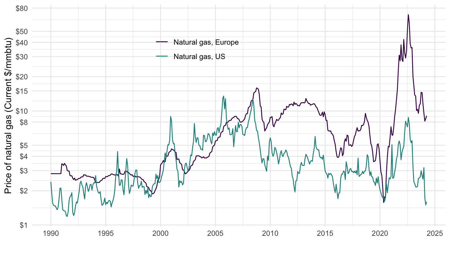

2000-

Code

CMO %>%
  filter(Variable %in% c("Natural gas, US", "Natural gas, Europe")) %>%
  filter(date >= as.Date("2000-01-01")) %>%
  ggplot + geom_line(aes(x = date, y = value, color = Variable)) +
  labs(x = "", y = "Price of natural gas (Current $/mmbtu)") + theme_minimal() +
  scale_x_date(breaks = seq(1920, 2025, 2) %>% paste0("-01-01") %>% as.Date,
               labels = scales::date_format("%Y")) +
  scale_color_manual(values = viridis(3)[1:2]) +
  theme(legend.position = c(0.4, 0.8),
        legend.title = element_blank()) +
  scale_y_log10(breaks = c(0.1, 0.2, 0.3, 0.5, 0.8, 1, 2, 3, 4, 5, 8, 10, 15, 20, 30, 40, 50, 80, 100),
                     labels = dollar_format(a = 1))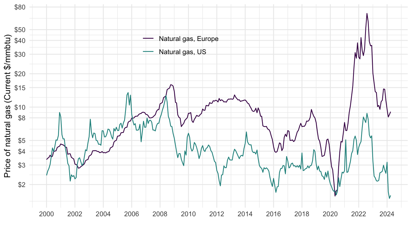

Bind

Code

ggpubr::ggarrange(plot_linear + ggtitle("Linear Scale"), plot_log  + ggtitle("Log Scale"), common.legend = T)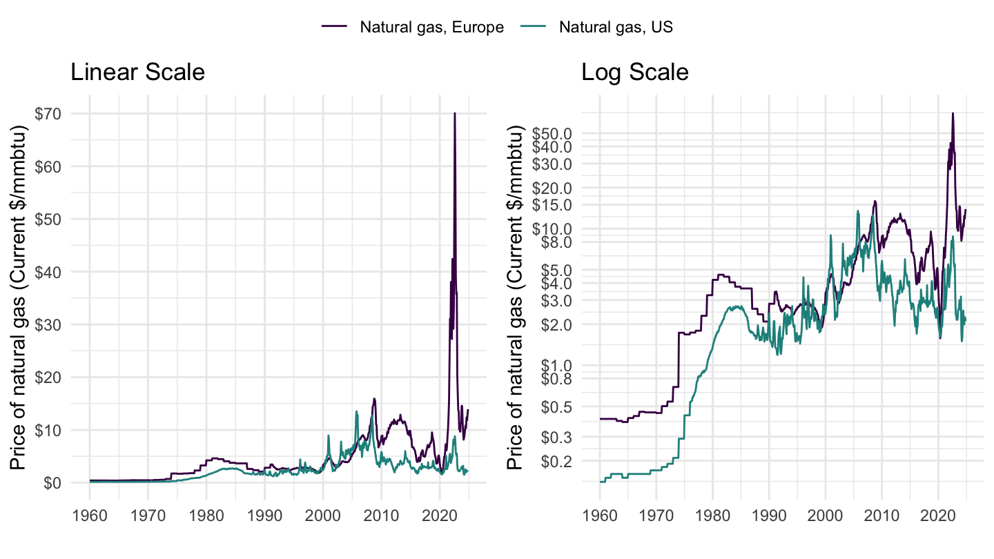

Real prices

Linear

Code

plot_linear <- CMO %>%
  filter(Variable %in% c("Natural gas, US", "Natural gas, Europe")) %>%
  left_join(CPIAUCSL, by = "date") %>%
  arrange(desc(date)) %>%
  filter(!is.na(CPIAUCSL)) %>%
  mutate(value = value*CPIAUCSL[1]/CPIAUCSL) %>%
  ggplot + geom_line(aes(x = date, y = value, color = Variable)) +
  labs(x = "", y = "Price of natural gas (Constant $/mmbtu)") + theme_minimal() +
  scale_x_date(breaks = seq(1920, 2025, 10) %>% paste0("-01-01") %>% as.Date,
               labels = date_format("%Y")) +
  scale_color_manual(values = viridis(3)[1:2]) +
  theme(legend.position = c(0.2, 0.9),
        legend.title = element_blank()) +
  scale_y_continuous(breaks = seq(-20, 400, 5),
                     labels = dollar_format(a = 1))

plot_linear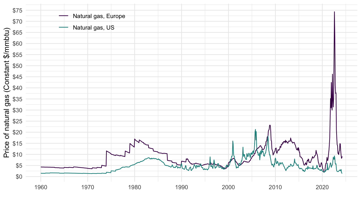

Log

All

Code

plot_log <- CMO %>%
  filter(Variable %in% c("Natural gas, US", "Natural gas, Europe")) %>%
  left_join(CPIAUCSL, by = "date") %>%
  arrange(desc(date)) %>%
  filter(!is.na(CPIAUCSL)) %>%
  mutate(value = value*CPIAUCSL[1]/CPIAUCSL) %>%
  ggplot + geom_line(aes(x = date, y = value, color = Variable)) +
  labs(x = "", y = "Price of natural gas (Constant $/mmbtu)") + theme_minimal() +
  scale_x_date(breaks = seq(1920, 2025, 10) %>% paste0("-01-01") %>% as.Date,
               labels = date_format("%Y")) +
  scale_color_manual(values = viridis(3)[1:2]) +
  theme(legend.position = c(0.2, 0.9),
        legend.title = element_blank()) +
  scale_y_log10(breaks = c(1, 2, 3, 4, 5, 8, 10, 15, 20, 30, 40, 50),
                     labels = dollar_format(a = 1))

plot_log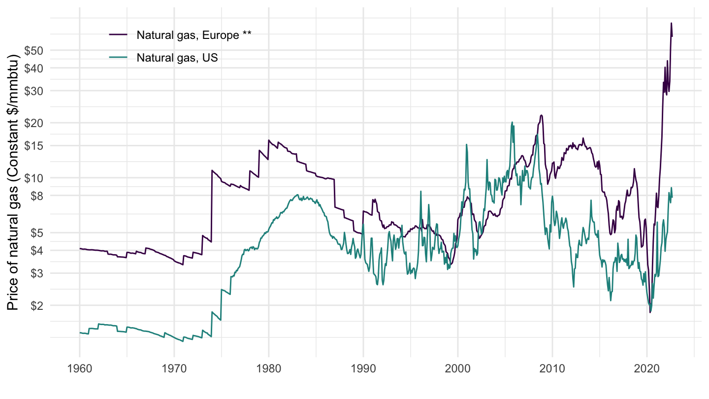

1990-

Code

CMO %>%
  filter(Variable %in% c("Natural gas, US", "Natural gas, Europe")) %>%
  left_join(CPIAUCSL, by = "date") %>%
  arrange(desc(date)) %>%
  filter(!is.na(CPIAUCSL)) %>%
  filter(date >= as.Date("1990-01-01")) %>%
  mutate(value = value*CPIAUCSL[1]/CPIAUCSL) %>%
  ggplot + geom_line(aes(x = date, y = value, color = Variable)) +
  labs(x = "", y = "Price of natural gas (Constant $/mmbtu)") + theme_minimal() +
  scale_x_date(breaks = seq(1920, 2025, 5) %>% paste0("-01-01") %>% as.Date,
               labels = date_format("%Y")) +
  scale_color_manual(values = viridis(3)[1:2]) +
  theme(legend.position = c(0.2, 0.9),
        legend.title = element_blank()) +
  scale_y_log10(breaks = c(1, 2, 3, 4, 5, 8, 10, 15, 20, 30, 40, 50),
                     labels = dollar_format(a = 1))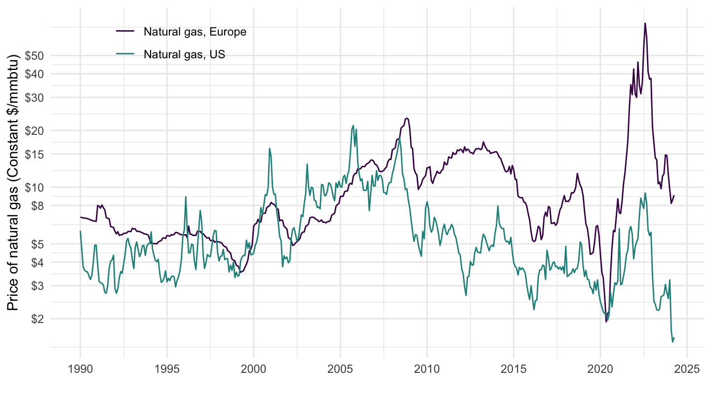

2000-

Code

CMO %>%
  filter(Variable %in% c("Natural gas, US", "Natural gas, Europe")) %>%
  left_join(CPIAUCSL, by = "date") %>%
  arrange(desc(date)) %>%
  filter(!is.na(CPIAUCSL)) %>%
  filter(date >= as.Date("2000-01-01")) %>%
  mutate(value = value*CPIAUCSL[1]/CPIAUCSL) %>%
  ggplot + geom_line(aes(x = date, y = value, color = Variable)) +
  labs(x = "", y = "Price of natural gas (Constant $/mmbtu)") + theme_minimal() +
  scale_x_date(breaks = seq(1920, 2025, 2) %>% paste0("-01-01") %>% as.Date,
               labels = date_format("%Y")) +
  scale_color_manual(values = viridis(3)[1:2]) +
  theme(legend.position = c(0.2, 0.9),
        legend.title = element_blank()) +
  scale_y_log10(breaks = c(1, 2, 3, 4, 5, 8, 10, 15, 20, 30, 40, 50, 80),
                     labels = dollar_format(a = 1))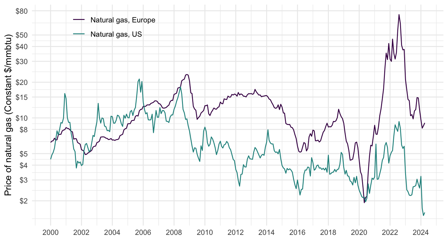

1999-

Linear

Code

plot_linear <- CMO %>%
  filter(Variable %in% c("Natural gas, US", "Natural gas, Europe")) %>%
  arrange(desc(date)) %>%
  filter(date >= as.Date("1999-01-01")) %>%
  mutate(country = case_when(Variable == "Natural gas, US" ~ "États-Unis",
                             Variable == "Natural gas, Europe" ~ "Europe",
                             T ~ NA))  %>%
  ggplot + geom_line(aes(x = date, y = value, color = country)) +
  labs(x = "", y = "") + theme_minimal() +
  scale_x_date(breaks = c(seq(1999, 2100, 2)) %>% paste0("-01-01") %>% as.Date,
               labels = date_format("%Y")) +
  scale_color_manual(values = c("#B22234", "#003399")) +
  theme(legend.position = c(0.2, 0.9),
        legend.title = element_blank(),
        axis.text.x = element_text(angle = 45, vjust = 1, hjust = 1)) +
  scale_y_continuous(breaks = seq(0, 100, 5),
                     labels = dollar_format(a = 1)) +
  labs(caption = "")
  

plot <- plot_linear
plot_linear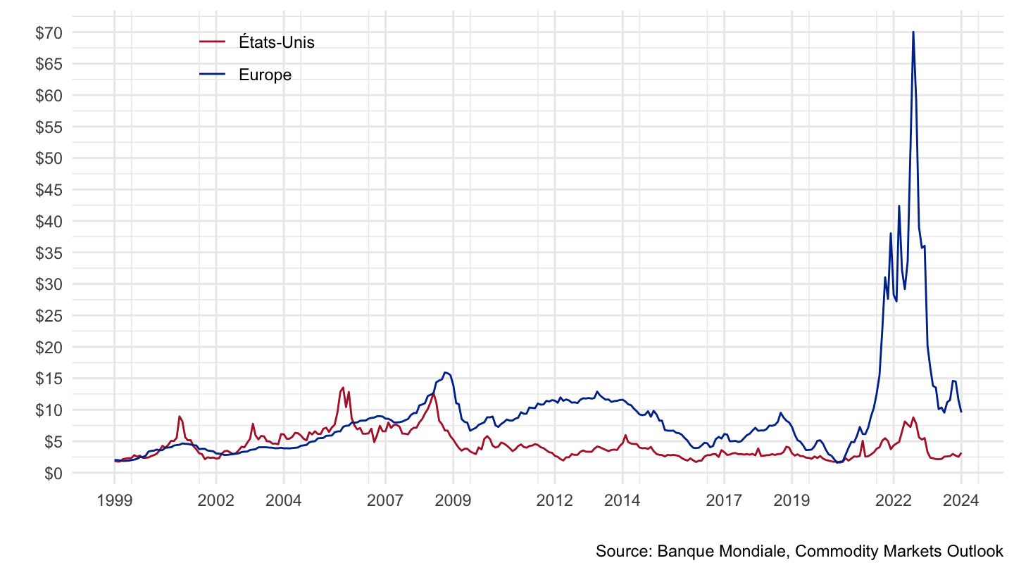

Code

save(plot, file = "CMO_files/figure-html/natural-gas-real-linear-1999-1.RData")

Log

Code

plot_log <- plot_linear +
  scale_y_log10(breaks = c(1, 2, 3, 4, 5, 8, 10, 15, 20, 30, 40, 50, 80),
                     labels = dollar_format(a = 1))

plot <- plot_log
save(plot, file = "CMO_files/figure-html/natural-gas-real-log-1999-1.RData")
plot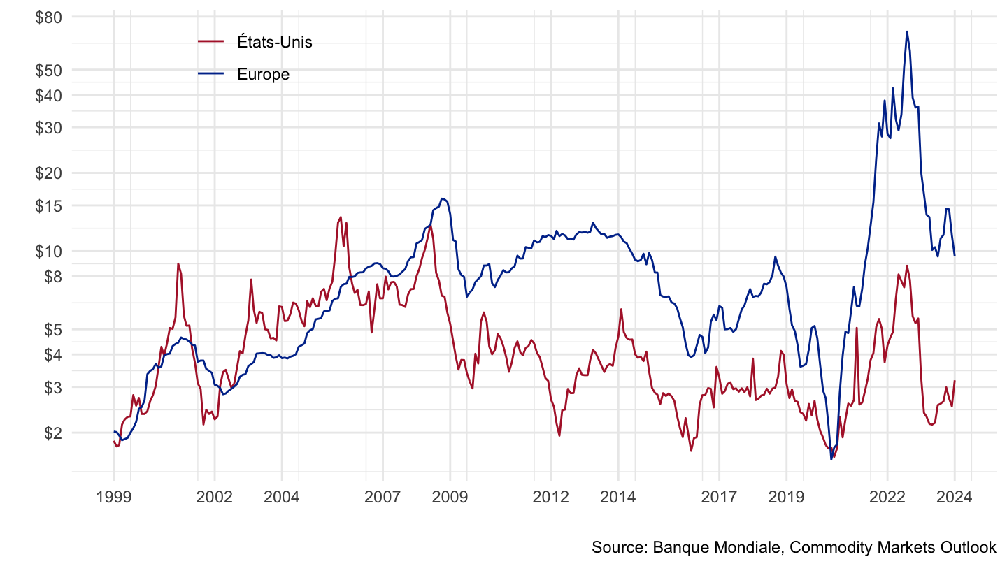

Both

Code

plot_both <- ggarrange(plot_linear + ggtitle("Linear Scale"), plot_log  + ggtitle("Log Scale"), common.legend = T)

plot <- plot_both
save(plot, file = "CMO_files/figure-html/natural-gas-real-both-1999-1.RData")
plot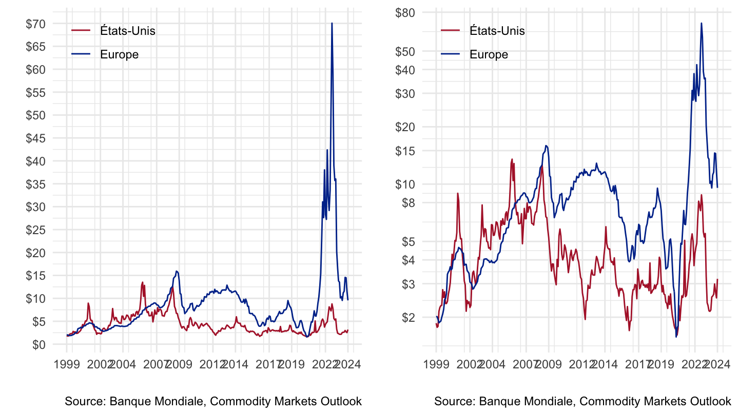

Bind

Code

ggarrange(plot_linear + ggtitle("Linear Scale"), plot_log  + ggtitle("Log Scale"), common.legend = T)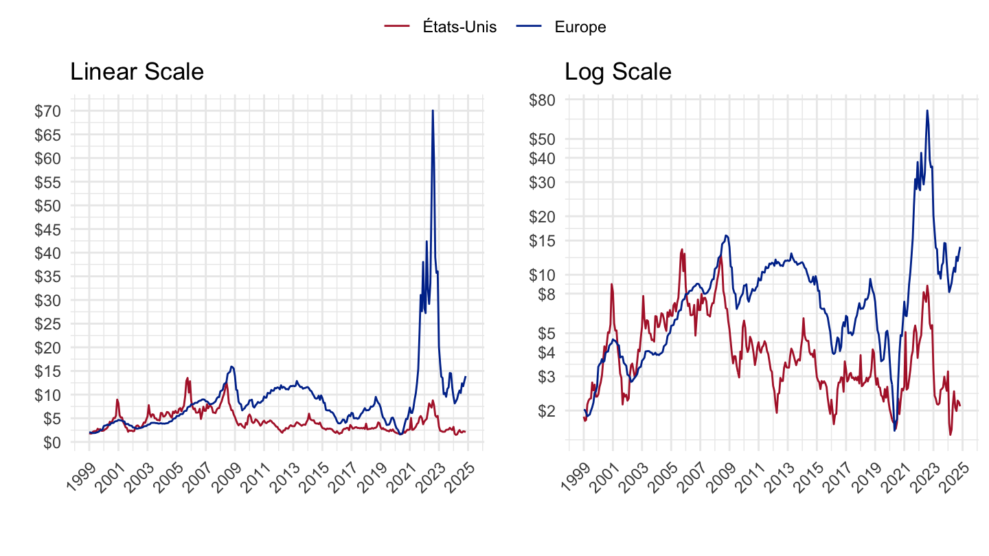

Wheat Prices

Nominal prices

Linear

Code

plot_linear <- CMO %>%
  filter(Variable %in% c("Wheat, US HRW", "Wheat, US SRW")) %>%
  ggplot + geom_line(aes(x = date, y = value, color = Variable)) +
  labs(x = "", y = "Price of wheat (Current $/mt)") + theme_minimal() +
  scale_x_date(breaks = seq(1920, 2025, 10) %>% paste0("-01-01") %>% as.Date,
               labels = date_format("%Y")) +
  scale_color_manual(values = viridis(3)[1:2]) +
  theme(legend.position = c(0.4, 0.8),
        legend.title = element_blank()) +
  scale_y_continuous(breaks = seq(0, 2000, 50),
                     labels = dollar_format(a = 1))

plot_linear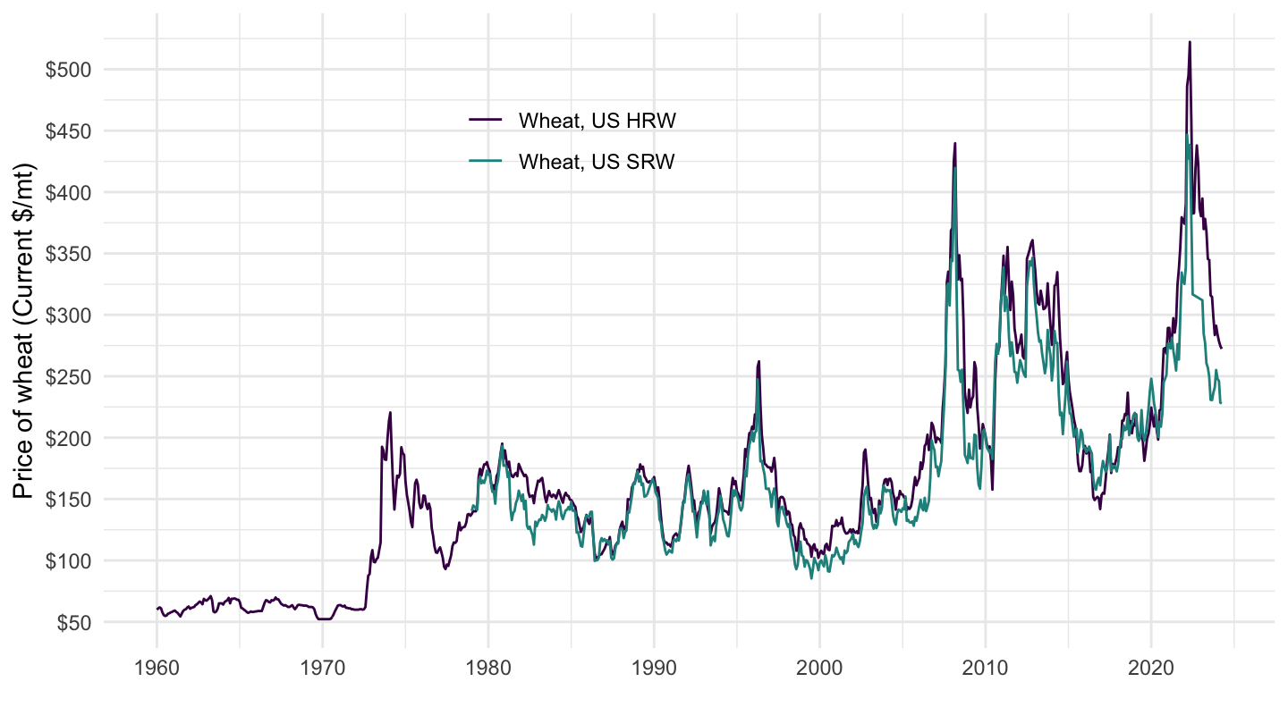

Log

Code

plot_log <- CMO %>%
  filter(Variable %in% c("Wheat, US HRW", "Wheat, US SRW")) %>%
  ggplot + geom_line(aes(x = date, y = value, color = Variable)) +
  labs(x = "", y = "Price of wheat (Current $/mt)") + theme_minimal() +
  scale_x_date(breaks = seq(1920, 2025, 10) %>% paste0("-01-01") %>% as.Date,
               labels = date_format("%Y")) +
  scale_color_manual(values = viridis(3)[1:2]) +
  theme(legend.position = c(0.4, 0.8),
        legend.title = element_blank()) +
  scale_y_log10(breaks = 100*c(0.1, 0.2, 0.3, 0.5, 0.8, 1, 1.5, 2, 3, 4, 5, 7, 8, 10, 12, 14, 20, 30, 40, 50, 80),
                     labels = dollar_format(a = 1))

plot_log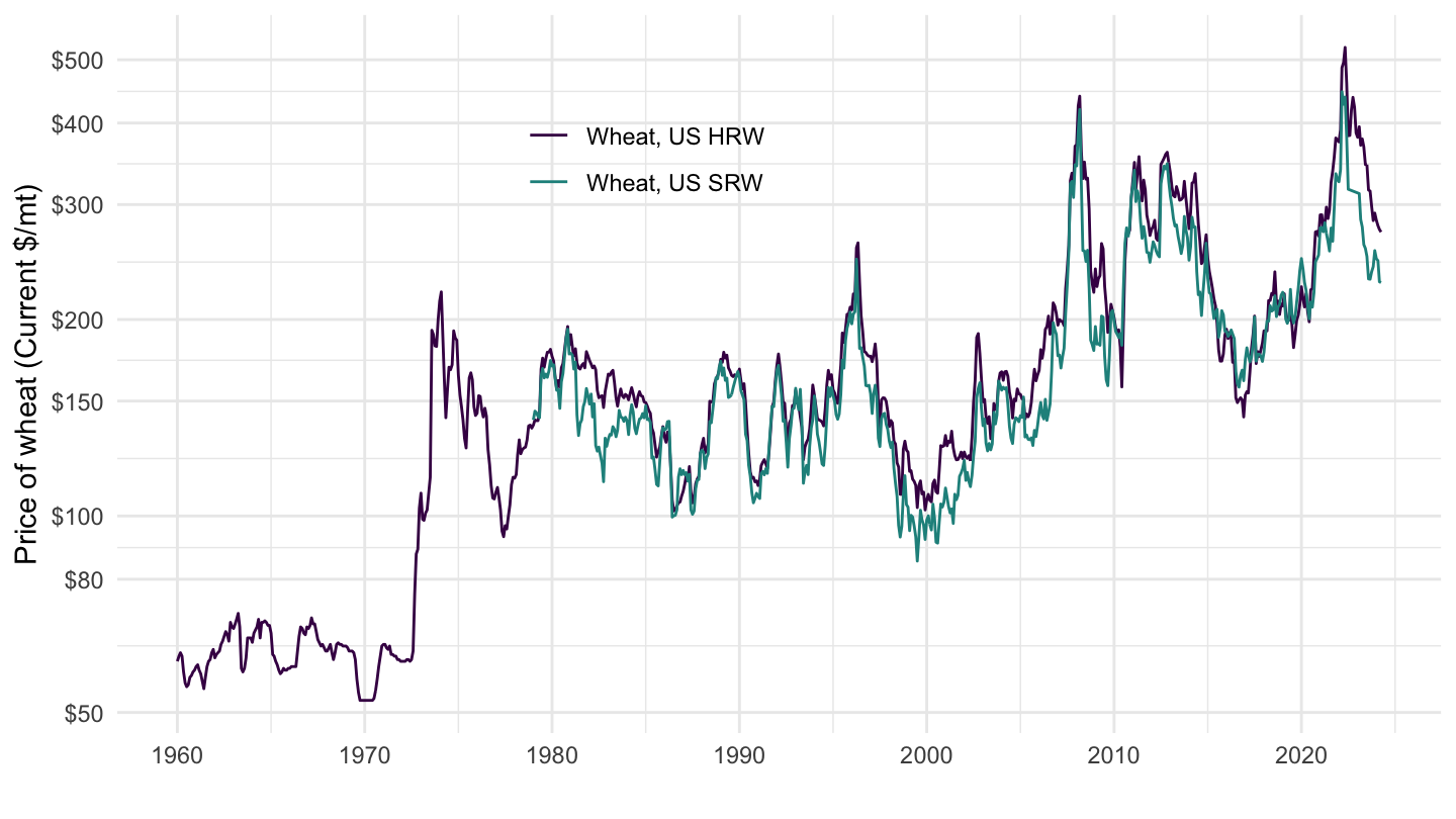

Bind

Code

ggarrange(plot_linear + ggtitle("Linear Scale"), plot_log  + ggtitle("Log Scale"), common.legend = T)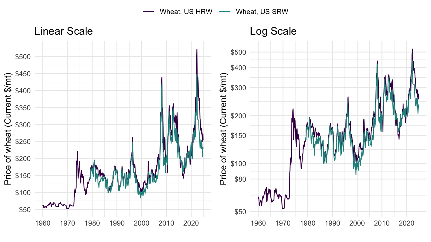

Real prices

Linear

Code

plot_linear <- CMO %>%
  filter(Variable %in% c("Wheat, US HRW", "Wheat, US SRW")) %>%
  left_join(CPIAUCSL, by = "date") %>%
  arrange(desc(date)) %>%
  filter(!is.na(CPIAUCSL)) %>%
  mutate(value = value*CPIAUCSL[1]/CPIAUCSL) %>%
  ggplot + geom_line(aes(x = date, y = value, color = Variable)) +
  labs(x = "", y = "Price of wheat (Current $/mt)") + theme_minimal() +
  scale_x_date(breaks = seq(1920, 2025, 10) %>% paste0("-01-01") %>% as.Date,
               labels = date_format("%Y")) +
  scale_color_manual(values = viridis(3)[1:2]) +
  theme(legend.position = c(0.8, 0.9),
        legend.title = element_blank()) +
  scale_y_continuous(breaks = seq(0, 2000, 50),
                     labels = dollar_format(a = 1))

plot_linear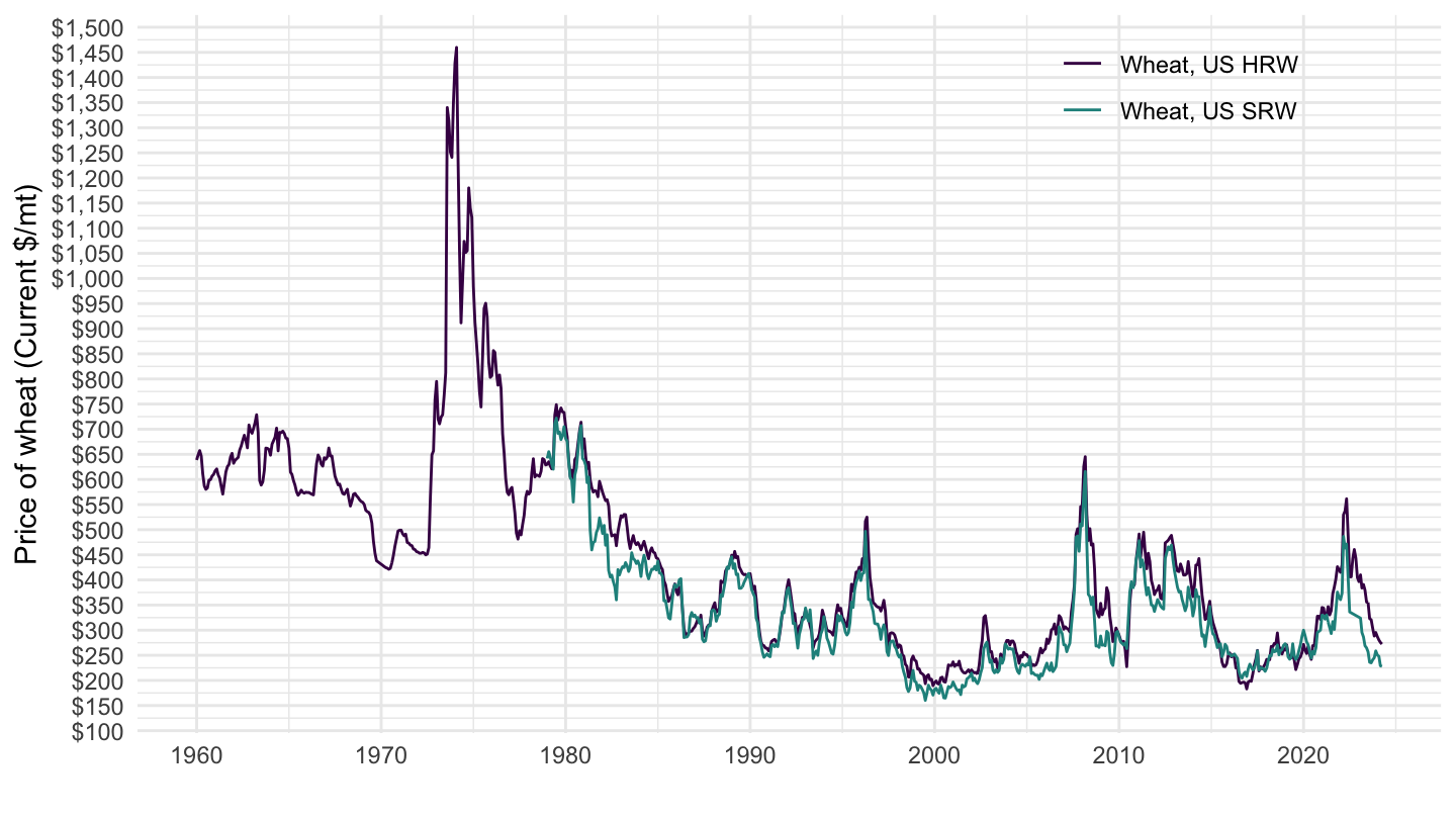

Log

Code

plot_log <- CMO %>%
  filter(Variable %in% c("Wheat, US HRW", "Wheat, US SRW")) %>%
  left_join(CPIAUCSL, by = "date") %>%
  arrange(desc(date)) %>%
  filter(!is.na(CPIAUCSL)) %>%
  mutate(value = value*CPIAUCSL[1]/CPIAUCSL) %>%
  ggplot + geom_line(aes(x = date, y = value, color = Variable)) +
  labs(x = "", y = "Price of wheat (Current $/mt)") + theme_minimal() +
  scale_x_date(breaks = seq(1920, 2025, 10) %>% paste0("-01-01") %>% as.Date,
               labels = date_format("%Y")) +
  scale_color_manual(values = viridis(3)[1:2]) +
  theme(legend.position = c(0.8, 0.9),
        legend.title = element_blank()) +
  scale_y_log10(breaks = 100*c(0.1, 0.2, 0.3, 0.5, 0.8, 1, 1.5, 2, 3, 4, 5,  8, 10, 12, 14, 20, 30, 40, 50),
                     labels = dollar_format(a = 1))

plot_log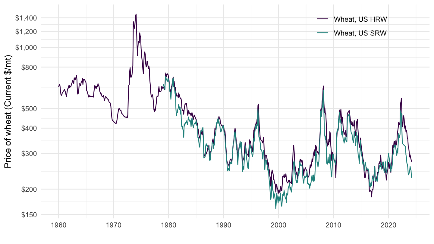

Bind

Code

ggarrange(plot_linear + ggtitle("Linear Scale"), plot_log  + ggtitle("Log Scale"), common.legend = T)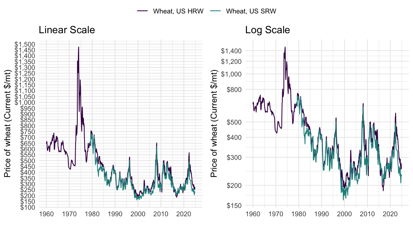

Oil

Nominal prices

Linear

Code

plot_linear <- CMO %>%
  filter(Variable %in% c("Crude oil, Dubai", "Crude oil, WTI")) %>%
  ggplot + geom_line(aes(x = date, y = value, color = Variable)) +
  labs(x = "", y = "Price of oil ($/bbl)") + theme_minimal() +
  scale_x_date(breaks = seq(1920, 2025, 10) %>% paste0("-01-01") %>% as.Date,
               labels = date_format("%Y")) +
  scale_color_manual(values = viridis(3)[1:2]) +
  theme(legend.position = c(0.4, 0.8),
        legend.title = element_blank()) +
  scale_y_continuous(breaks = seq(-20, 400, 10),
                     labels = dollar_format(a = 1))

plot_linear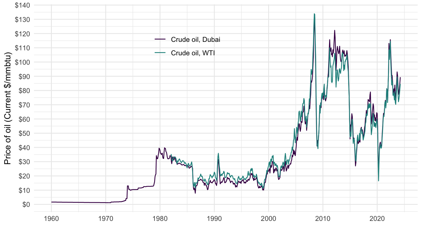

Log

Code

plot_log <- CMO %>%
  filter(Variable %in% c("Crude oil, Dubai", "Crude oil, WTI")) %>%
  ggplot + geom_line(aes(x = date, y = value, color = Variable)) +
  labs(x = "", y = "Price of oil ($/bbl)") + theme_minimal() +
  scale_x_date(breaks = seq(1920, 2025, 10) %>% paste0("-01-01") %>% as.Date,
               labels = date_format("%Y")) +
  scale_color_manual(values = viridis(3)[1:2]) +
  theme(legend.position = c(0.4, 0.8),
        legend.title = element_blank()) +
  scale_y_log10(breaks = c(1, 2, 3, 4, 5, 8, 10, 15, 20, 30, 40, 50, 80, 100, 200, 300, 500),
                     labels = dollar_format(a = 1))

plot_log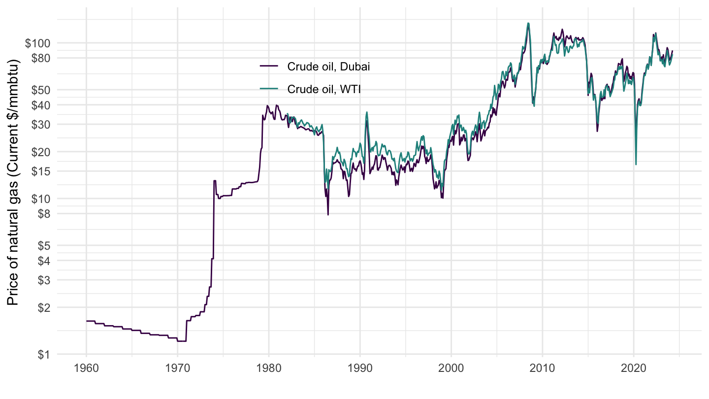

Bind

Code

ggarrange(plot_linear + ggtitle("Linear Scale"), plot_log  + ggtitle("Log Scale"), common.legend = T)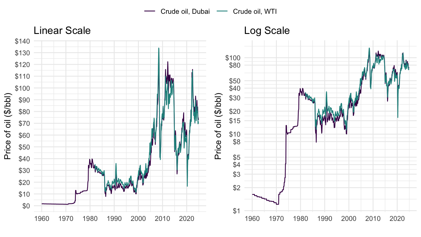

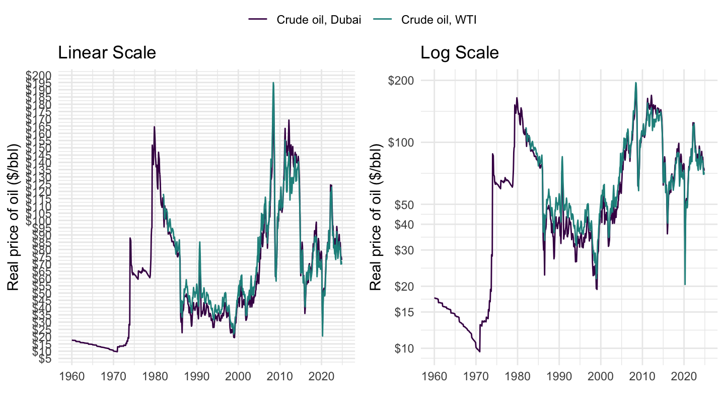
Real prices

Linear

Code

plot_linear <- CMO %>%
  filter(Variable %in% c("Crude oil, Dubai", "Crude oil, WTI")) %>%
  left_join(CPIAUCSL, by = "date") %>%
  arrange(desc(date)) %>%
  filter(!is.na(CPIAUCSL)) %>%
  mutate(value = value*CPIAUCSL[1]/CPIAUCSL) %>%
  ggplot + geom_line(aes(x = date, y = value, color = Variable)) +
  labs(x = "", y = "Real price of oil ($/bbl)") + theme_minimal() +
  scale_x_date(breaks = seq(1920, 2025, 10) %>% paste0("-01-01") %>% as.Date,
               labels = date_format("%Y")) +
  scale_color_manual(values = viridis(3)[1:2]) +
  theme(legend.position = c(0.2, 0.9),
        legend.title = element_blank()) +
  scale_y_continuous(breaks = seq(-20, 400, 5),
                     labels = dollar_format(a = 1))

plot_linear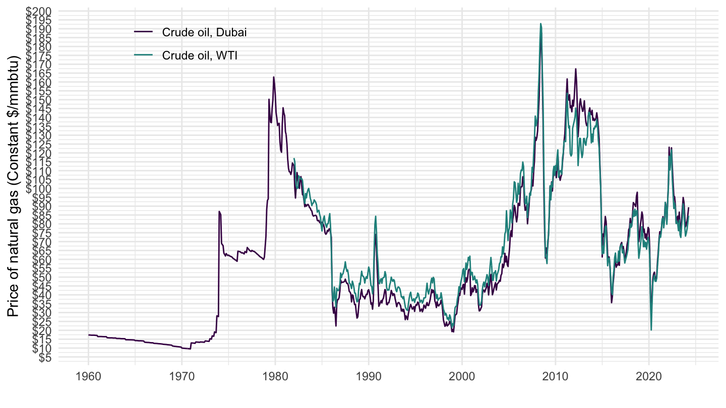

Log

Code

plot_log <- CMO %>%
  filter(Variable %in% c("Crude oil, Dubai", "Crude oil, WTI")) %>%
  left_join(CPIAUCSL, by = "date") %>%
  arrange(desc(date)) %>%
  filter(!is.na(CPIAUCSL)) %>%
  mutate(value = value*CPIAUCSL[1]/CPIAUCSL) %>%
  ggplot + geom_line(aes(x = date, y = value, color = Variable)) +
  labs(x = "", y = "Real price of oil ($/bbl)") + theme_minimal() +
  scale_x_date(breaks = seq(1920, 2025, 10) %>% paste0("-01-01") %>% as.Date,
               labels = date_format("%Y")) +
  scale_color_manual(values = viridis(3)[1:2]) +
  theme(legend.position = c(0.2, 0.9),
        legend.title = element_blank()) +
  scale_y_log10(breaks = c(1, 2, 3, 4, 5, 8, 10, 15, 20, 30, 40, 50, 100, 200, 300, 500),
                     labels = dollar_format(a = 1))

plot_log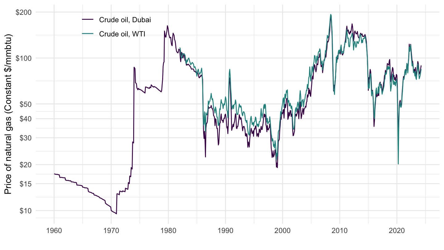

Bind

Code

ggarrange(plot_linear + ggtitle("Linear Scale"), plot_log  + ggtitle("Log Scale"), common.legend = T)

Info

Links

Data on energy

Data on industry

LAST_COMPILE

Last

variable

Natural Gas: Europe and US

Nominal prices

Linear

Log

All

1990-

2000-

Bind

Real prices

Linear

Log

All

1990-

2000-

1999-

Linear

Log

Both

Bind

Wheat Prices

Nominal prices

Linear

Log

Bind

Real prices

Linear

Log

Bind

Oil

Nominal prices

Linear

Log

Bind

Real prices

Linear

Log

Bind