Non-household consumption volumes of gas by consumption bands

Data - Eurostat

Author

Info

Related energy datasets

source	dataset	Title	Download	Compile
eurostat	nrg_pc_203_v	Non-household consumption volumes of gas by consumption bands	2024-09-18	[2024-09-15]
ec	WOB	Weekly Oil Bulletin	2024-08-25	[2024-09-15]
eurostat	ei_isen_m	Energy - monthly data	2024-09-14	[2024-09-18]
eurostat	nrg_bal_c	Complete energy balances	2024-09-15	[2023-12-31]
eurostat	nrg_pc_202	Gas prices for household consumers - bi-annual data (from 2007 onwards)	2024-09-18	[2024-09-19]
eurostat	nrg_pc_203	Gas prices for non-household consumers - bi-annual data (from 2007 onwards)	2024-09-18	[2023-06-11]
eurostat	nrg_pc_203_c	Gas prices components for non-household consumers - annual data	2024-09-15	[2024-09-19]
eurostat	nrg_pc_203_h	Gas prices for industrial consumers - bi-annual data (until 2007)	2024-09-15	[2024-09-19]
eurostat	nrg_pc_204	Electricity prices for household consumers - bi-annual data (from 2007 onwards)	2024-09-15	[2024-09-15]
eurostat	nrg_pc_205	Electricity prices for non-household consumers - bi-annual data (from 2007 onwards)	2024-09-18	[2023-06-11]
fred	energy	Energy	2024-09-18	[2024-09-18]
iea	world_energy_balances_highlights_2022	World Energy Balances Highlights (2022 edition)	2023-04-24	[2024-06-20]
wb	CMO	World Bank Commodity Price Data (The Pink Sheet)	2024-05-23	[2024-06-20]
wdi	EG.GDP.PUSE.KO.PP.KD	GDP per unit of energy use (constant 2017 PPP $ per kg of oil equivalent)	2024-09-18	[2024-09-18]
wdi	EG.USE.PCAP.KG.OE	Energy use (kg of oil equivalent per capita)	2024-09-18	[2024-09-18]
yahoo	energy	Energy	2024-09-18	[2024-09-18]

LAST_COMPILE

LAST_COMPILE
2024-09-19

Last

Code

nrg_pc_203_v %>%
  group_by(time) %>%
  summarise(Nobs = n()) %>%
  arrange(desc(time)) %>%
  head(1) %>%
  print_table_conditional()

time	Nobs
2023	180

Info

Electricity and gas prices in the first half of 2022. html / png

Code

include_graphics("https://ec.europa.eu/eurostat/documents/4187653/14185664/Gas+and+Electricity+Prices+S1_2022.png")

nrg_cons

Code

nrg_pc_203_v %>%
  left_join(nrg_cons, by = "nrg_cons") %>%
  group_by(nrg_cons, Nrg_cons) %>%
  summarise(Nobs = n()) %>%
  arrange(-Nobs) %>%
  print_table_conditional()

nrg_cons	Nrg_cons	Nobs
GJ100000-999999	Consumption from 100 000 GJ to 999 999 GJ - band I4	227
GJ_LT1000	Consumption less than 1 000 GJ - band I1	227
GJ1000-9999	Consumption from 1 000 GJ to 9 999 GJ -band I2	221
GJ10000-99999	Consumption from 10 000 GJ to 99 999 GJ - band I3	221
GJ1000000-3999999	Consumption from 1 000 000 GJ to 3 999 999 GJ - band I5	204
GJ_GE4000000	Consumption 4 000 000 GJ or over - band I6	155

geo

Code

nrg_pc_203_v %>%
  left_join(geo, by = "geo") %>%
  group_by(geo, Geo) %>%
  summarise(Nobs = n()) %>%
  arrange(-Nobs) %>%
  mutate(Geo = ifelse(geo == "DE", "Germany", Geo)) %>%
  mutate(Flag = gsub(" ", "-", str_to_lower(Geo)),
         Flag = paste0('<img src="../../bib/flags/vsmall/', Flag, '.png" alt="Flag">')) %>%
  select(Flag, everything()) %>%
  {if (is_html_output()) datatable(., filter = 'top', rownames = F, escape = F) else .}

time

Code

nrg_pc_203_v %>%
  group_by(time) %>%
  summarise(Nobs = n()) %>%
  arrange(desc(time)) %>%
  print_table_conditional()

time	Nobs
2023	180
2022	188
2021	182
2020	187
2019	187
2018	175
2017	156

Example

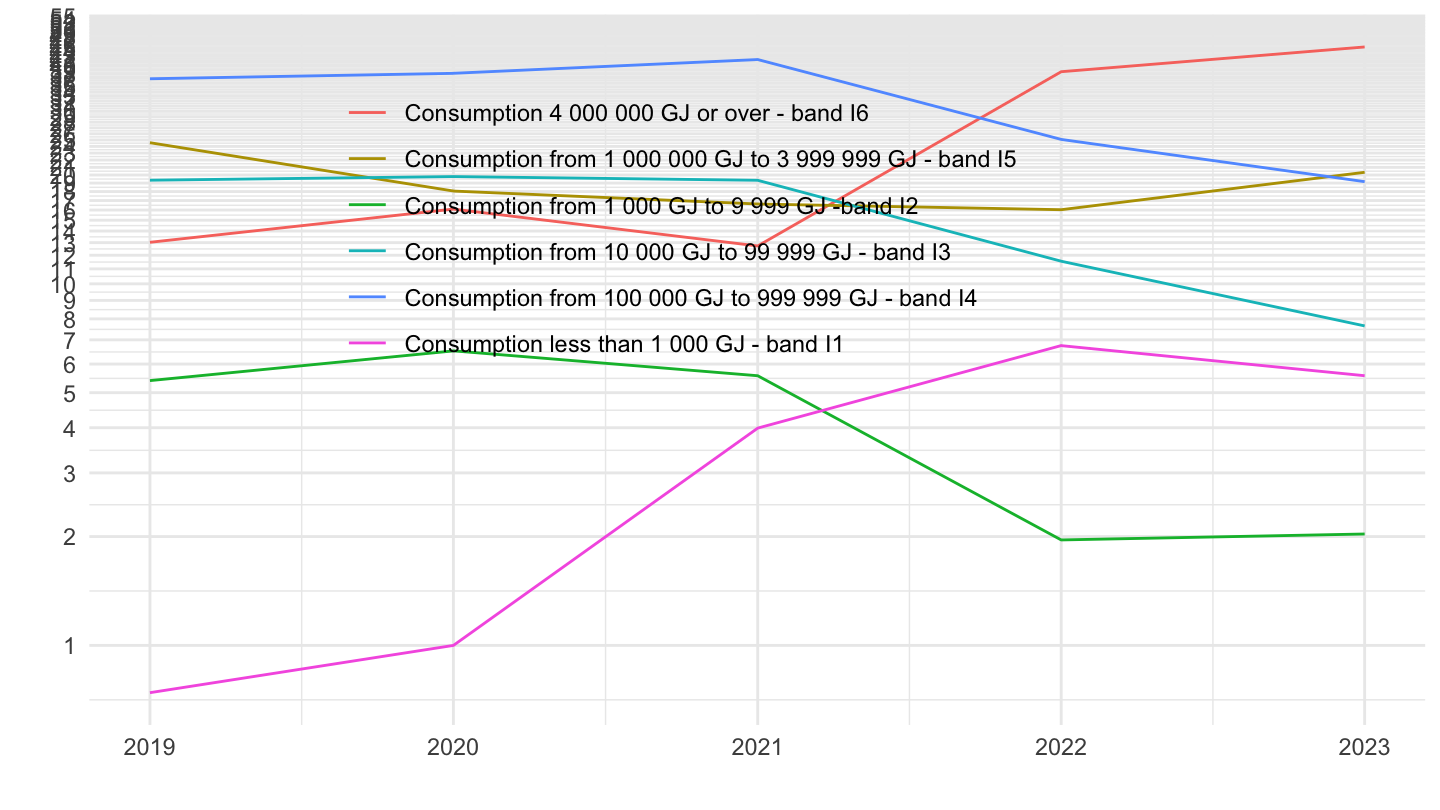
France

Code

nrg_pc_203_v %>%
  filter(geo == "FR") %>%
  left_join(nrg_cons, by = "nrg_cons") %>%
  select_if(~ n_distinct(.) > 1) %>%
  year_to_date %>%
  ggplot + geom_line(aes(x = date, y = values, color = Nrg_cons)) +
  theme_minimal() + xlab("") + ylab("") +
  scale_x_date(breaks = seq(1920, 2025, 1) %>% paste0("-01-01") %>% as.Date,
               labels = date_format("%Y")) +
  scale_y_log10(breaks = seq(1, 100, 1)) +
  theme(legend.position = c(0.45, 0.7),
        legend.title = element_blank())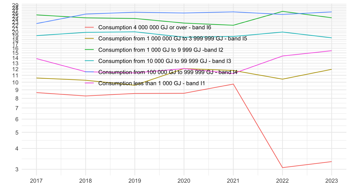

Germany

Code

nrg_pc_203_v %>%
  filter(geo == "DE") %>%
  left_join(nrg_cons, by = "nrg_cons") %>%
  select_if(~ n_distinct(.) > 1) %>%
  year_to_date %>%
  ggplot + geom_line(aes(x = date, y = values, color = Nrg_cons)) +
  theme_minimal() + xlab("") + ylab("") +
  scale_x_date(breaks = seq(1920, 2025, 1) %>% paste0("-01-01") %>% as.Date,
               labels = date_format("%Y")) +
  scale_y_log10(breaks = seq(1, 100, 1)) +
  theme(legend.position = c(0.45, 0.7),
        legend.title = element_blank())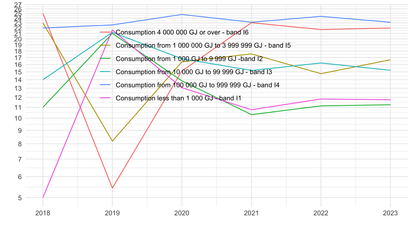

Italy

Code

nrg_pc_203_v %>%
  filter(geo == "IT") %>%
  left_join(nrg_cons, by = "nrg_cons") %>%
  select_if(~ n_distinct(.) > 1) %>%
  year_to_date %>%
  ggplot + geom_line(aes(x = date, y = values, color = Nrg_cons)) +
  theme_minimal() + xlab("") + ylab("") +
  scale_x_date(breaks = seq(1920, 2025, 1) %>% paste0("-01-01") %>% as.Date,
               labels = date_format("%Y")) +
  scale_y_log10(breaks = seq(1, 100, 1)) +
  theme(legend.position = c(0.45, 0.7),
        legend.title = element_blank())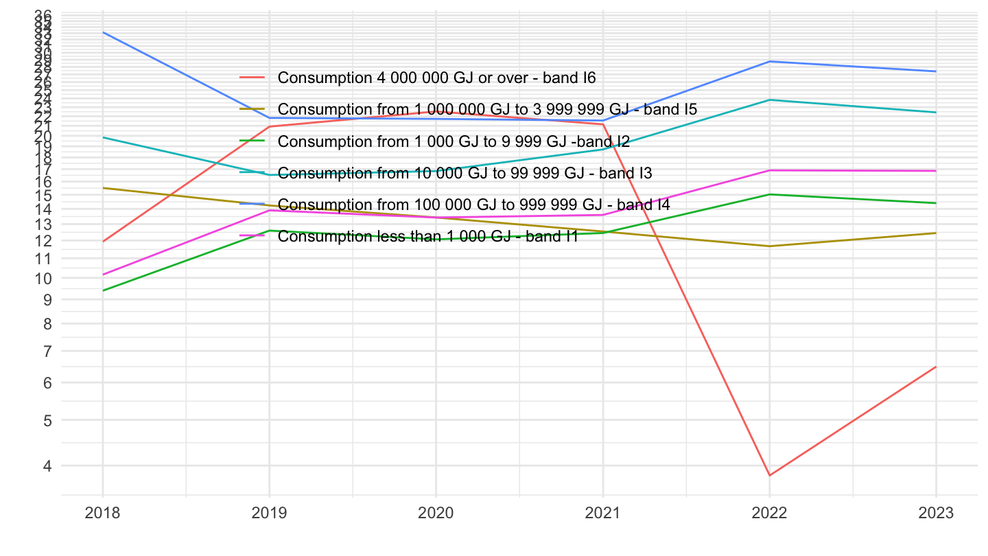

Spain

Code

nrg_pc_203_v %>%
  filter(geo == "ES") %>%
  left_join(nrg_cons, by = "nrg_cons") %>%
  select_if(~ n_distinct(.) > 1) %>%
  year_to_date %>%
  ggplot + geom_line(aes(x = date, y = values, color = Nrg_cons)) +
  theme_minimal() + xlab("") + ylab("") +
  scale_x_date(breaks = seq(1920, 2025, 1) %>% paste0("-01-01") %>% as.Date,
               labels = date_format("%Y")) +
  scale_y_log10(breaks = seq(1, 100, 1)) +
  theme(legend.position = c(0.45, 0.7),
        legend.title = element_blank())