Electricity prices for household consumers - bi-annual data (from 2007 onwards) - nrg_pc_204

Name: Electricity prices for household consumers - bi-annual data (from 2007 onwards)
Creator: François Geerolf
License: https://creativecommons.org/licenses/by/4.0/

Data - Eurostat

Author

François Geerolf

Last observation: H2 2025 (N = 2052)

First observation: H1 2007 (N = 294)

Last data update: 13 août 2026, 02:18

Last compile: 05 sept. 2026, 00:40

Structure

Info

Electricity and gas prices in the first half of 2022. html / png

Code

include_graphics("https://ec.europa.eu/eurostat/documents/4187653/14185664/Gas+and+Electricity+Prices+S1_2022.png")

html
Electricity prices for household consumers, second half 2022. html

Code

include_graphics("https://ec.europa.eu/eurostat/statistics-explained/images/7/7a/Electricity_prices_for_household_consumers%2C_second_half_2022_v5.png")

geo

Code

nrg_pc_204 |>
  group_by(geo, Geo) |>
  summarise(Nobs = n()) |>
  arrange(-Nobs) |>
  mutate(Geo = ifelse(geo == "DE", "Germany", Geo)) |>
  mutate(Flag = gsub(" ", "-", str_to_lower(Geo)),
         Flag = paste0('<img src="../../bib/flags/vsmall/', Flag, '.png" alt="Flag">')) |>
  select(Flag, everything()) %>%
  {if (is_html_output()) datatable(., filter = 'top', rownames = F, escape = F) else .}

What do I_TAX, X_VAT, X_TAX mean ?

Netherlands

Code

nrg_pc_204 |>
  filter(geo %in% c("FR"),
         currency == "EUR",
         time %in% c("2021S2", "2022S1", "2022S2", "2023S1")) %>%
  select_if(~n_distinct(.) > 1) |>
  #mutate(values = 1000* values) %>%
  spread(tax, values) |>
  mutate(` Taxes except VAT` = X_VAT-X_TAX,
            `  VAT` = I_TAX-X_VAT,
            `Excluding taxes` = X_TAX) |>
  print_table_conditional()

Consumption < 1 000 kWh

bars

Code

nrg_pc_204 |>
  filter(geo %in% c("FR", "DE", "EA", "ES"),
         nrg_cons == "KWH_LT1000",
         currency == "EUR",
         time %in% c("2021S2", "2022S1", "2022S2", "2023S1")) %>%
  select_if(~n_distinct(.) > 1) |>
  mutate(Geo = ifelse(geo == "EA", "Europe", Geo)) |>
  spread(tax, values) |>
  transmute(time, Geo,
            ` Taxes except VAT` = X_VAT-X_TAX,
            `  VAT` = I_TAX-X_VAT,
            `Excluding taxes` = X_TAX) |>
  gather(Tax, values, - time, -Geo) |>
  ggplot(aes(x = time, y = values, fill = Tax)) + 
  geom_bar(stat = "identity",
           position = "stack") +
  facet_grid(~ Geo) + theme_minimal() +
theme(legend.position = c(0.2, 0.9),
      legend.title = element_blank()) +
  scale_fill_manual(values = viridis(3)[1:3]) +
  scale_y_continuous(breaks = seq(-30, 30, .1),
                labels = dollar_format(a = .1, pre = "", su = "€/kWh"),
                limits = c(0, 0.6))  +
  xlab("Semester") + ylab("") +
  ggtitle("Electricity price, LOW Consumption")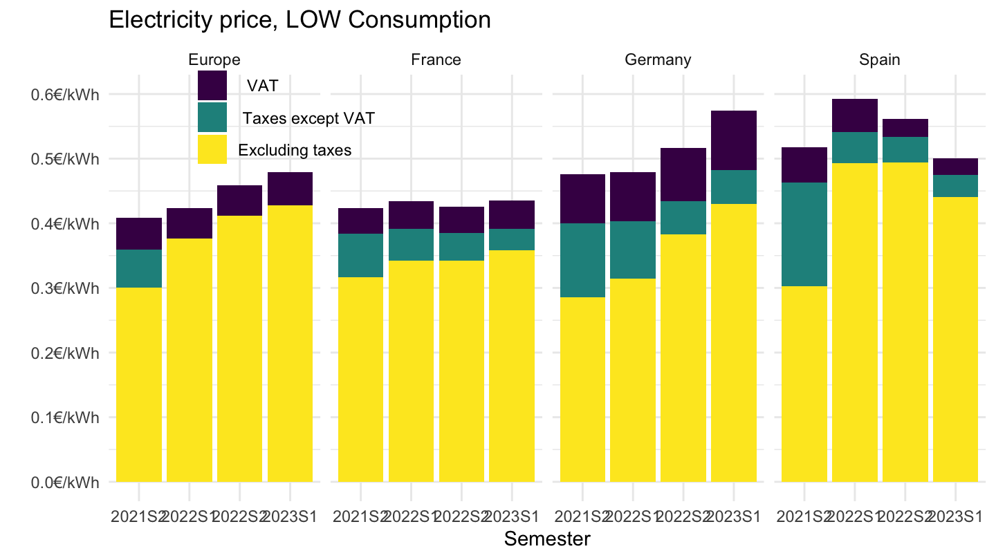

France, Germany, EA19, Spain

All

Code

nrg_pc_204 |>
  filter(geo %in% c("FR", "DE", "EA", "ES"),
         tax %in% c("I_TAX", "X_TAX"),
         nrg_cons == "KWH_LT1000",
         currency == "EUR") |>
  semester_to_date() |>
  mutate(Geo = ifelse(geo == "EA", "Europe", Geo)) |>
  add_flag_color("Geo") |>
  ggplot() + geom_line(aes(x = date, y = values, color = color, linetype = Tax)) +
  scale_color_identity() + theme_minimal()  + add_flags +
  scale_x_date(breaks = as.Date(paste0(seq(1960, 2100, 2), "-01-01")),
               labels = date_format("%Y")) +
  theme(legend.position = c(0.2, 0.8),
        legend.title = element_blank()) +
  xlab("") + ylab("Electricity Prices - C < 1 000 kWh") +
  scale_y_log10(breaks = seq(-30, 30, .1),
                labels = dollar_format(a = .1, pre = "", su = "€"))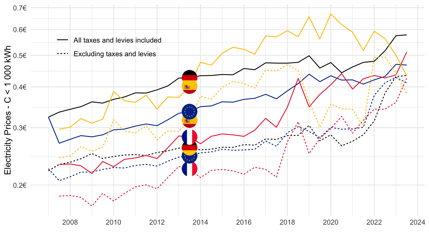

2020-

Code

nrg_pc_204 |>
  filter(geo %in% c("FR", "DE", "EA", "ES"),
         tax %in% c("I_TAX", "X_TAX"),
         nrg_cons == "KWH_LT1000",
         currency == "EUR") |>
  semester_to_date() |>
  filter(date >= as.Date("2020-01-01")) |>
  mutate(Geo = ifelse(geo == "EA", "Europe", Geo)) |>
  add_flag_color("Geo") |>
  ggplot() + geom_line(aes(x = date, y = values, color = color, linetype = Tax)) +
  scale_color_identity() + theme_minimal()  + add_flags +
  scale_x_date(breaks = as.Date(paste0(seq(1960, 2100, 1), "-01-01")),
               labels = date_format("%Y")) +
  theme(legend.position = c(0.2, 0.8),
        legend.title = element_blank()) +
  xlab("") + ylab("Band DA : Consumption < 1 000 kWh") +
  scale_y_log10(breaks = seq(-30, 30, .1),
                labels = dollar_format(a = .1, pre = "", su = "€"))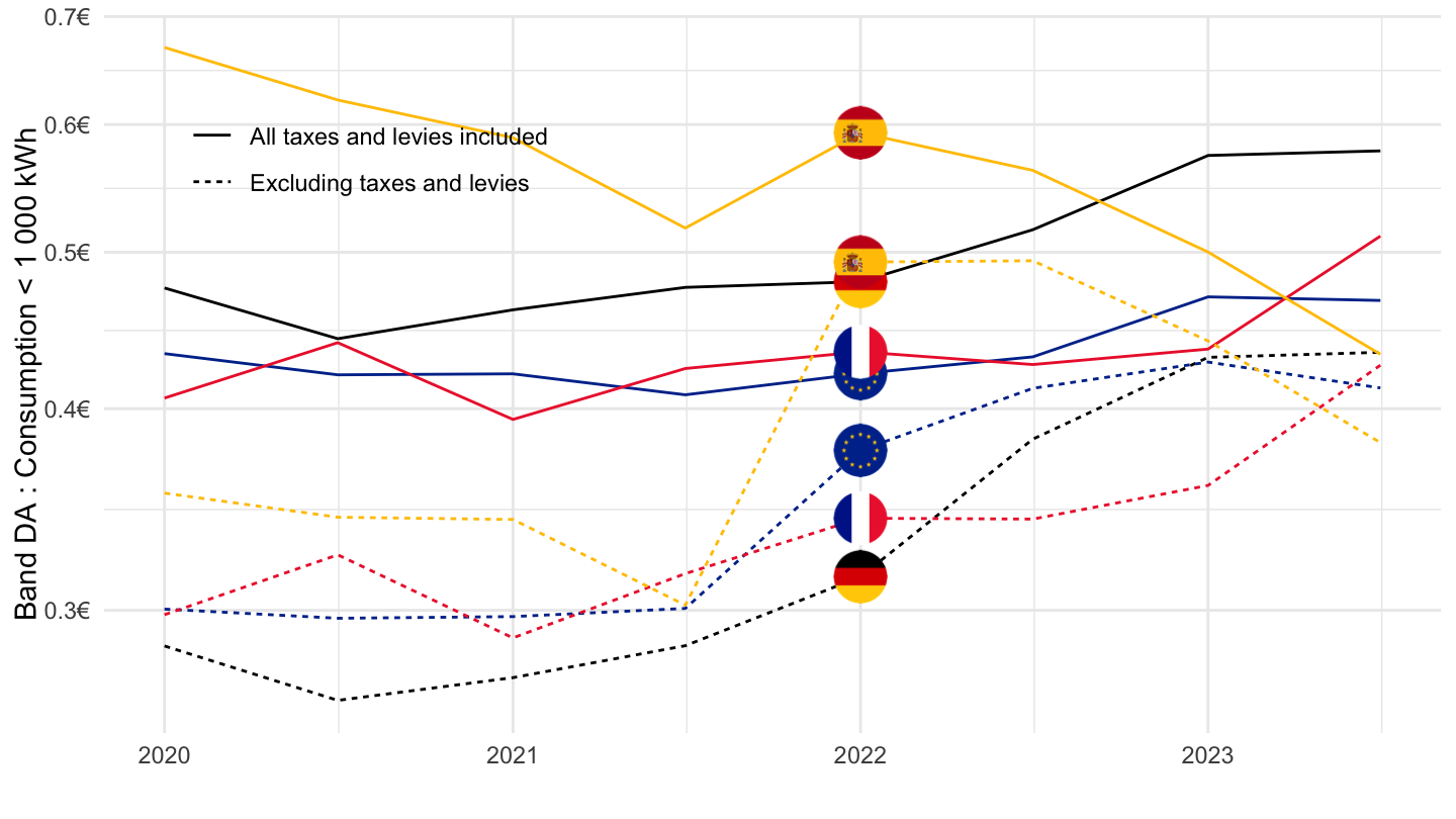

France, Germany, Italy, Spain

Code

nrg_pc_204 |>
  filter(geo %in% c("FR", "DE", "IT", "ES"),
         tax %in% c("I_TAX", "X_TAX"),
         nrg_cons == "KWH_LT1000",
         currency == "EUR") |>
  semester_to_date() |>
  filter(date >= as.Date("2020-01-01")) |>
  add_flag_color("Geo") |>
  ggplot() + geom_line(aes(x = date, y = values, color = color, linetype = Tax)) +
  scale_color_identity() + theme_minimal()  + add_flags +
  scale_x_date(breaks = as.Date(paste0(seq(1960, 2100, 1), "-01-01")),
               labels = date_format("%Y")) +
  theme(legend.position = c(0.2, 0.8),
        legend.title = element_blank()) +
  xlab("") + ylab("Electricity Prices - C < 1 000 kWh") +
  scale_y_log10(breaks = seq(-30, 30, .1),
                labels = dollar_format(a = .1, pre = "", su = "€"))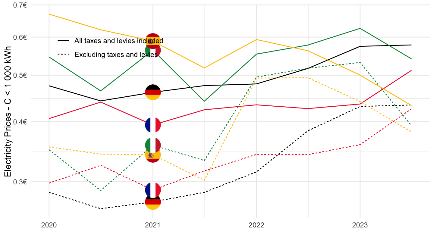

Netherlands

Code

nrg_pc_204 |>
  filter(geo %in% c("NL"),
         tax %in% c("I_TAX", "X_TAX"),
         nrg_cons == "KWH_LT1000",
         currency == "EUR") |>
  semester_to_date() |>
  add_flag_color("Geo") |>
  ggplot() + geom_line(aes(x = date, y = values, color = color, linetype = Tax)) +
  scale_color_identity() + theme_minimal()  + add_flags +
  scale_x_date(breaks = as.Date(paste0(seq(1960, 2100, 2), "-01-01")),
               labels = date_format("%Y")) +
  theme(legend.position = c(0.2, 0.3),
        legend.title = element_blank()) +
  xlab("") + ylab("Electricity Prices - C < 1 000 kWh") +
  scale_y_continuous(breaks = seq(-30, 30, .1),
                labels = dollar_format(a = .1, pre = "", su = "€"))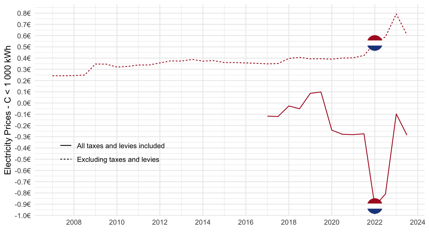

Greece, Belgium, Austria, Portugal

Code

nrg_pc_204 |>
  filter(geo %in% c("EL", "BE", "AT", "PT"),
         tax %in% c("I_TAX", "X_TAX"),
         nrg_cons == "KWH_LT1000",
         currency == "EUR") |>
  semester_to_date() |>
  add_flag_color("Geo") |>
  ggplot() + geom_line(aes(x = date, y = values, color = color, linetype = Tax)) +
  scale_color_identity() + theme_minimal()  + add_flags +
  scale_x_date(breaks = as.Date(paste0(seq(1960, 2100, 2), "-01-01")),
               labels = date_format("%Y")) +
  theme(legend.position = c(0.2, 0.9),
        legend.title = element_blank()) +
  xlab("") + ylab("Electricity Prices - C < 1 000 kWh") +
  scale_y_log10(breaks = seq(-30, 30, .1),
                labels = dollar_format(a = .1, pre = "", su = "€"))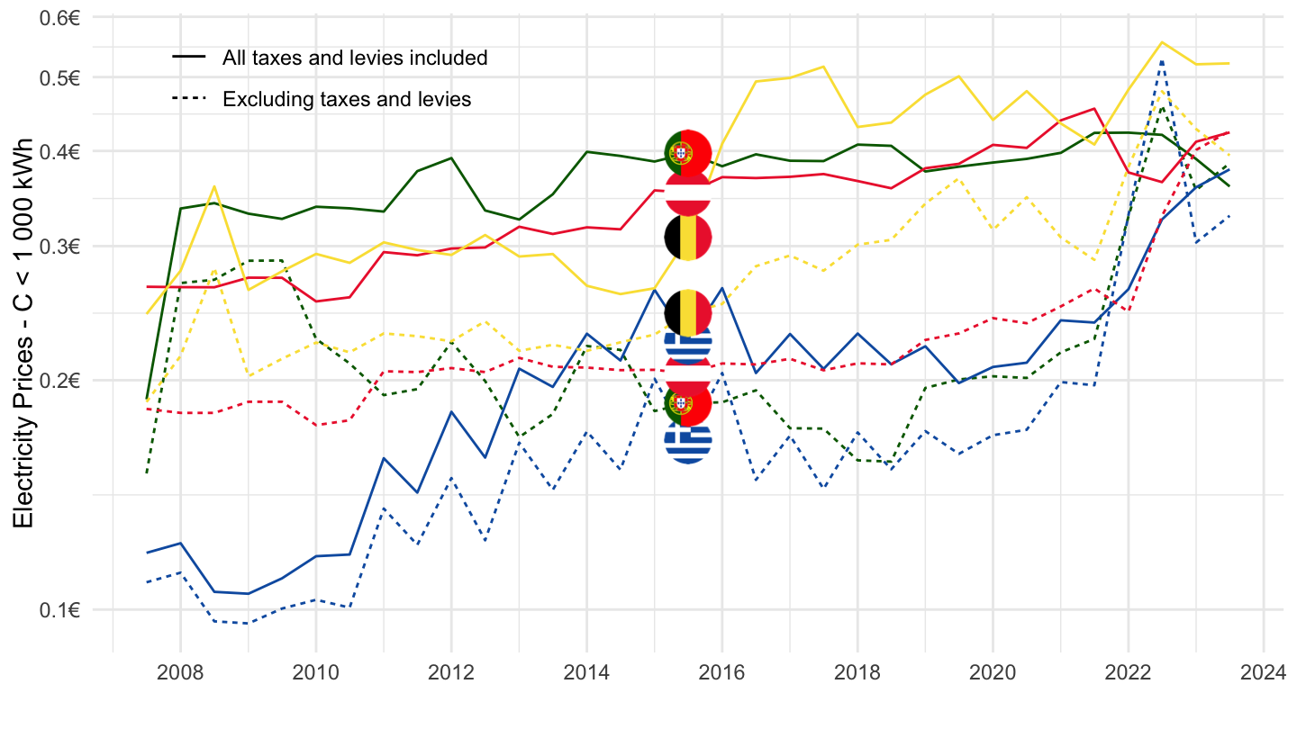

1 000 kWh < Consumption < 2 500 kWh

France, Germany, Italy, Spain

Code

nrg_pc_204 |>
  filter(geo %in% c("FR", "DE", "IT", "ES"),
         tax %in% c("I_TAX", "X_TAX"),
         nrg_cons == "KWH1000-2499",
         currency == "EUR") |>
  semester_to_date() |>
  add_flag_color("Geo") |>
  ggplot() + geom_line(aes(x = date, y = values, color = color, linetype = Tax)) +
  scale_color_identity() + theme_minimal()  + add_flags +
  scale_x_date(breaks = as.Date(paste0(seq(1960, 2100, 2), "-01-01")),
               labels = date_format("%Y")) +
  theme(legend.position = c(0.2, 0.9),
        legend.title = element_blank()) +
  xlab("") + ylab("Electricity Prices - 1 000 kWh < C < 2 500 kWh") +
  scale_y_log10(breaks = c(0.12, 0.15, 0.18, 0.2, 0.25, 0.3, 0.35),
                labels = dollar_format(a = .01, pre = "", su = "€"))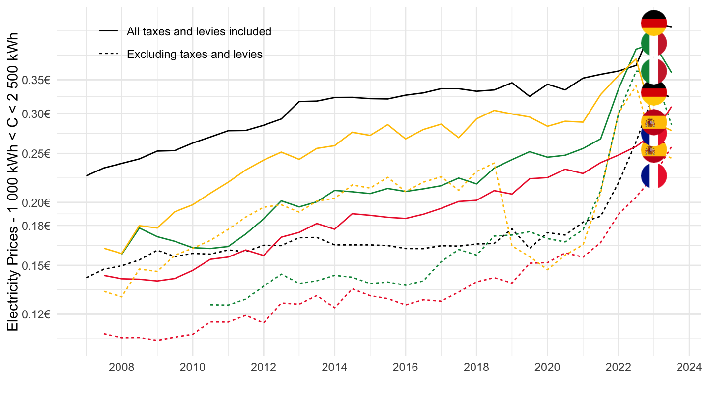

Band DE : Consumption > 15 000 kWh

France, Germany, EA19, Spain

bars

Code

nrg_pc_204 |>
  filter(geo %in% c("FR", "DE", "EA", "ES"),
         nrg_cons == "KWH_GE15000",
         currency == "EUR",
         time %in% c("2021S2", "2022S1", "2022S2")) %>%
  select_if(~n_distinct(.) > 1) |>
  mutate(Geo = ifelse(geo == "EA", "Europe", Geo)) |>
  spread(tax, values) |>
  transmute(time, Geo,
            ` Taxes except VAT` = X_VAT-X_TAX,
            `  VAT` = I_TAX-X_VAT,
            `Excluding taxes` = X_TAX) |>
  gather(Tax, values, - time, -Geo) |>
  ggplot(aes(x = time, y = values, fill = Tax)) + 
  geom_bar(stat = "identity",
           position = "stack") +
  facet_grid(~ Geo) + theme_minimal() +
theme(legend.position = "none",
      legend.title = element_blank()) +
  scale_fill_manual(values = viridis(3)[1:3]) +
  scale_y_continuous(breaks = seq(-30, 30, .1),
                labels = dollar_format(a = .1, pre = "", su = "€/kWh"),
                limits = c(0, 0.6))  +
  xlab("Semester") + ylab("") +
  ggtitle("Electricity price, HIGH Consumption")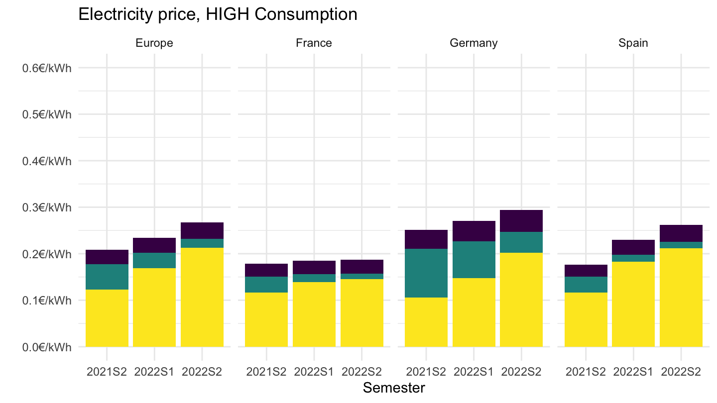

2020-

Code

nrg_pc_204 |>
  filter(geo %in% c("FR", "DE", "EA", "ES"),
         tax %in% c("I_TAX", "X_TAX"),
         nrg_cons == "KWH_GE15000",
         currency == "EUR") |>
  semester_to_date() |>
  filter(date >= as.Date("2020-01-01")) |>
  mutate(Geo = ifelse(geo == "EA", "Europe", Geo)) |>
  add_flag_color("Geo") |>
  ggplot() + geom_line(aes(x = date, y = values, color = color, linetype = Tax)) +
  scale_color_identity() + theme_minimal()  + add_flags +
  scale_x_date(breaks = as.Date(paste0(seq(1960, 2100, 1), "-01-01")),
               labels = date_format("%Y")) +
  theme(legend.position = c(0.2, 0.8),
        legend.title = element_blank()) +
  xlab("") + ylab("Band DE : Consumption > 15 000 kWh") +
  scale_y_log10(breaks = seq(-30, 30, .05),
                labels = dollar_format(a = .01, pre = "", su = "€"))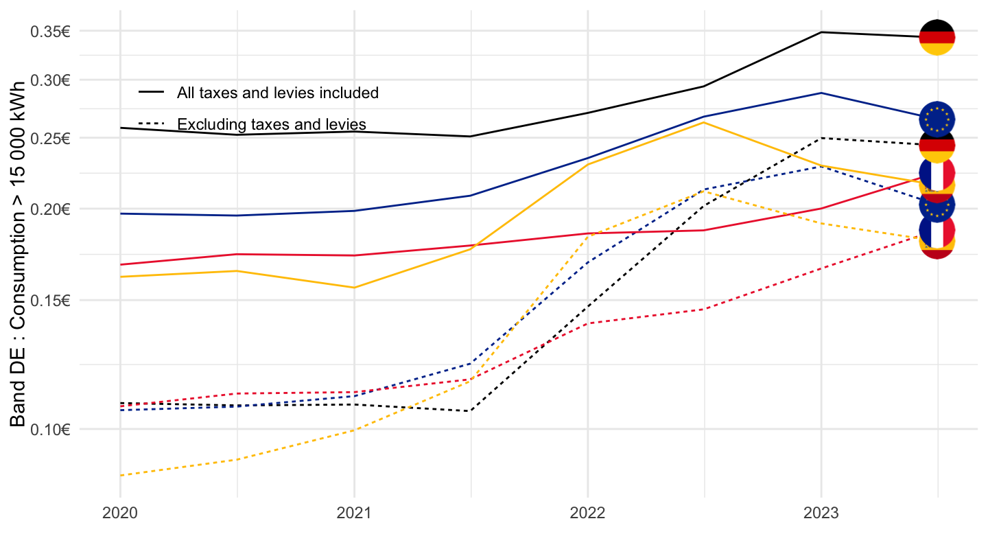

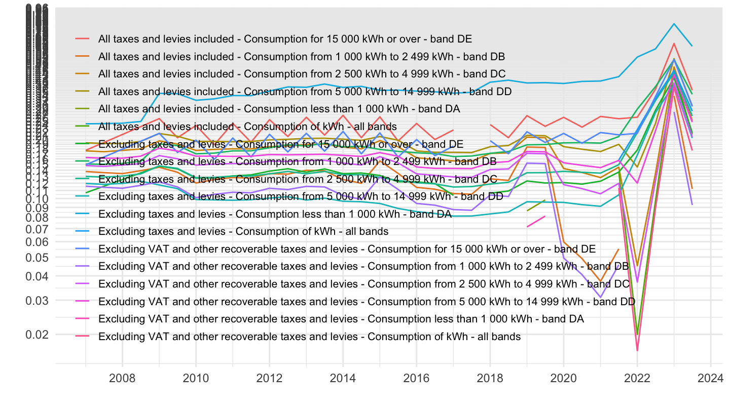
Euros

Euro Area EA

All

Code

nrg_pc_204 |>
  filter(geo == "EA",
         currency == "EUR") |>
  select_if(~ n_distinct(.) > 1) |>
  semester_to_date() |>
  ggplot() + geom_line(aes(x = date, y = values, color = paste0(Tax, " - ", Nrg_cons))) +
  theme_minimal() + xlab("") + ylab("") +
  scale_x_date(breaks = seq(1920, 2100, 2) |> paste0("-01-01") |> as.Date(),
               labels = date_format("%Y")) +
  scale_y_log10(breaks = seq(0, 1, 0.01)) +
  theme(legend.position = c(0.45, 0.5),
        legend.title = element_blank(),
        legend.text = element_text(size = 8),
        legend.key.size = unit(0.9, 'lines'))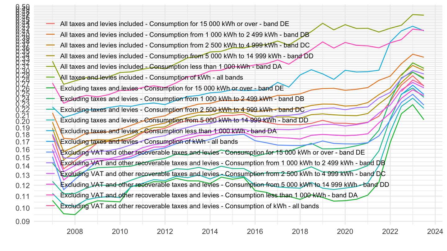

2020-

Code

nrg_pc_204 |>
  filter(geo == "EA",
         currency == "EUR") |>
  select_if(~ n_distinct(.) > 1) |>
  semester_to_date() |>
  filter(date >= as.Date("2020-01-01")) |>
  ggplot() + geom_line(aes(x = date, y = values, color = paste0(Tax, " - ", Nrg_cons))) +
  theme_minimal() + xlab("") + ylab("") +
  scale_x_date(breaks = seq(1920, 2100, 1) |> paste0("-01-01") |> as.Date(),
               labels = date_format("%Y")) +
  scale_y_log10(breaks = seq(0, 1, 0.01)) +
  theme(legend.position = c(0.45, 0.5),
        legend.title = element_blank(),
        legend.text = element_text(size = 8),
        legend.key.size = unit(0.9, 'lines'))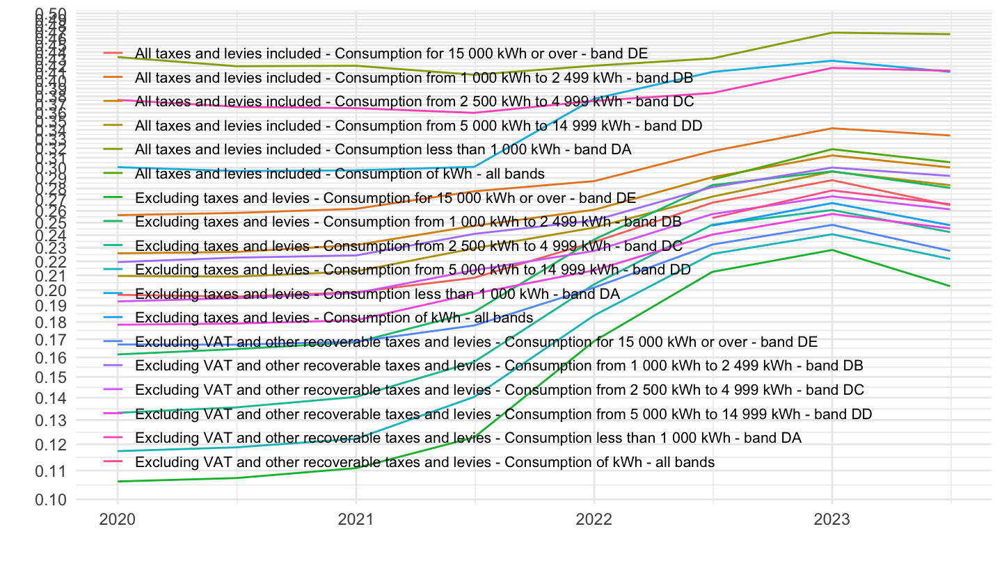

France

All

Code

nrg_pc_204 |>
  filter(geo == "FR",
         currency == "EUR") |>
  select_if(~ n_distinct(.) > 1) |>
  semester_to_date() |>
  ggplot() + geom_line(aes(x = date, y = values, color = Nrg_cons, linetype = Tax)) +
  theme_minimal() + xlab("") + ylab("") +
  scale_x_date(breaks = seq(1920, 2100, 2) |> paste0("-01-01") |> as.Date(),
               labels = date_format("%Y")) +
  scale_y_log10(breaks = seq(0, 1, 0.01)) +
  theme(legend.position = c(0.45, 0.5),
        legend.title = element_blank(),
        legend.text = element_text(size = 8),
        legend.key.size = unit(0.9, 'lines'))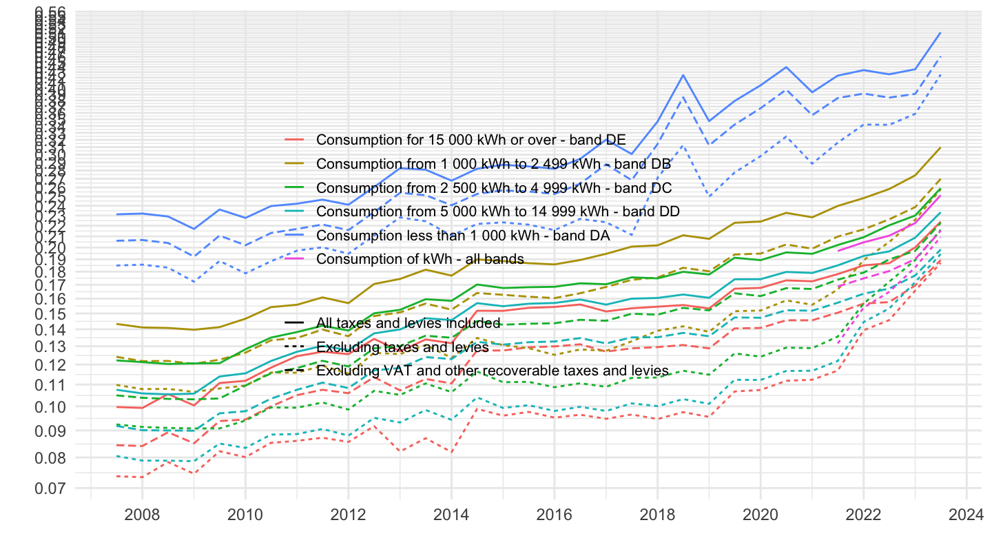

2020-

Code

nrg_pc_204 |>
  filter(geo == "FR",
         currency == "EUR") |>
  select_if(~ n_distinct(.) > 1) |>
  semester_to_date() |>
  filter(date >= as.Date("2020-01-01")) |>
  ggplot() + geom_line(aes(x = date, y = values, color = paste0(Tax, " - ", Nrg_cons))) +
  theme_minimal() + xlab("") + ylab("") +
  scale_x_date(breaks = seq(1920, 2100, 2) |> paste0("-01-01") |> as.Date(),
               labels = date_format("%Y")) +
  scale_y_log10(breaks = seq(0, 1, 0.01)) +
  theme(legend.position = c(0.45, 0.5),
        legend.title = element_blank(),
        legend.text = element_text(size = 8),
        legend.key.size = unit(0.9, 'lines'))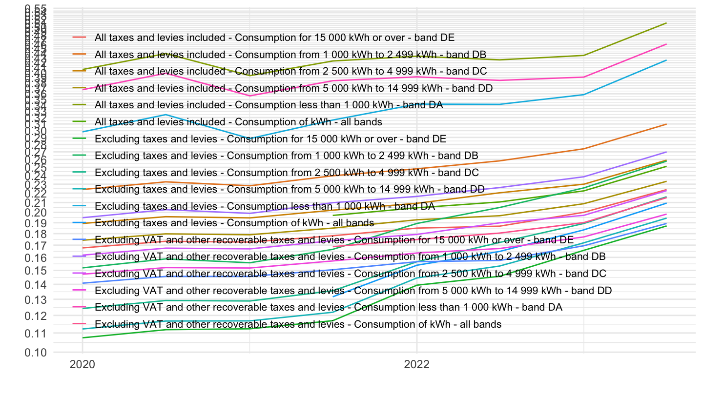

Germany

Code

nrg_pc_204 |>
  filter(geo == "DE",
         unit == "KWH",
         currency == "EUR") |>
  select_if(~ n_distinct(.) > 1) |>
  semester_to_date() |>
  ggplot() + geom_line(aes(x = date, y = values, color = paste0(Tax, " - ", Nrg_cons))) +
  theme_minimal() + xlab("") + ylab("") +
  scale_x_date(breaks = seq(1920, 2100, 2) |> paste0("-01-01") |> as.Date(),
               labels = date_format("%Y")) +
  scale_y_log10(breaks = seq(0, 1, 0.01)) +
  theme(legend.position = c(0.45, 0.5),
        legend.title = element_blank(),
        legend.text = element_text(size = 8),
        legend.key.size = unit(0.9, 'lines'))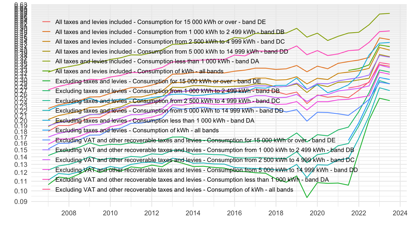

Italy

Code

nrg_pc_204 |>
  filter(geo == "IT",
         unit == "KWH",
         currency == "EUR") |>
  select_if(~ n_distinct(.) > 1) |>
  semester_to_date() |>
  ggplot() + geom_line(aes(x = date, y = values, color = paste0(Tax, " - ", Nrg_cons))) +
  theme_minimal() + xlab("") + ylab("") +
  scale_x_date(breaks = seq(1920, 2100, 2) |> paste0("-01-01") |> as.Date(),
               labels = date_format("%Y")) +
  scale_y_log10(breaks = seq(0, 1, 0.01)) +
  theme(legend.position = c(0.45, 0.5),
        legend.title = element_blank(),
        legend.text = element_text(size = 8),
        legend.key.size = unit(0.9, 'lines'))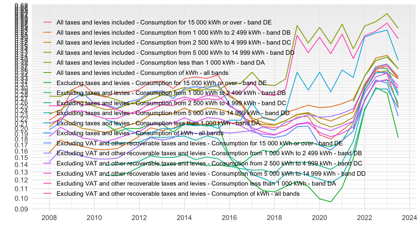

Spain

Code

nrg_pc_204 |>
  filter(geo == "ES",
         currency == "EUR") |>
  select_if(~ n_distinct(.) > 1) |>
  semester_to_date() |>
  ggplot() + geom_line(aes(x = date, y = values, color = paste0(Tax, " - ", Nrg_cons))) +
  theme_minimal() + xlab("") + ylab("") +
  scale_x_date(breaks = seq(1920, 2100, 2) |> paste0("-01-01") |> as.Date(),
               labels = date_format("%Y")) +
  scale_y_log10(breaks = seq(0, 1, 0.01)) +
  theme(legend.position = c(0.45, 0.5),
        legend.title = element_blank(),
        legend.text = element_text(size = 8),
        legend.key.size = unit(0.9, 'lines'))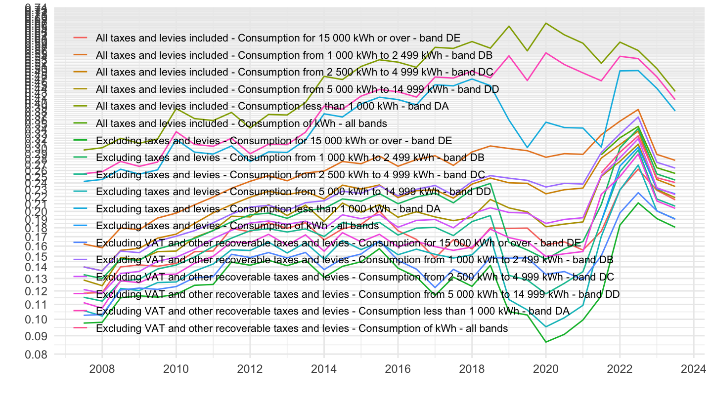

Netherlands

Code

nrg_pc_204 |>
  filter(geo == "NL",
         currency == "EUR") |>
  select_if(~ n_distinct(.) > 1) |>
  semester_to_date() |>
  ggplot() + geom_line(aes(x = date, y = values, color = paste0(Tax, " - ", Nrg_cons))) +
  theme_minimal() + xlab("") + ylab("") +
  scale_x_date(breaks = seq(1920, 2100, 2) |> paste0("-01-01") |> as.Date(),
               labels = date_format("%Y")) +
  scale_y_log10(breaks = seq(0, 1, 0.01)) +
  theme(legend.position = c(0.45, 0.5),
        legend.title = element_blank(),
        legend.text = element_text(size = 8),
        legend.key.size = unit(0.9, 'lines'))

Related Data

Data on energy

source	dataset	Title	Updated
eurostat	nrg_pc_204	Electricity prices for household consumers - bi-annual data (from 2007 onwards) - nrg_pc_204	2026-08-13
ec	WOB	Weekly Oil Bulletin - WOB	2026-09-03
eurostat	ei_isen_m	Energy - monthly data - ei_isen_m	2026-09-03
eurostat	nrg_bal_c	Complete energy balances - nrg_bal_c	2026-08-13
eurostat	nrg_pc_202	Gas prices for household consumers - bi-annual data (from 2007 onwards) - nrg_pc_202	2026-08-11
eurostat	nrg_pc_203	Gas prices for non-household consumers - bi-annual data (from 2007 onwards) - nrg_pc_203	2026-08-10
eurostat	nrg_pc_203_c	Gas prices components for non-household consumers - annual data - nrg_pc_203_c	2026-08-13
eurostat	nrg_pc_203_h	Gas prices for industrial consumers - bi-annual data (until 2007) - nrg_pc_203_h	2026-07-15
eurostat	nrg_pc_203_v	Non-household consumption volumes of gas by consumption bands - nrg_pc_203_v	2026-08-12
eurostat	nrg_pc_205	Electricity prices for non-household consumers - bi-annual data (from 2007 onwards) - nrg_pc_205	2023-06-11
fred	energy	Energy - energy	2026-09-01
iea	world_energy_balances_highlights_2022	World Energy Balances Highlights (2022 edition) - world_energy_balances_highlights_2022	2026-08-01
wb	CMO	World Bank Commodity Price Data (The Pink Sheet) - CMO	2026-09-03
wdi	EG.GDP.PUSE.KO.PP.KD	GDP per unit of energy use (constant 2017 PPP $ per kg of oil equivalent) - EG.GDP.PUSE.KO.PP.KD	2026-09-03
wdi	EG.USE.PCAP.KG.OE	Energy use (kg of oil equivalent per capita) - EG.USE.PCAP.KG.OE	2026-09-03
yahoo	energy	Energy - energy	2026-09-03