Gas prices for household consumers - bi-annual data (from 2007 onwards)
Data - Eurostat
Info
Last observation: Semi-annual: 2025S2 (N = 1,626)
First observation: Semi-annual: 2007S1 (N = 306)
Last data update: 23 jul 2026, 23:02. Last compile: 24 jul 2026, 03:11
Structure
Band D1 : Consumption < 20 GJ
France, Germany, Italy, Spain
All
Code
nrg_pc_202 %>%
  filter(geo %in% c("FR", "DE", "IT", "ES"),
         tax %in% c("I_TAX", "X_TAX"),
         unit == "KWH",
         nrg_cons == "GJ_LT20",
         currency == "EUR") %>%


  semester_to_date %>%
  left_join(colors, by = c("Geo" = "country")) %>%
  ggplot + geom_line(aes(x = date, y = values, color = color, linetype = Tax)) +
  scale_color_identity() + theme_minimal()  + add_8flags +
  scale_x_date(breaks = as.Date(paste0(seq(1960, 2100, 2), "-01-01")),
               labels = date_format("%Y")) +
  theme(legend.position = c(0.2, 0.9),
        legend.title = element_blank()) +
  xlab("") + ylab("Band D1 : Consumption < 20 GJ") +
  scale_y_log10(breaks = seq(0.02, 0.2, 0.01),
                labels = dollar_format(a = .01, pre = "", su = "€"))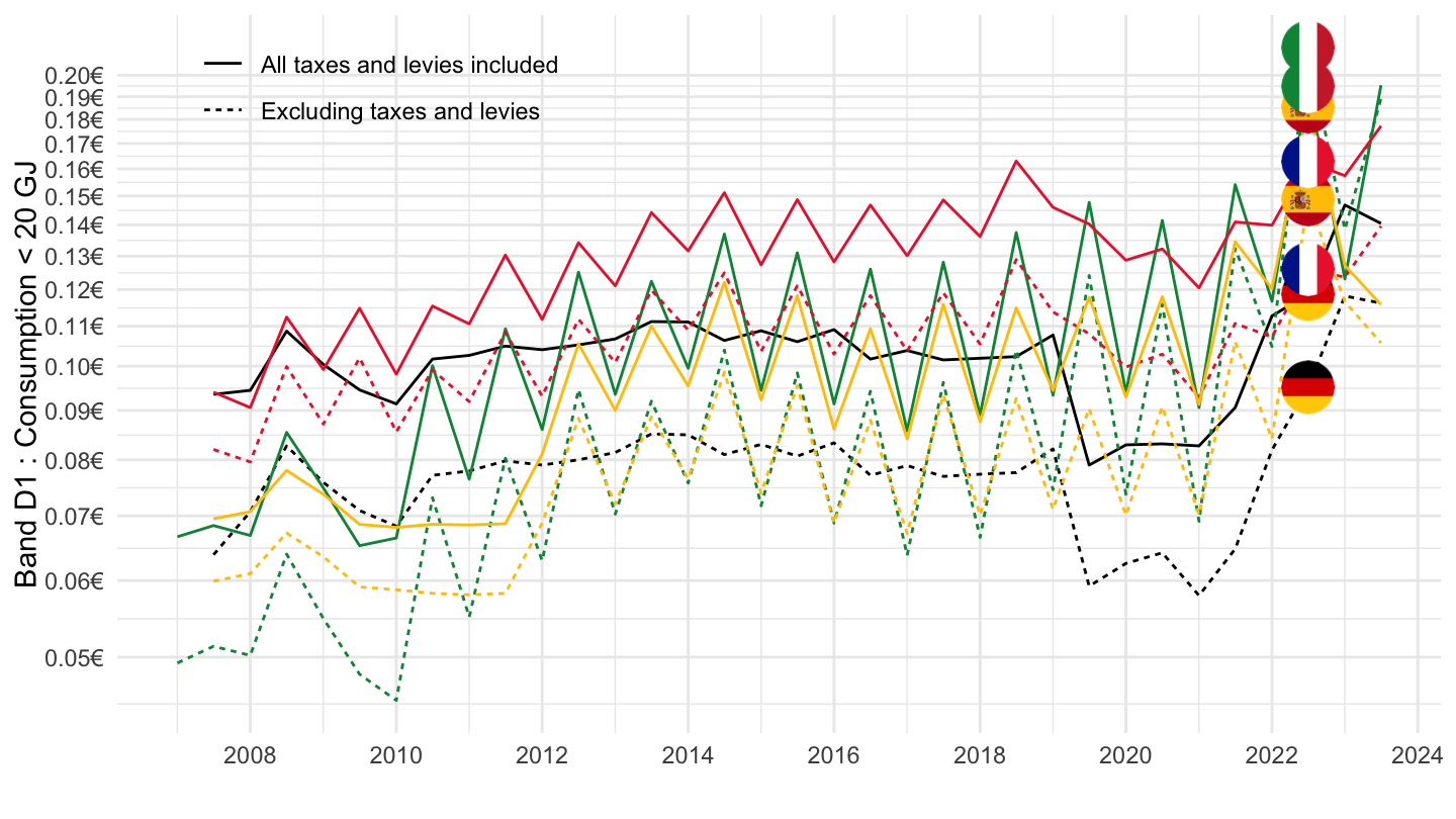
2016-
Code
nrg_pc_202 %>%
  filter(geo %in% c("FR", "DE", "IT", "ES"),
         tax %in% c("I_TAX", "X_TAX"),
         unit == "KWH",
         nrg_cons == "GJ_LT20",
         currency == "EUR") %>%


  semester_to_date %>%
  filter(date >= as.Date("2016-01-01")) %>%
  left_join(colors, by = c("Geo" = "country")) %>%
  ggplot + geom_line(aes(x = date, y = values, color = color, linetype = Tax)) +
  scale_color_identity() + theme_minimal()  + add_8flags +
  scale_x_date(breaks = as.Date(paste0(seq(1960, 2100, 1), "-01-01")),
               labels = date_format("%Y")) +
  theme(legend.position = c(0.2, 0.9),
        legend.title = element_blank()) +
  xlab("") + ylab("Band D1 : Consumption < 20 GJ") +
  scale_y_log10(breaks = seq(0.02, 0.2, 0.01),
                labels = dollar_format(a = .01, pre = "", su = "€"))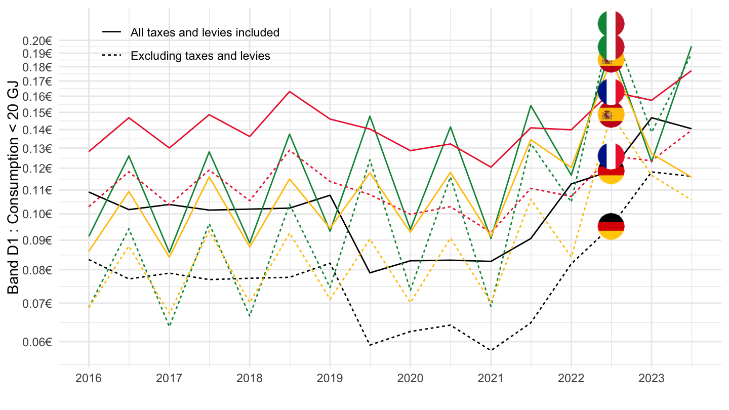
France, Germany, Europe, Spain
Bar
Code
nrg_pc_202 %>%
  filter(geo %in% c("FR", "DE", "EA", "ES"),
         nrg_cons == "GJ_LT20",
         currency == "EUR",
         unit == "KWH",
         time %in% c("2021S2", "2022S1", "2022S2", "2023S1")) %>%
  select_if(~n_distinct(.) > 1) %>%

  mutate(Geo = ifelse(geo == "EA", "Europe", Geo)) %>%
  spread(tax, values) %>%
  transmute(time, Geo,
            ` Taxes except VAT` = X_VAT-X_TAX,
            `  VAT` = I_TAX-X_VAT,
            `Excluding taxes` = X_TAX) %>%
  gather(Tax, values, - time, -Geo) %>%
  ggplot(., aes(x = time, y = values, fill = Tax)) +
  geom_bar(stat = "identity",
           position = "stack") +
  facet_grid(~ Geo) + theme_minimal() +
theme(legend.position = "none",
      legend.title = element_blank()) +
  scale_fill_manual(values = viridis(3)[1:3]) +
  scale_y_continuous(breaks = seq(-30, 30, .05),
                labels = dollar_format(a = .01, pre = "", su = "€/kWh"),
                limits = c(0, 0.2))  +
  xlab("Semester") + ylab("") +
  ggtitle("Natural gas price, LOW Consumption")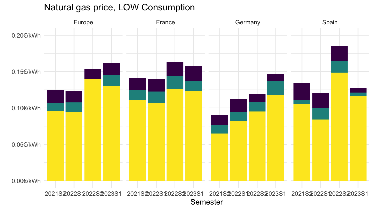
All
Code
nrg_pc_202 %>%
  filter(geo %in% c("FR", "DE", "EA", "ES"),
         tax %in% c("I_TAX", "X_TAX"),
         unit == "KWH",
         nrg_cons == "GJ_LT20",
         currency == "EUR") %>%


  semester_to_date %>%
  mutate(Geo = ifelse(geo == "EA", "Europe", Geo)) %>%
  left_join(colors, by = c("Geo" = "country")) %>%
  ggplot + geom_line(aes(x = date, y = values, color = color, linetype = Tax)) +
  scale_color_identity() + theme_minimal()  + add_8flags +
  scale_x_date(breaks = as.Date(paste0(seq(1960, 2100, 2), "-01-01")),
               labels = date_format("%Y")) +
  theme(legend.position = c(0.2, 0.9),
        legend.title = element_blank()) +
  xlab("") + ylab("Band D1 : Consumption < 20 GJ") +
  scale_y_log10(breaks = seq(0.02, 0.2, 0.01),
                labels = dollar_format(a = .01, pre = "", su = "€"))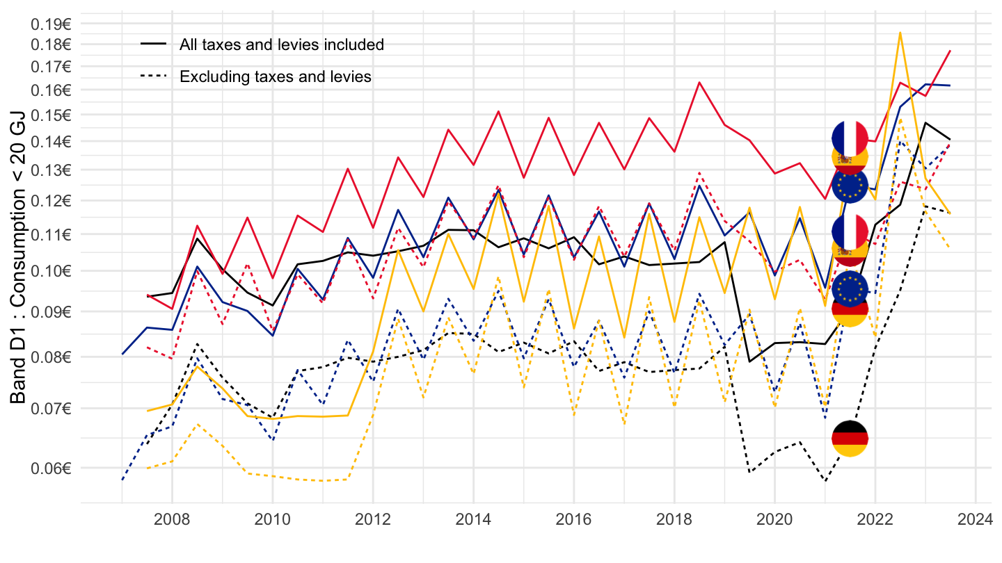
2016-
Code
nrg_pc_202 %>%
  filter(geo %in% c("FR", "DE", "EA", "ES"),
         tax %in% c("I_TAX", "X_TAX"),
         unit == "KWH",
         nrg_cons == "GJ_LT20",
         currency == "EUR") %>%


  semester_to_date %>%
  filter(date >= as.Date("2016-01-01")) %>%
  mutate(Geo = ifelse(geo == "EA", "Europe", Geo)) %>%
  left_join(colors, by = c("Geo" = "country")) %>%
  ggplot + geom_line(aes(x = date, y = values, color = color, linetype = Tax)) +
  scale_color_identity() + theme_minimal()  + add_8flags +
  scale_x_date(breaks = as.Date(paste0(seq(1960, 2100, 1), "-01-01")),
               labels = date_format("%Y")) +
  theme(legend.position = c(0.2, 0.9),
        legend.title = element_blank()) +
  xlab("") + ylab("Band D1 : Consumption < 20 GJ") +
  scale_y_log10(breaks = seq(0.02, 0.2, 0.01),
                labels = dollar_format(a = .01, pre = "", su = "€"))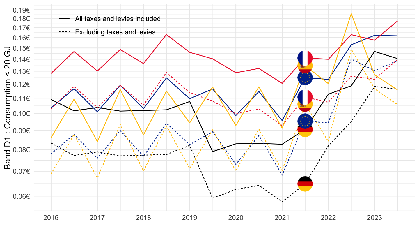
2020-
Code
nrg_pc_202 %>%
  filter(geo %in% c("FR", "DE", "EA", "ES"),
         tax %in% c("I_TAX", "X_TAX"),
         unit == "KWH",
         nrg_cons == "GJ_LT20",
         currency == "EUR") %>%


  semester_to_date %>%
  filter(date >= as.Date("2020-01-01")) %>%
  mutate(Geo = ifelse(geo == "EA", "Europe", Geo)) %>%
  left_join(colors, by = c("Geo" = "country")) %>%
  ggplot + geom_line(aes(x = date, y = values, color = color, linetype = Tax)) +
  scale_color_identity() + theme_minimal()  + add_8flags +
  scale_x_date(breaks = as.Date(paste0(seq(1960, 2100, 1), "-01-01")),
               labels = date_format("%Y")) +
  theme(legend.position = c(0.2, 0.9),
        legend.title = element_blank()) +
  xlab("") + ylab("Band D1 : Consumption < 20 GJ") +
  scale_y_log10(breaks = seq(0.02, 0.2, 0.01),
                labels = dollar_format(a = .01, pre = "", su = "€"))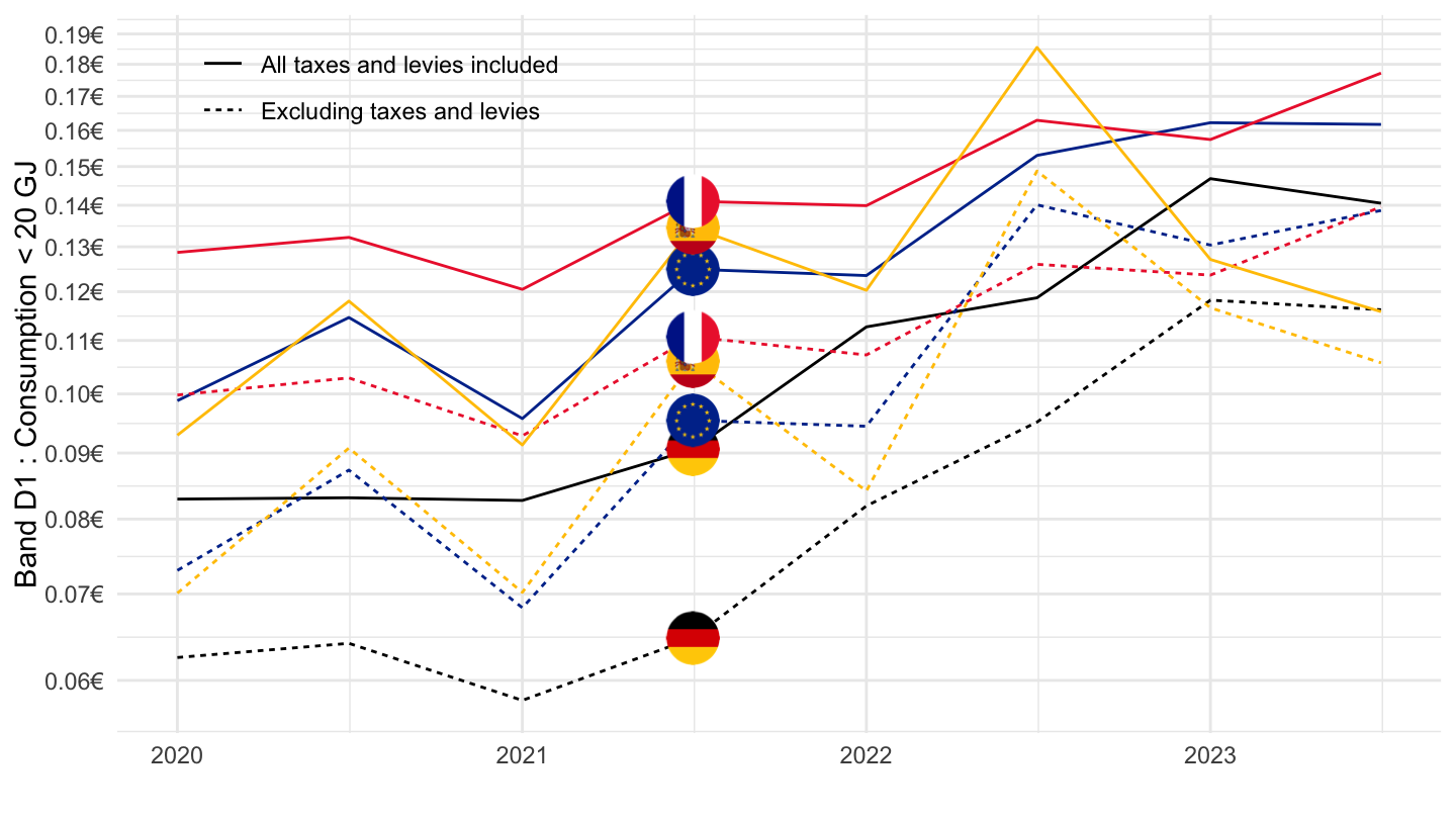
Greece, Belgium, Austria, Portugal
All
Code
nrg_pc_202 %>%
  filter(geo %in% c("EL", "BE", "AT", "PT"),
         tax %in% c("I_TAX", "X_TAX"),
         unit == "KWH",
         nrg_cons == "GJ_LT20",
         currency == "EUR") %>%


  semester_to_date %>%
  left_join(colors, by = c("Geo" = "country")) %>%
  ggplot + geom_line(aes(x = date, y = values, color = color, linetype = Tax)) +
  scale_color_identity() + theme_minimal()  + add_8flags +
  scale_x_date(breaks = as.Date(paste0(seq(1960, 2100, 2), "-01-01")),
               labels = date_format("%Y")) +
  theme(legend.position = c(0.2, 0.9),
        legend.title = element_blank()) +
  xlab("") + ylab("Band D1 : Consumption < 20 GJ") +
  scale_y_log10(breaks = seq(0.02, 0.2, 0.01),
                labels = dollar_format(a = .01, pre = "", su = "€"))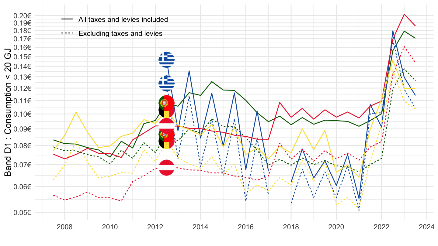
2016-
Code
nrg_pc_202 %>%
  filter(geo %in% c("EL", "BE", "AT", "PT"),
         tax %in% c("I_TAX", "X_TAX"),
         unit == "KWH",
         nrg_cons == "GJ_LT20",
         currency == "EUR") %>%


  semester_to_date %>%
  filter(date >= as.Date("2016-01-01")) %>%
  left_join(colors, by = c("Geo" = "country")) %>%
  ggplot + geom_line(aes(x = date, y = values, color = color, linetype = Tax)) +
  scale_color_identity() + theme_minimal()  + add_8flags +
  scale_x_date(breaks = as.Date(paste0(seq(1960, 2100, 1), "-01-01")),
               labels = date_format("%Y")) +
  theme(legend.position = c(0.2, 0.9),
        legend.title = element_blank()) +
  xlab("") + ylab("Band D1 : Consumption < 20 GJ") +
  scale_y_log10(breaks = seq(0.02, 0.2, 0.01),
                labels = dollar_format(a = .01, pre = "", su = "€"))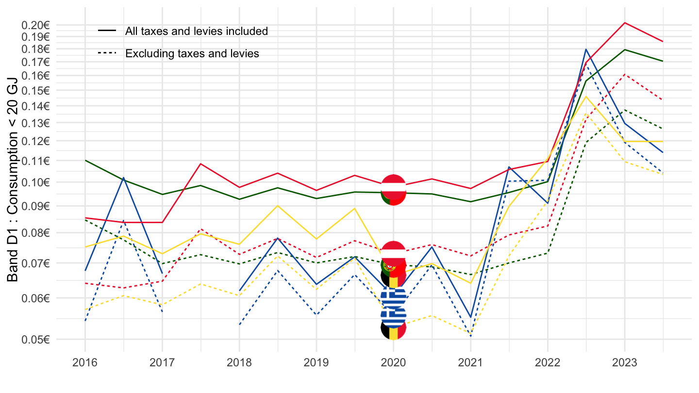
Band D2 : 20 GJ < Consumption < 200 GJ
France, Germany, Italy, Spain
All
Code
nrg_pc_202 %>%
  filter(geo %in% c("FR", "DE", "IT", "ES"),
         tax %in% c("I_TAX", "X_TAX"),
         unit == "KWH",
         nrg_cons == "GJ20-199",
         currency == "EUR") %>%


  semester_to_date %>%
  left_join(colors, by = c("Geo" = "country")) %>%
  ggplot + geom_line(aes(x = date, y = values, color = color, linetype = Tax)) +
  scale_color_identity() + theme_minimal()  + add_8flags +
  scale_x_date(breaks = as.Date(paste0(seq(1960, 2100, 2), "-01-01")),
               labels = date_format("%Y")) +
  theme(legend.position = c(0.2, 0.9),
        legend.title = element_blank()) +
  xlab("") + ylab("20 GJ < Consumption < 200 GJ") +
  scale_y_log10(breaks = seq(0.02, 0.12, 0.01),
                labels = dollar_format(a = .01, pre = "", su = "€"))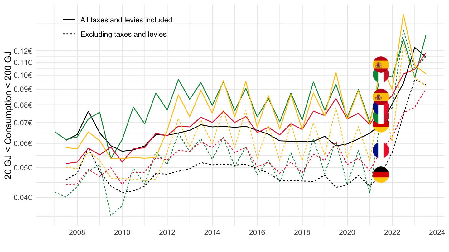
2016-
Code
nrg_pc_202 %>%
  filter(geo %in% c("FR", "DE", "IT", "ES"),
         tax %in% c("I_TAX", "X_TAX"),
         unit == "KWH",
         nrg_cons == "GJ20-199",
         currency == "EUR") %>%


  semester_to_date %>%
  filter(date >= as.Date("2016-01-01")) %>%
  left_join(colors, by = c("Geo" = "country")) %>%
  ggplot + geom_line(aes(x = date, y = values, color = color, linetype = Tax)) +
  scale_color_identity() + theme_minimal()  + add_8flags +
  scale_x_date(breaks = as.Date(paste0(seq(1960, 2100, 1), "-01-01")),
               labels = date_format("%Y")) +
  theme(legend.position = c(0.2, 0.9),
        legend.title = element_blank()) +
  xlab("") + ylab("20 GJ < Consumption < 200 GJ") +
  scale_y_log10(breaks = seq(0.02, 0.12, 0.01),
                labels = dollar_format(a = .01, pre = "", su = "€"))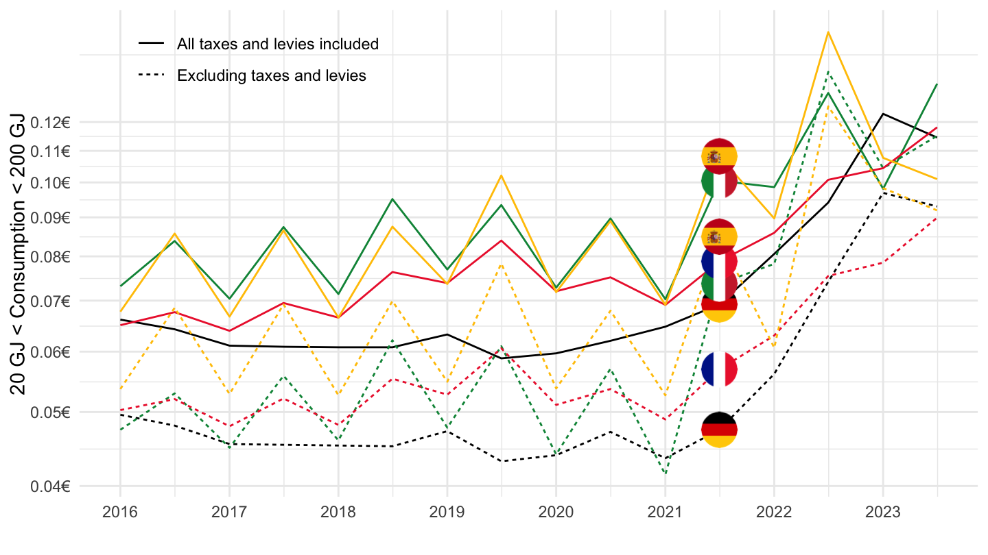
Band D3 : Consumption > 200 GJ
France, Germany, Italy, Spain
All
Code
nrg_pc_202 %>%
  filter(geo %in% c("FR", "DE", "IT", "ES"),
         tax %in% c("I_TAX", "X_TAX"),
         unit == "KWH",
         nrg_cons == "GJ_GE200",
         currency == "EUR") %>%


  semester_to_date %>%
  left_join(colors, by = c("Geo" = "country")) %>%
  ggplot + geom_line(aes(x = date, y = values, color = color, linetype = Tax)) +
  scale_color_identity() + theme_minimal()  + add_8flags +
  scale_x_date(breaks = as.Date(paste0(seq(1960, 2100, 2), "-01-01")),
               labels = date_format("%Y")) +
  theme(legend.position = c(0.2, 0.9),
        legend.title = element_blank()) +
  xlab("") + ylab("Consumption > 200 GJ") +
  scale_y_log10(breaks = seq(0.02, 0.12, 0.01),
                labels = dollar_format(a = .01, pre = "", su = "€"))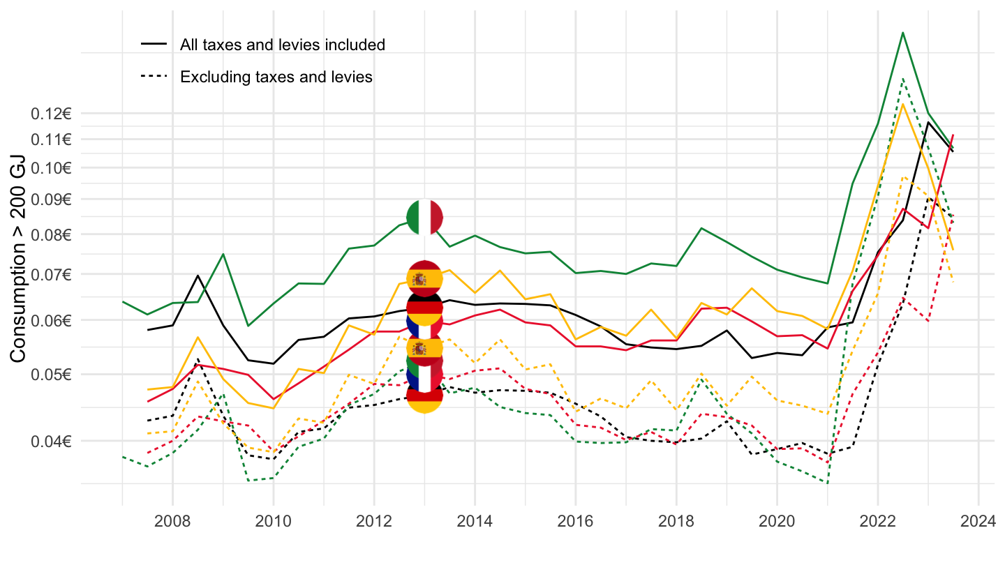
2016-
Code
nrg_pc_202 %>%
  filter(geo %in% c("FR", "DE", "IT", "ES"),
         tax %in% c("I_TAX", "X_TAX"),
         unit == "KWH",
         nrg_cons == "GJ_GE200",
         currency == "EUR") %>%


  semester_to_date %>%
  filter(date >= as.Date("2016-01-01")) %>%
  left_join(colors, by = c("Geo" = "country")) %>%
  ggplot + geom_line(aes(x = date, y = values, color = color, linetype = Tax)) +
  scale_color_identity() + theme_minimal()  + add_8flags +
  scale_x_date(breaks = as.Date(paste0(seq(1960, 2100, 1), "-01-01")),
               labels = date_format("%Y")) +
  theme(legend.position = c(0.2, 0.9),
        legend.title = element_blank()) +
  xlab("") + ylab("Consumption > 200 GJ") +
  scale_y_log10(breaks = seq(0.02, 0.12, 0.01),
                labels = dollar_format(a = .01, pre = "", su = "€"))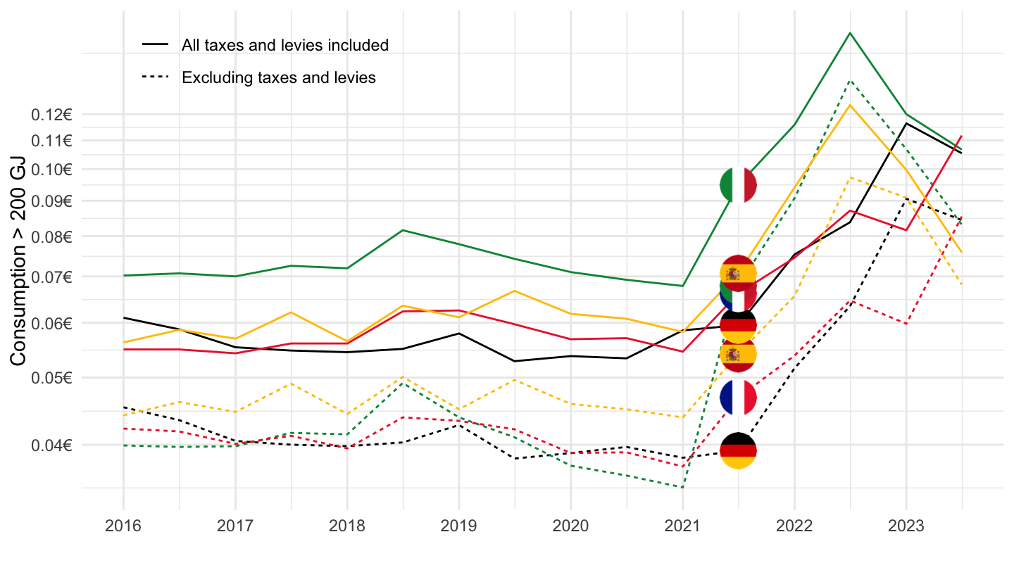
2020-
Code
nrg_pc_202 %>%
  filter(geo %in% c("FR", "DE", "IT", "ES"),
         tax %in% c("I_TAX", "X_TAX"),
         unit == "KWH",
         nrg_cons == "GJ_GE200",
         currency == "EUR") %>%


  semester_to_date %>%
  filter(date >= as.Date("2020-01-01")) %>%
  left_join(colors, by = c("Geo" = "country")) %>%
  ggplot + geom_line(aes(x = date, y = values, color = color, linetype = Tax)) +
  scale_color_identity() + theme_minimal()  + add_8flags +
  scale_x_date(breaks = as.Date(paste0(seq(1960, 2100, 1), "-01-01")),
               labels = date_format("%Y")) +
  theme(legend.position = c(0.2, 0.9),
        legend.title = element_blank()) +
  xlab("") + ylab("Consumption > 200 GJ") +
  scale_y_log10(breaks = seq(0.02, 0.12, 0.01),
                labels = dollar_format(a = .01, pre = "", su = "€"))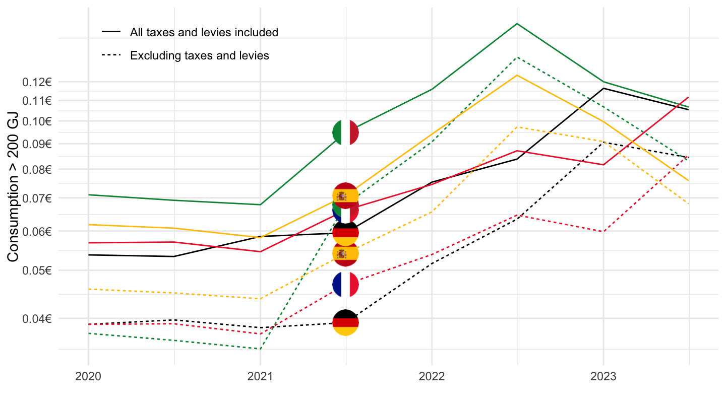
France, Germany, Europe, Spain
Bar
Code
nrg_pc_202 %>%
  filter(geo %in% c("FR", "DE", "EA", "ES"),
         nrg_cons == "GJ_GE200",
         currency == "EUR",
         unit == "KWH",
         time %in% c("2021S2", "2022S1", "2022S2")) %>%
  select_if(~n_distinct(.) > 1) %>%

  mutate(Geo = ifelse(geo == "EA", "Europe", Geo)) %>%
  spread(tax, values) %>%
  transmute(time, Geo,
            ` Taxes except VAT` = X_VAT-X_TAX,
            `  VAT` = I_TAX-X_VAT,
            `Excluding taxes` = X_TAX) %>%
  gather(Tax, values, - time, -Geo) %>%
  ggplot(., aes(x = time, y = values, fill = Tax)) +
  geom_bar(stat = "identity",
           position = "stack") +
  facet_grid(~ Geo) + theme_minimal() +
theme(legend.position = "none",
      legend.title = element_blank()) +
  scale_fill_manual(values = viridis(3)[1:3]) +
  scale_y_continuous(breaks = seq(-30, 30, .05),
                labels = dollar_format(a = .01, pre = "", su = "€/kWh"))  +
  xlab("") + ylab("") +
  ggtitle("Natural gas price, HIGH Consumption")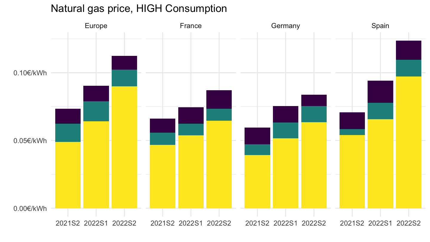
All
Code
nrg_pc_202 %>%
  filter(geo %in% c("FR", "DE", "EA", "ES"),
         tax %in% c("I_TAX", "X_TAX"),
         unit == "KWH",
         nrg_cons == "GJ_GE200",
         currency == "EUR") %>%


  semester_to_date %>%
  mutate(Geo = ifelse(geo == "EA", "Europe", Geo)) %>%
  left_join(colors, by = c("Geo" = "country")) %>%
  ggplot + geom_line(aes(x = date, y = values, color = color, linetype = Tax)) +
  scale_color_identity() + theme_minimal()  + add_8flags +
  scale_x_date(breaks = as.Date(paste0(seq(1960, 2100, 2), "-01-01")),
               labels = date_format("%Y")) +
  theme(legend.position = c(0.2, 0.9),
        legend.title = element_blank()) +
  xlab("") + ylab("Consumption > 200 GJ") +
  scale_y_log10(breaks = seq(0.02, 0.2, 0.01),
                labels = dollar_format(a = .01, pre = "", su = "€"))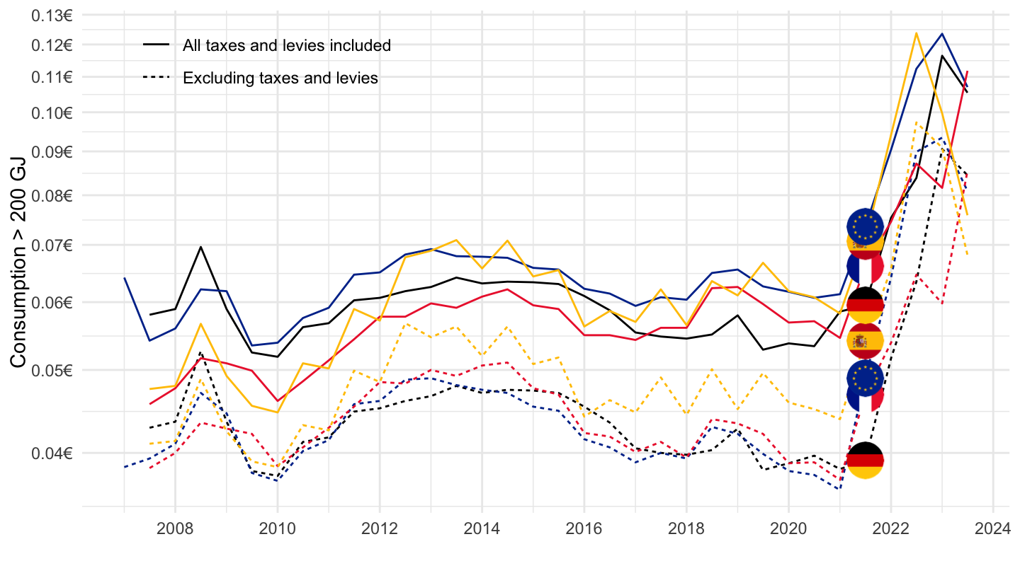
2016-
Code
nrg_pc_202 %>%
  filter(geo %in% c("FR", "DE", "EA", "ES"),
         tax %in% c("I_TAX", "X_TAX"),
         unit == "KWH",
         nrg_cons == "GJ_GE200",
         currency == "EUR") %>%


  semester_to_date %>%
  filter(date >= as.Date("2016-01-01")) %>%
  mutate(Geo = ifelse(geo == "EA", "Europe", Geo)) %>%
  left_join(colors, by = c("Geo" = "country")) %>%
  ggplot + geom_line(aes(x = date, y = values, color = color, linetype = Tax)) +
  scale_color_identity() + theme_minimal()  + add_8flags +
  scale_x_date(breaks = as.Date(paste0(seq(1960, 2100, 1), "-01-01")),
               labels = date_format("%Y")) +
  theme(legend.position = c(0.2, 0.9),
        legend.title = element_blank()) +
  xlab("") + ylab("Consumption > 200 GJ") +
  scale_y_log10(breaks = seq(0.02, 0.2, 0.01),
                labels = dollar_format(a = .01, pre = "", su = "€"))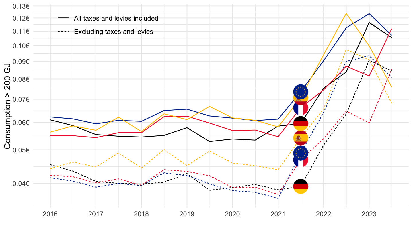
2020-
Code
nrg_pc_202 %>%
  filter(geo %in% c("FR", "DE", "EA", "ES"),
         tax %in% c("I_TAX", "X_TAX"),
         unit == "KWH",
         nrg_cons == "GJ_GE200",
         currency == "EUR") %>%


  semester_to_date %>%
  filter(date >= as.Date("2020-01-01")) %>%
  mutate(Geo = ifelse(geo == "EA", "Europe", Geo)) %>%
  left_join(colors, by = c("Geo" = "country")) %>%
  ggplot + geom_line(aes(x = date, y = values, color = color, linetype = Tax)) +
  scale_color_identity() + theme_minimal()  + add_8flags +
  scale_x_date(breaks = as.Date(paste0(seq(1960, 2100, 1), "-01-01")),
               labels = date_format("%Y")) +
  theme(legend.position = c(0.2, 0.9),
        legend.title = element_blank()) +
  xlab("") + ylab("Consumption > 200 GJ") +
  scale_y_log10(breaks = seq(0.02, 0.2, 0.01),
                labels = dollar_format(a = .01, pre = "", su = "€"))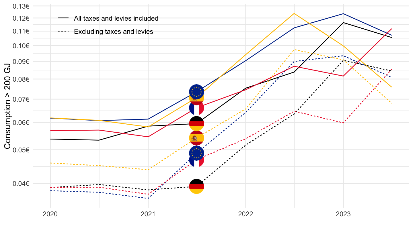
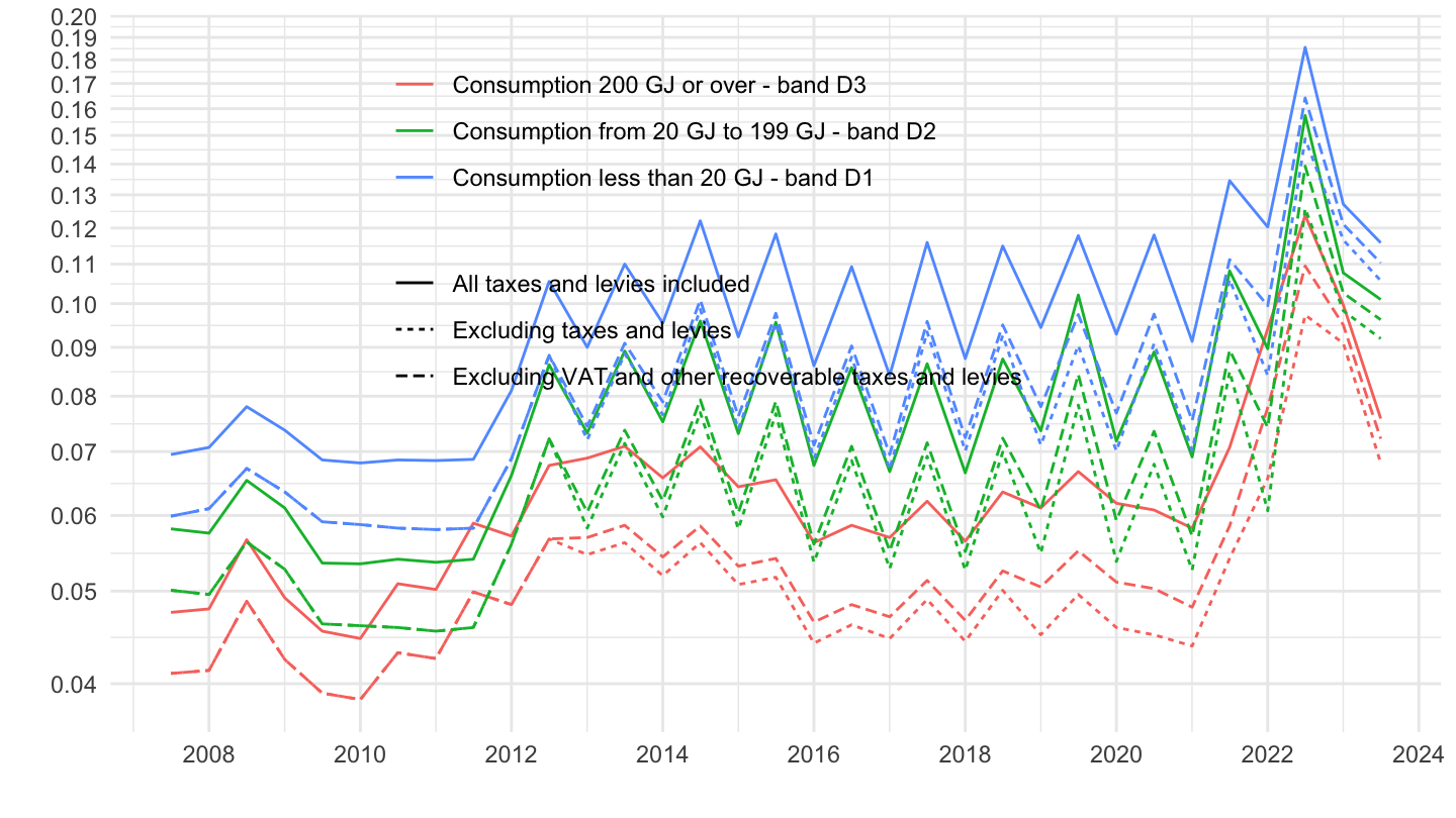
Example
France
Code
nrg_pc_202 %>%
  filter(geo == "FR",
         unit == "KWH",
         currency == "EUR") %>%


  select_if(~ n_distinct(.) > 1) %>%
  semester_to_date %>%
  ggplot + geom_line(aes(x = date, y = values, color = Nrg_cons, linetype = Tax)) +
  theme_minimal() + xlab("") + ylab("") +
  scale_x_date(breaks = seq(1920, 2100, 2) %>% paste0("-01-01") %>% as.Date,
               labels = date_format("%Y")) +
  scale_y_log10(breaks = seq(0, 1, 0.01)) +
  theme(legend.position = c(0.45, 0.7),
        legend.title = element_blank())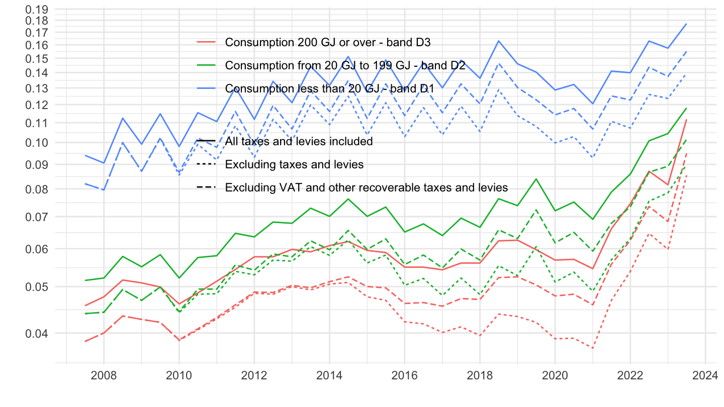
Germany
Code
nrg_pc_202 %>%
  filter(geo == "DE",
         unit == "KWH",
         currency == "EUR") %>%


  select_if(~ n_distinct(.) > 1) %>%
  semester_to_date %>%
  ggplot + geom_line(aes(x = date, y = values, color = Nrg_cons, linetype = Tax)) +
  theme_minimal() + xlab("") + ylab("") +
  scale_x_date(breaks = seq(1920, 2100, 2) %>% paste0("-01-01") %>% as.Date,
               labels = date_format("%Y")) +
  scale_y_log10(breaks = seq(0, 1, 0.01)) +
  theme(legend.position = c(0.45, 0.7),
        legend.title = element_blank())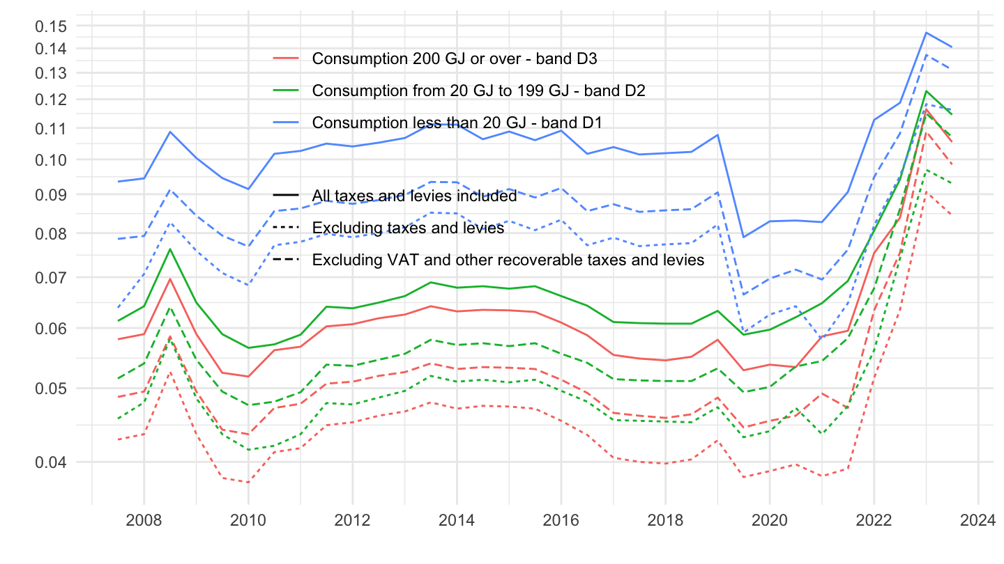
Italy
Code
nrg_pc_202 %>%
  filter(geo == "IT",
         unit == "KWH",
         currency == "EUR") %>%


  select_if(~ n_distinct(.) > 1) %>%
  semester_to_date %>%
  ggplot + geom_line(aes(x = date, y = values, color = Nrg_cons, linetype = Tax)) +
  theme_minimal() + xlab("") + ylab("") +
  scale_x_date(breaks = seq(1920, 2100, 2) %>% paste0("-01-01") %>% as.Date,
               labels = date_format("%Y")) +
  scale_y_log10(breaks = seq(0, 1, 0.01)) +
  theme(legend.position = c(0.45, 0.7),
        legend.title = element_blank())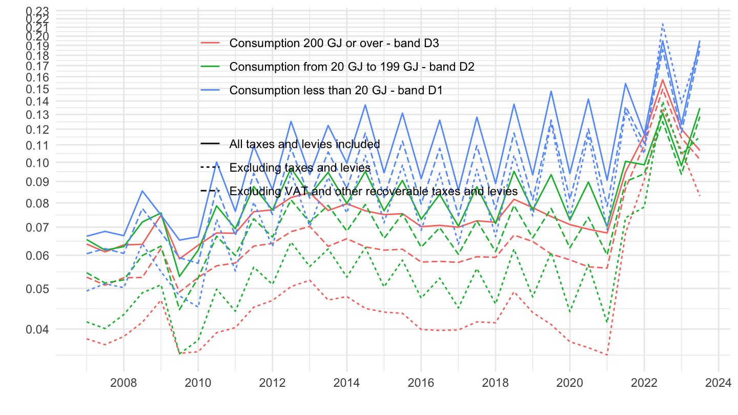
Spain
Code
nrg_pc_202 %>%
  filter(geo == "ES",
         unit == "KWH",
         currency == "EUR") %>%


  select_if(~ n_distinct(.) > 1) %>%
  semester_to_date %>%
  ggplot + geom_line(aes(x = date, y = values, color = Nrg_cons, linetype = Tax)) +
  theme_minimal() + xlab("") + ylab("") +
  scale_x_date(breaks = seq(1920, 2100, 2) %>% paste0("-01-01") %>% as.Date,
               labels = date_format("%Y")) +
  scale_y_log10(breaks = seq(0, 1, 0.01)) +
  theme(legend.position = c(0.45, 0.7),
        legend.title = element_blank())