Gas prices for non-household consumers - bi-annual data (from 2007 onwards)

Data - Eurostat

~/data/eurostat/

Info

Related energy datasets

source	dataset	Title	Download	Compile
eurostat	nrg_pc_203	Gas prices for non-household consumers - bi-annual data (from 2007 onwards)	2023-06-11	2023-06-11
ec	WOB	Weekly Oil Bulletin	2023-06-01	2023-06-01
eurostat	ei_isen_m	Energy - monthly data	2023-06-04	2023-05-04
eurostat	nrg_bal_c	Complete energy balances	2023-06-04	2023-04-16
eurostat	nrg_pc_202	Gas prices for household consumers - bi-annual data (from 2007 onwards)	2023-06-08	2023-06-08
eurostat	nrg_pc_204	Electricity prices for household consumers - bi-annual data (from 2007 onwards)	2023-06-08	2023-06-08
eurostat	nrg_pc_205	Electricity prices for non-household consumers - bi-annual data (from 2007 onwards)	2023-06-11	NA
fred	energy	Energy	2023-06-01	2023-06-02
iea	world_energy_balances_highlights_2022	World Energy Balances Highlights (2022 edition)	2023-04-24	2023-04-24
wdi	EG.GDP.PUSE.KO.PP.KD	GDP per unit of energy use (constant 2017 PPP $ per kg of oil equivalent)	2023-04-26	2022-09-27
wdi	EG.USE.PCAP.KG.OE	Energy use (kg of oil equivalent per capita)	2023-04-26	2022-09-27
yahoo	energy	Energy	2023-05-31	2023-04-26

LAST_COMPILE

LAST_COMPILE
2023-06-11

Last

nrg_pc_203 %>%
  group_by(time) %>%
  summarise(Nobs = n()) %>%
  arrange(desc(time)) %>%
  head(2) %>%
  print_table_conditional()

time	Nobs
2022S2	3444
2022S1	3648

Info

• Electricity and gas prices in the first half of 2022. html / png

consom

nrg_pc_203 %>%
  left_join(consom, by = "consom") %>%
  group_by(consom, Consom) %>%
  summarise(Nobs = n()) %>%
  print_table_conditional()

consom	Consom	Nobs
4142901	Band I1 : Consumption < 1 000 GJ	16932
4142902	Band I2 : 1 000 GJ < Consumption < 10 000 GJ	17112
4142903	Band I3 : 10 000 GJ < Consumption < 100 000 GJ	17544
4142904	Band I4 : 100 000 GJ < Consumption < 1 000 000 GJ	17160
4142905	Band I5 : 1 000 000 GJ < Consumption < 4 000 000 GJ	15006
4142906	Band I6 : Consumption > 4 000 000 GJ	6882
TOT_GJ	Consumption of GJ - all bands	1098

currency

nrg_pc_203 %>%
  left_join(currency, by = "currency") %>%
  group_by(currency, Currency) %>%
  summarise(Nobs = n()) %>%
  arrange(-Nobs) %>%
  print_table_conditional()

currency	Currency	Nobs
EUR	Euro	31854
NAC	National currency	30108
PPS	Purchasing Power Standard	29772

tax

nrg_pc_203 %>%
  left_join(tax, by = "tax") %>%
  group_by(tax, Tax) %>%
  summarise(Nobs = n()) %>%
  arrange(-Nobs) %>%
  print_table_conditional()

tax	Tax	Nobs
I_TAX	All taxes and levies included	30578
X_TAX	Excluding taxes and levies	30578
X_VAT	Excluding VAT and other recoverable taxes and levies	30578

unit

nrg_pc_203 %>%
  left_join(unit, by = "unit") %>%
  group_by(unit, Unit) %>%
  summarise(Nobs = n()) %>%
  arrange(-Nobs) %>%
  print_table_conditional()

unit	Unit	Nobs
GJ_GCV	Gigajoule (gross calorific value - GCV)	45867
KWH	Kilowatt-hour	45867

geo

nrg_pc_203 %>%
  left_join(geo, by = "geo") %>%
  group_by(geo, Geo) %>%
  summarise(Nobs = n()) %>%
  arrange(-Nobs) %>%
  mutate(Geo = ifelse(geo == "DE", "Germany", Geo)) %>%
  mutate(Flag = gsub(" ", "-", str_to_lower(Geo)),
         Flag = paste0('<img src="../../bib/flags/vsmall/', Flag, '.png" alt="Flag">')) %>%
  select(Flag, everything()) %>%
  {if (is_html_output()) datatable(., filter = 'top', rownames = F, escape = F) else .}

time

nrg_pc_203 %>%
  group_by(time) %>%
  summarise(Nobs = n()) %>%
  arrange(desc(time)) %>%
  print_table_conditional()

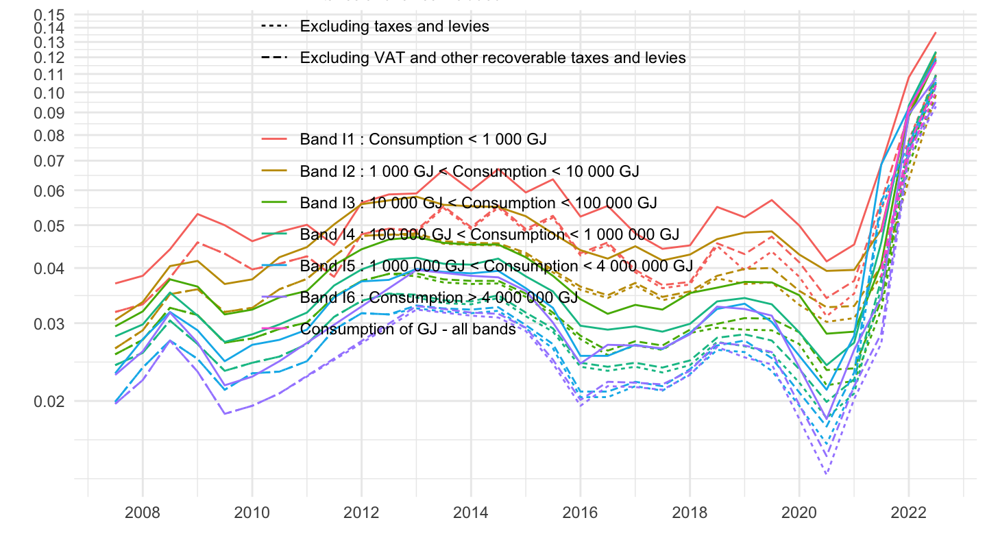
Band I1 : Consumption < 1 000 GJ

France, Germany, Italy, Spain

All

nrg_pc_203 %>%
  filter(geo %in% c("FR", "DE", "IT", "ES"),
         tax %in% c("I_TAX", "X_TAX"),
         unit == "KWH",
         consom == "4142901",
         currency == "EUR") %>%
  left_join(geo, by = "geo") %>%
  left_join(tax, by = "tax") %>%
  semester_to_date %>%
  left_join(colors, by = c("Geo" = "country")) %>%
  ggplot + geom_line(aes(x = date, y = values, color = color, linetype = Tax)) +
  scale_color_identity() + theme_minimal()  + add_8flags +
  scale_x_date(breaks = as.Date(paste0(seq(1960, 2025, 2), "-01-01")),
               labels = date_format("%Y")) +
  theme(legend.position = c(0.2, 0.9),
        legend.title = element_blank()) +
  xlab("") + ylab("Consumption < 1 000 GJ") +
  scale_y_log10(breaks = seq(0.02, 0.2, 0.01),
                labels = dollar_format(a = .01, pre = "", su = "€"))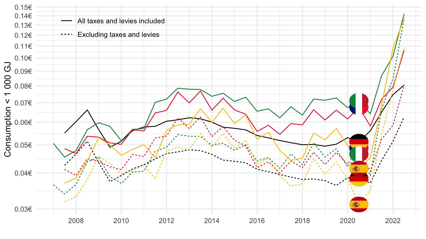

2016-

nrg_pc_203 %>%
  filter(geo %in% c("FR", "DE", "IT", "ES"),
         tax %in% c("I_TAX", "X_TAX"),
         unit == "KWH",
         consom == "4142901",
         currency == "EUR") %>%
  left_join(geo, by = "geo") %>%
  left_join(tax, by = "tax") %>%
  semester_to_date %>%
  filter(date >= as.Date("2016-01-01")) %>%
  left_join(colors, by = c("Geo" = "country")) %>%
  ggplot + geom_line(aes(x = date, y = values, color = color, linetype = Tax)) +
  scale_color_identity() + theme_minimal()  + add_8flags +
  scale_x_date(breaks = as.Date(paste0(seq(1960, 2025, 1), "-01-01")),
               labels = date_format("%Y")) +
  theme(legend.position = c(0.2, 0.9),
        legend.title = element_blank()) +
  xlab("") + ylab("Consumption < 1 000 GJ") +
  scale_y_log10(breaks = seq(0.02, 0.2, 0.01),
                labels = dollar_format(a = .01, pre = "", su = "€"))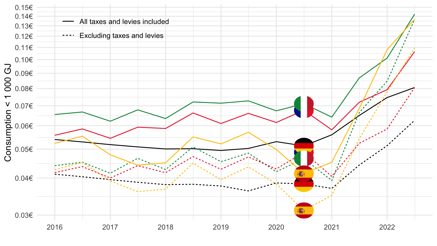

France, Germany, Europe, Spain

Bar

nrg_pc_203 %>%
  filter(geo %in% c("FR", "DE", "EA", "ES"),
         consom == "4142901",
         currency == "EUR",
         unit == "KWH",
         time %in% c("2020S2", "2021S1", "2021S2", "2022S1", "2022S2")) %>%
  select_if(~n_distinct(.) > 1) %>%
  left_join(geo, by = "geo") %>%
  mutate(Geo = ifelse(geo == "EA", "Europe", Geo)) %>%
  spread(tax, values) %>%
  transmute(time, Geo,
            ` Taxes except VAT` = X_VAT-X_TAX,
            `  VAT` = I_TAX-X_VAT,
            `Excluding taxes` = X_TAX) %>%
  gather(Tax, values, - time, -Geo) %>%
  ggplot(., aes(x = time, y = values, fill = Tax)) + 
  geom_bar(stat = "identity",
           position = "stack") +
  facet_grid(~ Geo) + theme_minimal() +
theme(legend.position = "none",
        axis.text.x = element_text(angle = 45, vjust = 1, hjust = 1),
      legend.title = element_blank()) +
  scale_fill_manual(values = viridis(3)[1:3]) +
  scale_y_continuous(breaks = seq(-30, 30, .05),
                labels = dollar_format(a = .01, pre = "", su = "€/kWh"),
                limits = c(0, 0.2))  +
  xlab("Semester") + ylab("") +
  ggtitle("Natural gas price, LOW Consumption")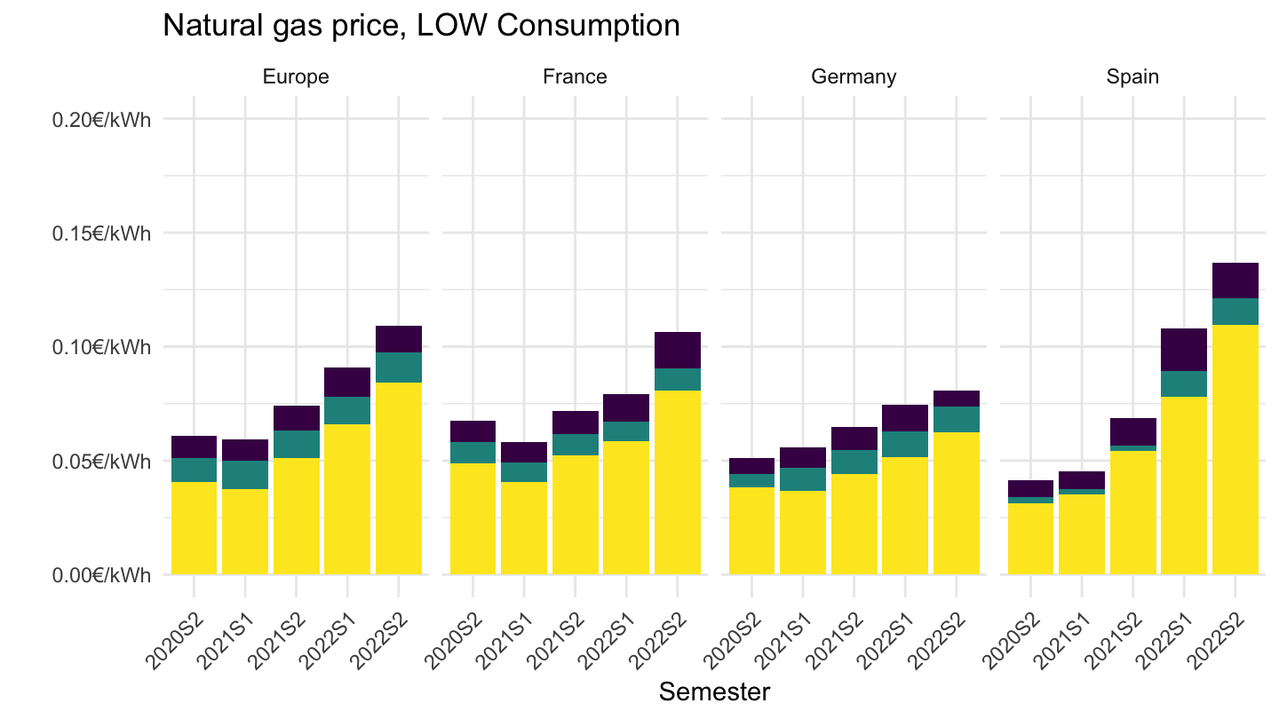

All

nrg_pc_203 %>%
  filter(geo %in% c("FR", "DE", "EA", "ES"),
         tax %in% c("I_TAX", "X_TAX"),
         unit == "KWH",
         consom == "4142901",
         currency == "EUR") %>%
  left_join(geo, by = "geo") %>%
  left_join(tax, by = "tax") %>%
  semester_to_date %>%
  mutate(Geo = ifelse(geo == "EA", "Europe", Geo)) %>%
  left_join(colors, by = c("Geo" = "country")) %>%
  ggplot + geom_line(aes(x = date, y = values, color = color, linetype = Tax)) +
  scale_color_identity() + theme_minimal()  + add_8flags +
  scale_x_date(breaks = as.Date(paste0(seq(1960, 2025, 2), "-01-01")),
               labels = date_format("%Y")) +
  theme(legend.position = c(0.2, 0.9),
        legend.title = element_blank()) +
  xlab("") + ylab("Consumption < 1 000 GJ") +
  scale_y_log10(breaks = seq(0.02, 0.2, 0.01),
                labels = dollar_format(a = .01, pre = "", su = "€"))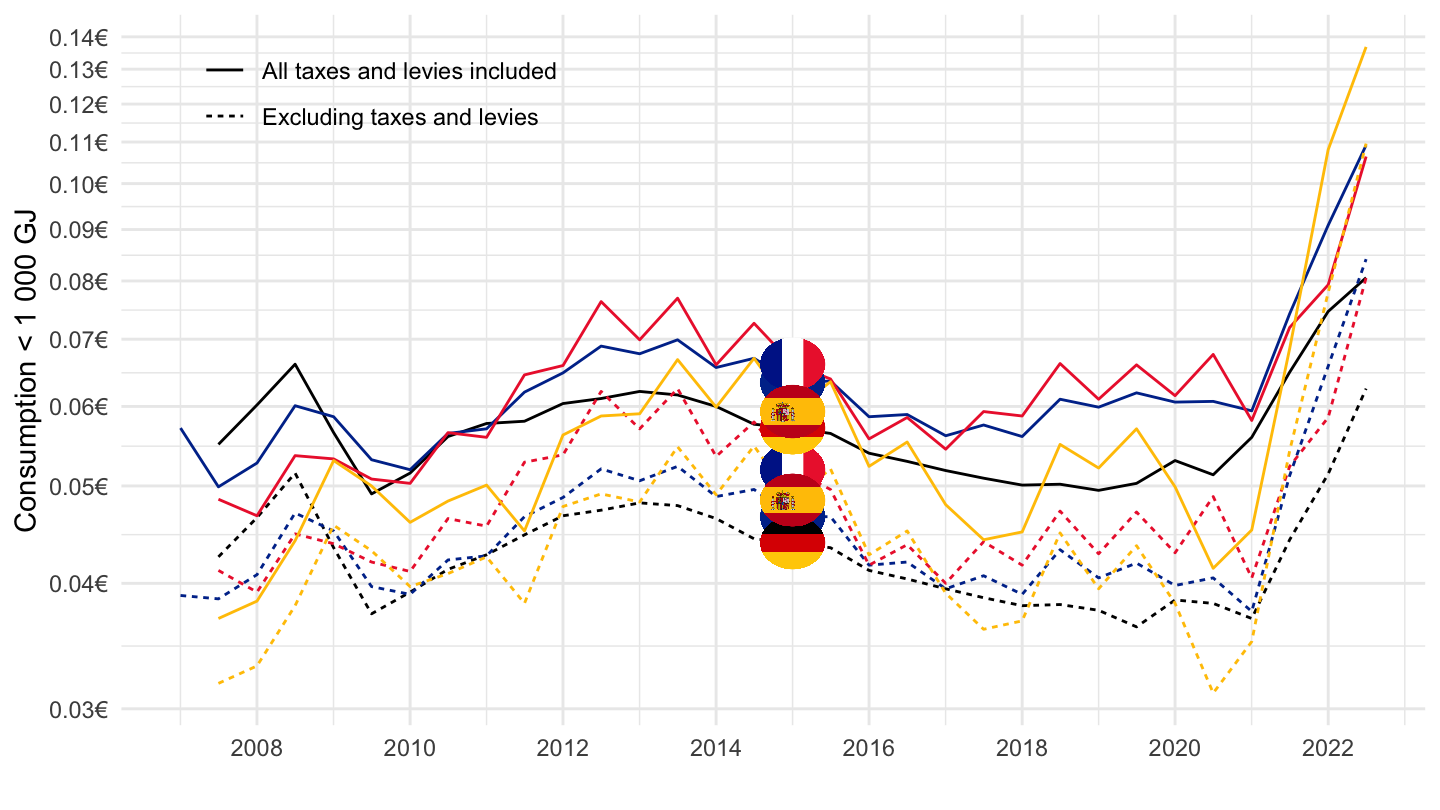

2016-

nrg_pc_203 %>%
  filter(geo %in% c("FR", "DE", "EA", "ES"),
         tax %in% c("I_TAX", "X_TAX"),
         unit == "KWH",
         consom == "4142901",
         currency == "EUR") %>%
  left_join(geo, by = "geo") %>%
  left_join(tax, by = "tax") %>%
  semester_to_date %>%
  filter(date >= as.Date("2016-01-01")) %>%
  mutate(Geo = ifelse(geo == "EA", "Europe", Geo)) %>%
  left_join(colors, by = c("Geo" = "country")) %>%
  ggplot + geom_line(aes(x = date, y = values, color = color, linetype = Tax)) +
  scale_color_identity() + theme_minimal()  + add_8flags +
  scale_x_date(breaks = as.Date(paste0(seq(1960, 2025, 1), "-01-01")),
               labels = date_format("%Y")) +
  theme(legend.position = c(0.2, 0.9),
        legend.title = element_blank()) +
  xlab("") + ylab("Consumption < 1 000 GJ") +
  scale_y_log10(breaks = seq(0.02, 0.2, 0.01),
                labels = dollar_format(a = .01, pre = "", su = "€"))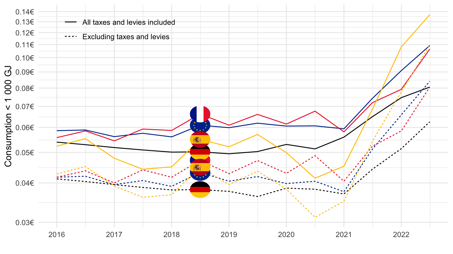

2020-

nrg_pc_203 %>%
  filter(geo %in% c("FR", "DE", "EA", "ES"),
         tax %in% c("I_TAX", "X_TAX"),
         unit == "KWH",
         consom == "4142901",
         currency == "EUR") %>%
  left_join(geo, by = "geo") %>%
  left_join(tax, by = "tax") %>%
  semester_to_date %>%
  filter(date >= as.Date("2020-01-01")) %>%
  mutate(Geo = ifelse(geo == "EA", "Europe", Geo)) %>%
  left_join(colors, by = c("Geo" = "country")) %>%
  ggplot + geom_line(aes(x = date, y = values, color = color, linetype = Tax)) +
  scale_color_identity() + theme_minimal()  + add_8flags +
  scale_x_date(breaks = as.Date(paste0(seq(1960, 2025, 1), "-01-01")),
               labels = date_format("%Y")) +
  theme(legend.position = c(0.2, 0.9),
        legend.title = element_blank()) +
  xlab("") + ylab("Consumption < 1 000 GJ") +
  scale_y_log10(breaks = seq(0.02, 0.2, 0.01),
                labels = dollar_format(a = .01, pre = "", su = "€"))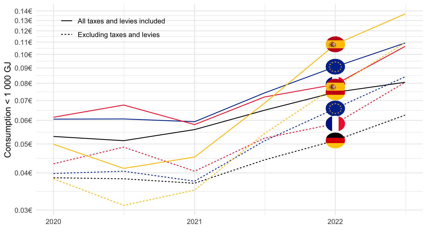

Greece, Belgium, Austria, Portugal

All

nrg_pc_203 %>%
  filter(geo %in% c("EL", "BE", "AT", "PT"),
         tax %in% c("I_TAX", "X_TAX"),
         unit == "KWH",
         consom == "4142901",
         currency == "EUR") %>%
  left_join(geo, by = "geo") %>%
  left_join(tax, by = "tax") %>%
  semester_to_date %>%
  left_join(colors, by = c("Geo" = "country")) %>%
  ggplot + geom_line(aes(x = date, y = values, color = color, linetype = Tax)) +
  scale_color_identity() + theme_minimal()  + add_8flags +
  scale_x_date(breaks = as.Date(paste0(seq(1960, 2025, 2), "-01-01")),
               labels = date_format("%Y")) +
  theme(legend.position = c(0.2, 0.9),
        legend.title = element_blank()) +
  xlab("") + ylab("Consumption < 1 000 GJ") +
  scale_y_log10(breaks = seq(0.02, 0.2, 0.01),
                labels = dollar_format(a = .01, pre = "", su = "€"))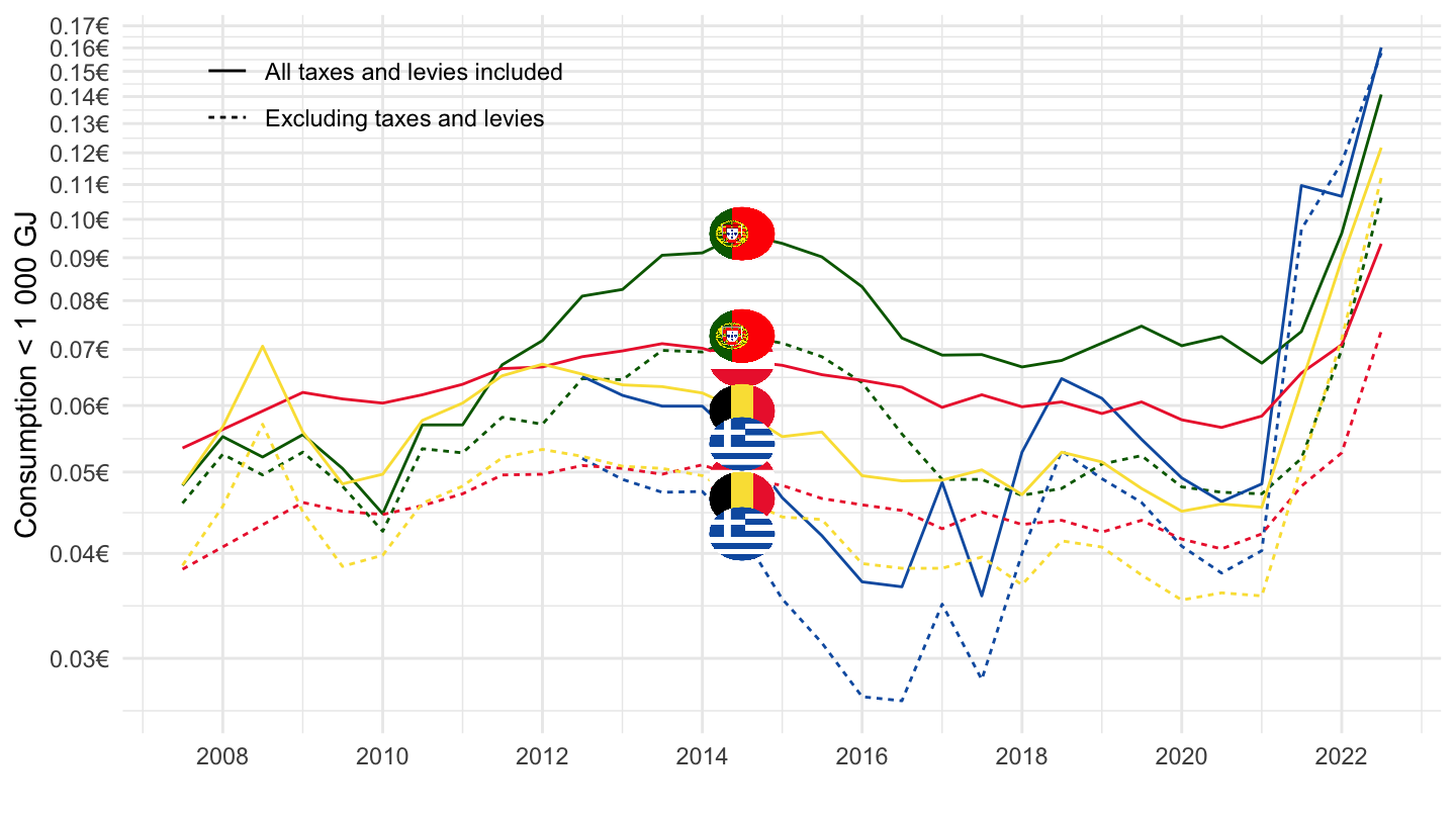

2016-

nrg_pc_203 %>%
  filter(geo %in% c("EL", "BE", "AT", "PT"),
         tax %in% c("I_TAX", "X_TAX"),
         unit == "KWH",
         consom == "4142901",
         currency == "EUR") %>%
  left_join(geo, by = "geo") %>%
  left_join(tax, by = "tax") %>%
  semester_to_date %>%
  filter(date >= as.Date("2016-01-01")) %>%
  left_join(colors, by = c("Geo" = "country")) %>%
  ggplot + geom_line(aes(x = date, y = values, color = color, linetype = Tax)) +
  scale_color_identity() + theme_minimal()  + add_8flags +
  scale_x_date(breaks = as.Date(paste0(seq(1960, 2025, 1), "-01-01")),
               labels = date_format("%Y")) +
  theme(legend.position = c(0.2, 0.9),
        legend.title = element_blank()) +
  xlab("") + ylab("Consumption < 1 000 GJ") +
  scale_y_log10(breaks = seq(0.02, 0.2, 0.01),
                labels = dollar_format(a = .01, pre = "", su = "€"))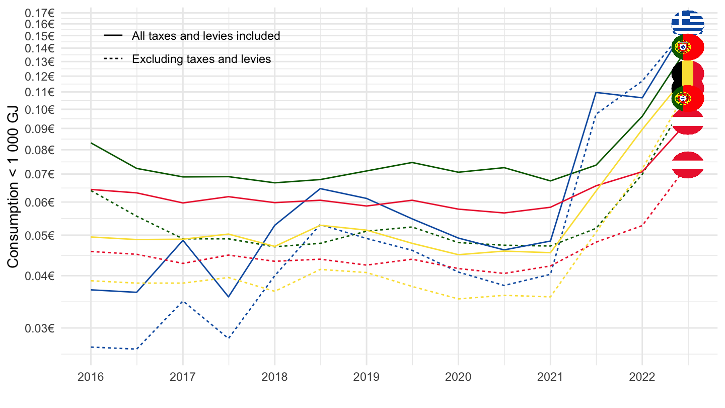

Band I3 : 10 000 GJ < Consumption < 100 000 GJ

France, Germany, Italy, Spain

All

nrg_pc_203 %>%
  filter(geo %in% c("FR", "DE", "IT", "ES"),
         tax %in% c("I_TAX", "X_TAX"),
         unit == "KWH",
         consom == "4142903",
         currency == "EUR") %>%
  left_join(geo, by = "geo") %>%
  left_join(tax, by = "tax") %>%
  semester_to_date %>%
  left_join(colors, by = c("Geo" = "country")) %>%
  ggplot + geom_line(aes(x = date, y = values, color = color, linetype = Tax)) +
  scale_color_identity() + theme_minimal()  + add_8flags +
  scale_x_date(breaks = as.Date(paste0(seq(1960, 2025, 2), "-01-01")),
               labels = date_format("%Y")) +
  theme(legend.position = c(0.2, 0.9),
        legend.title = element_blank()) +
  xlab("") + ylab("Band I3 : 10 000 GJ < Consumption < 100 000 GJ") +
  scale_y_log10(breaks = seq(0.02, 0.12, 0.01),
                labels = dollar_format(a = .01, pre = "", su = "€"))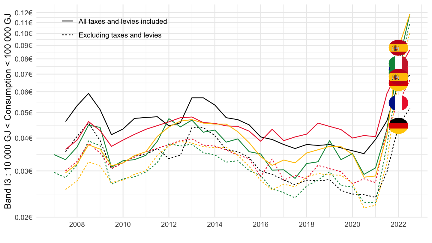

2016-

nrg_pc_203 %>%
  filter(geo %in% c("FR", "DE", "IT", "ES"),
         tax %in% c("I_TAX", "X_TAX"),
         unit == "KWH",
         consom == "4142903",
         currency == "EUR") %>%
  left_join(geo, by = "geo") %>%
  left_join(tax, by = "tax") %>%
  semester_to_date %>%
  filter(date >= as.Date("2016-01-01")) %>%
  left_join(colors, by = c("Geo" = "country")) %>%
  ggplot + geom_line(aes(x = date, y = values, color = color, linetype = Tax)) +
  scale_color_identity() + theme_minimal()  + add_8flags +
  scale_x_date(breaks = as.Date(paste0(seq(1960, 2025, 1), "-01-01")),
               labels = date_format("%Y")) +
  theme(legend.position = c(0.2, 0.9),
        legend.title = element_blank()) +
  xlab("") + ylab("Band I3 : 10 000 GJ < Consumption < 100 000 GJ") +
  scale_y_log10(breaks = seq(0.02, 0.12, 0.01),
                labels = dollar_format(a = .01, pre = "", su = "€"))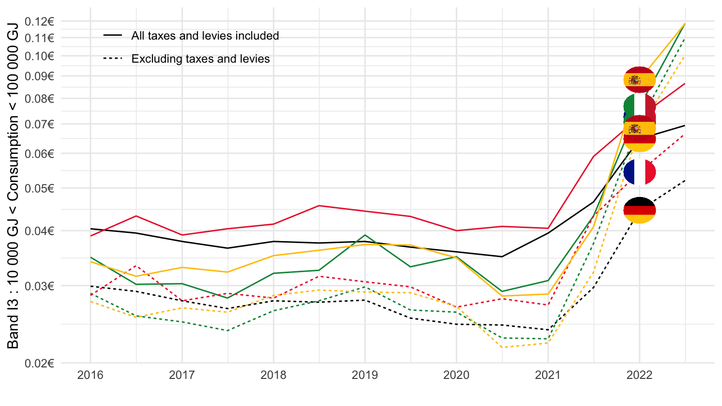

Band D3 : Consumption > 4 000 000 GJ

France, Germany, Italy, Spain

All

nrg_pc_203 %>%
  filter(geo %in% c("FR", "DE", "IT", "ES"),
         tax %in% c("I_TAX", "X_TAX"),
         unit == "KWH",
         consom == "4142906",
         currency == "EUR") %>%
  left_join(geo, by = "geo") %>%
  left_join(tax, by = "tax") %>%
  semester_to_date %>%
  left_join(colors, by = c("Geo" = "country")) %>%
  ggplot + geom_line(aes(x = date, y = values, color = color, linetype = Tax)) +
  scale_color_identity() + theme_minimal()  + add_8flags +
  scale_x_date(breaks = as.Date(paste0(seq(1960, 2025, 2), "-01-01")),
               labels = date_format("%Y")) +
  theme(legend.position = c(0.2, 0.9),
        legend.title = element_blank()) +
  xlab("") + ylab("Consumption > 4 000 000 GJ") +
  scale_y_log10(breaks = seq(0.02, 0.12, 0.01),
                labels = dollar_format(a = .01, pre = "", su = "€"))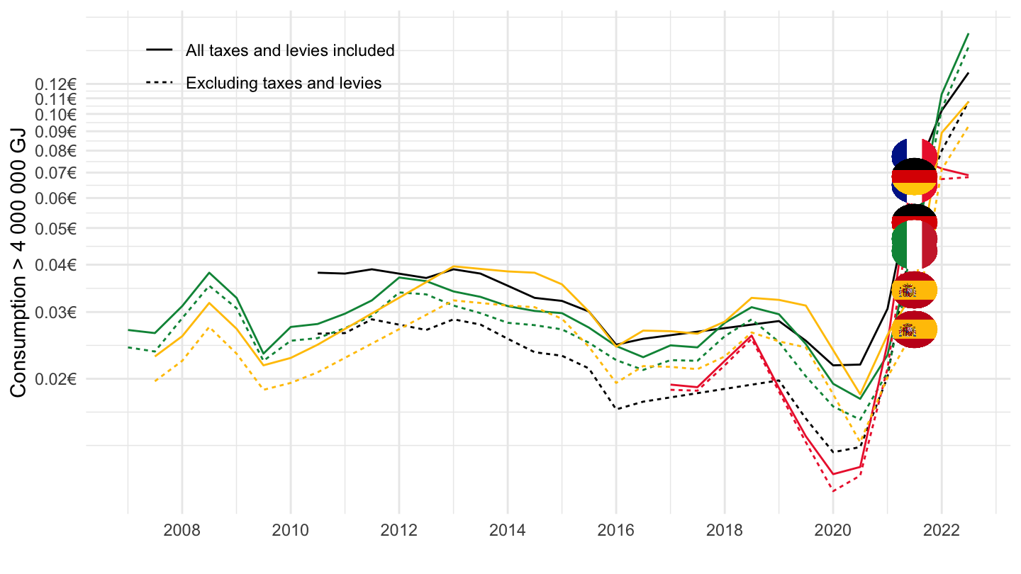

2016-

nrg_pc_203 %>%
  filter(geo %in% c("FR", "DE", "IT", "ES"),
         tax %in% c("I_TAX", "X_TAX"),
         unit == "KWH",
         consom == "4142906",
         currency == "EUR") %>%
  left_join(geo, by = "geo") %>%
  left_join(tax, by = "tax") %>%
  semester_to_date %>%
  filter(date >= as.Date("2016-01-01")) %>%
  left_join(colors, by = c("Geo" = "country")) %>%
  ggplot + geom_line(aes(x = date, y = values, color = color, linetype = Tax)) +
  scale_color_identity() + theme_minimal()  + add_8flags +
  scale_x_date(breaks = as.Date(paste0(seq(1960, 2025, 1), "-01-01")),
               labels = date_format("%Y")) +
  theme(legend.position = c(0.2, 0.9),
        legend.title = element_blank()) +
  xlab("") + ylab("Consumption > 4 000 000 GJ") +
  scale_y_log10(breaks = seq(0.01, 0.30, 0.01),
                labels = dollar_format(a = .01, pre = "", su = "€"))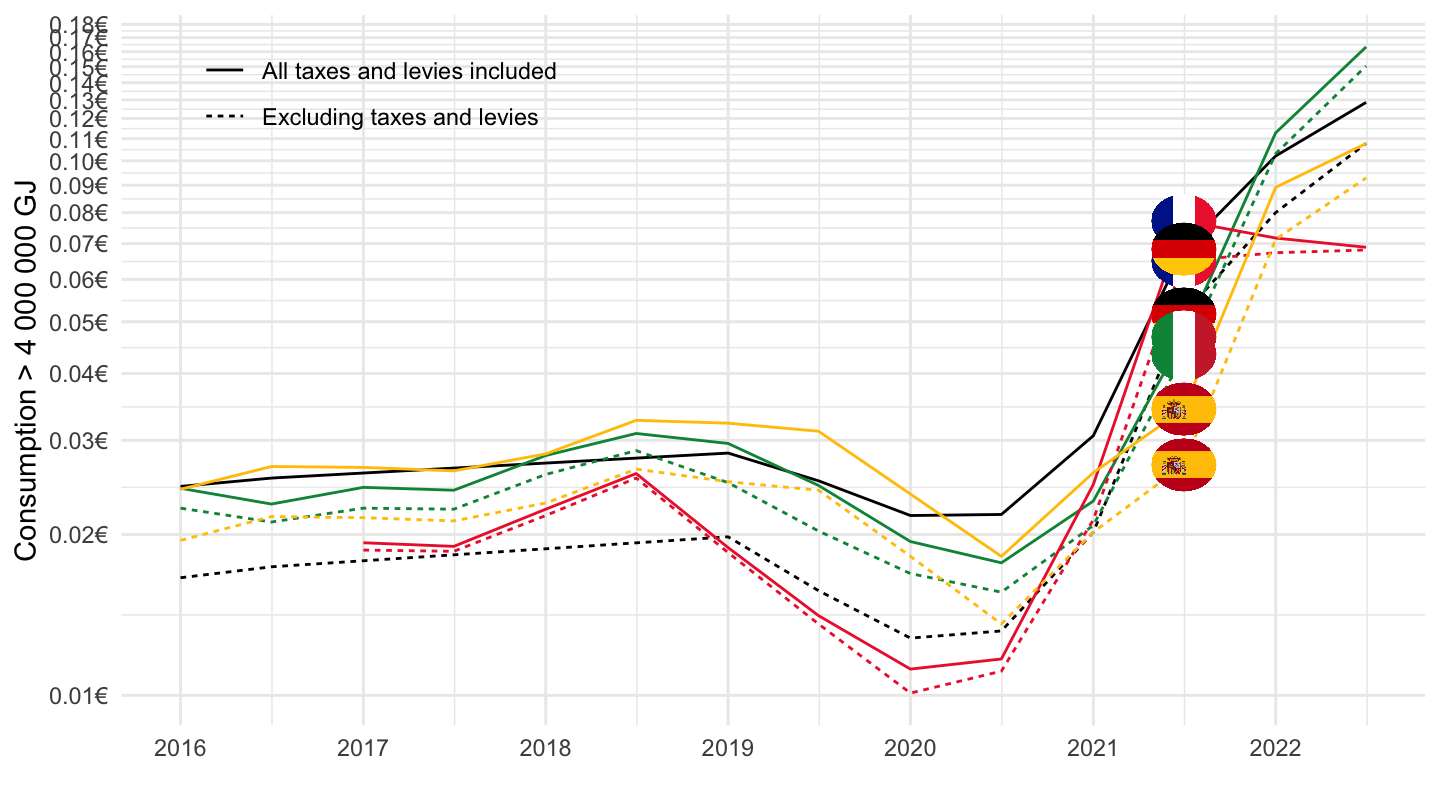

2020-

nrg_pc_203 %>%
  filter(geo %in% c("FR", "DE", "IT", "ES"),
         tax %in% c("I_TAX", "X_TAX"),
         unit == "KWH",
         consom == "4142906",
         currency == "EUR") %>%
  left_join(geo, by = "geo") %>%
  left_join(tax, by = "tax") %>%
  semester_to_date %>%
  filter(date >= as.Date("2020-01-01")) %>%
  left_join(colors, by = c("Geo" = "country")) %>%
  ggplot + geom_line(aes(x = date, y = values, color = color, linetype = Tax)) +
  scale_color_identity() + theme_minimal()  + add_8flags +
  scale_x_date(breaks = as.Date(paste0(seq(1960, 2025, 1), "-01-01")),
               labels = date_format("%Y")) +
  theme(legend.position = c(0.2, 0.9),
        legend.title = element_blank()) +
  xlab("") + ylab("Consumption > 4 000 000 GJ") +
  scale_y_log10(breaks = seq(0.02, 0.12, 0.01),
                labels = dollar_format(a = .01, pre = "", su = "€"))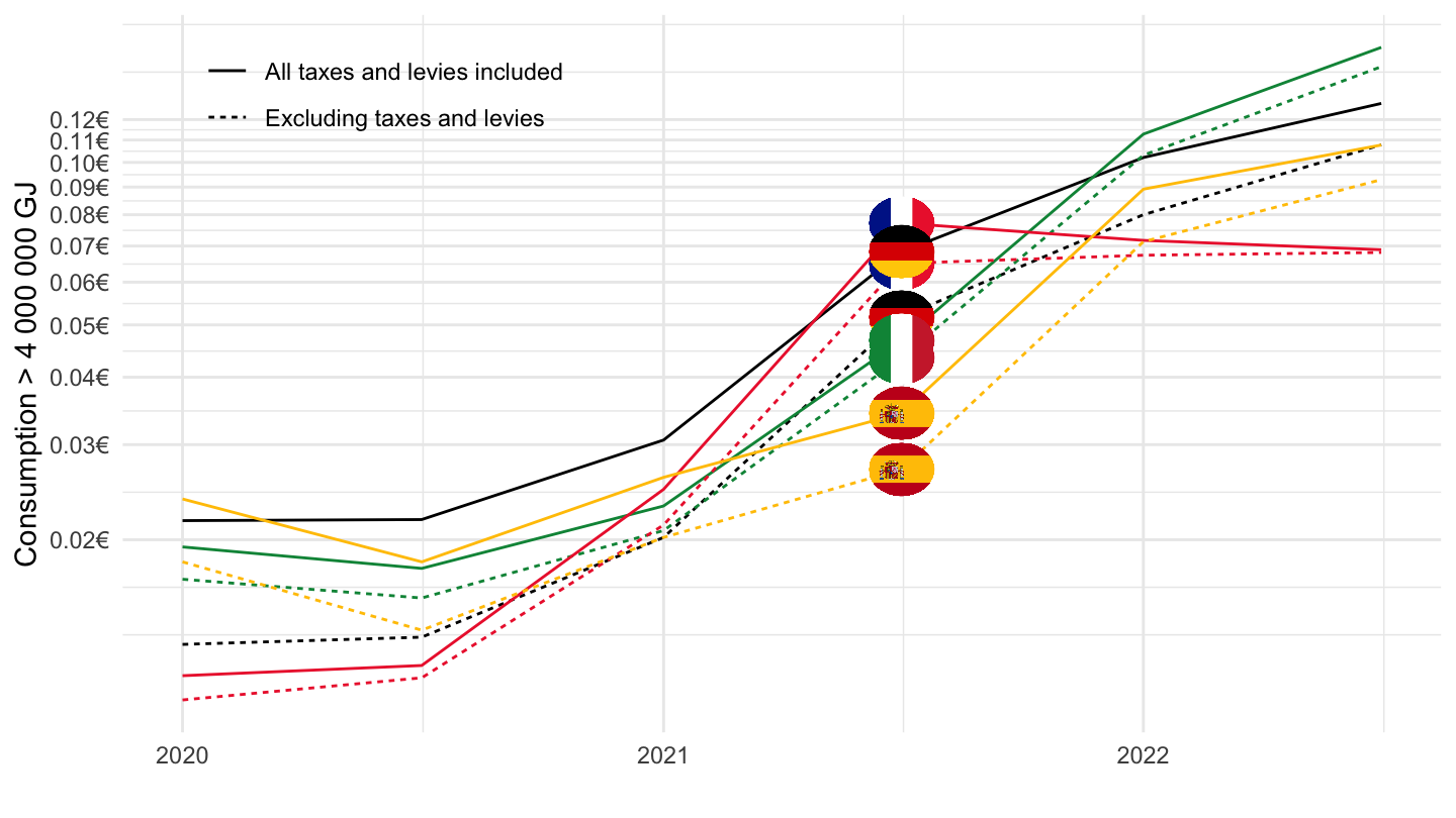

France, Germany, Europe, Spain

Bar

nrg_pc_203 %>%
  filter(geo %in% c("FR", "DE", "EA", "ES"),
         consom == "4142906",
         currency == "EUR",
         unit == "KWH",
         time %in% c("2021S2", "2022S1", "2022S2")) %>%
  select_if(~n_distinct(.) > 1) %>%
  left_join(geo, by = "geo") %>%
  mutate(Geo = ifelse(geo == "EA", "Europe", Geo)) %>%
  spread(tax, values) %>%
  transmute(time, Geo,
            ` Taxes except VAT` = X_VAT-X_TAX,
            `  VAT` = I_TAX-X_VAT,
            `Excluding taxes` = X_TAX) %>%
  gather(Tax, values, - time, -Geo) %>%
  ggplot(., aes(x = time, y = values, fill = Tax)) + 
  geom_bar(stat = "identity",
           position = "stack") +
  facet_grid(~ Geo) + theme_minimal() +
theme(legend.position = "none",
      legend.title = element_blank()) +
  scale_fill_manual(values = viridis(3)[1:3]) +
  scale_y_continuous(breaks = seq(-30, 30, .05),
                labels = dollar_format(a = .01, pre = "", su = "€/kWh"))  +
  xlab("") + ylab("") +
  ggtitle("Natural gas price, HIGH Consumption")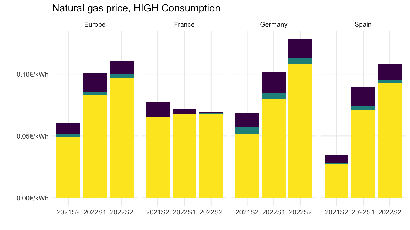

All

nrg_pc_203 %>%
  filter(geo %in% c("FR", "DE", "EA", "ES"),
         tax %in% c("I_TAX", "X_TAX"),
         unit == "KWH",
         consom == "4142906",
         currency == "EUR") %>%
  left_join(geo, by = "geo") %>%
  left_join(tax, by = "tax") %>%
  semester_to_date %>%
  mutate(Geo = ifelse(geo == "EA", "Europe", Geo)) %>%
  left_join(colors, by = c("Geo" = "country")) %>%
  ggplot + geom_line(aes(x = date, y = values, color = color, linetype = Tax)) +
  scale_color_identity() + theme_minimal()  + add_8flags +
  scale_x_date(breaks = as.Date(paste0(seq(1960, 2025, 2), "-01-01")),
               labels = date_format("%Y")) +
  theme(legend.position = c(0.2, 0.9),
        legend.title = element_blank()) +
  xlab("") + ylab("Consumption > 4 000 000 GJ") +
  scale_y_log10(breaks = seq(0.02, 0.2, 0.01),
                labels = dollar_format(a = .01, pre = "", su = "€"))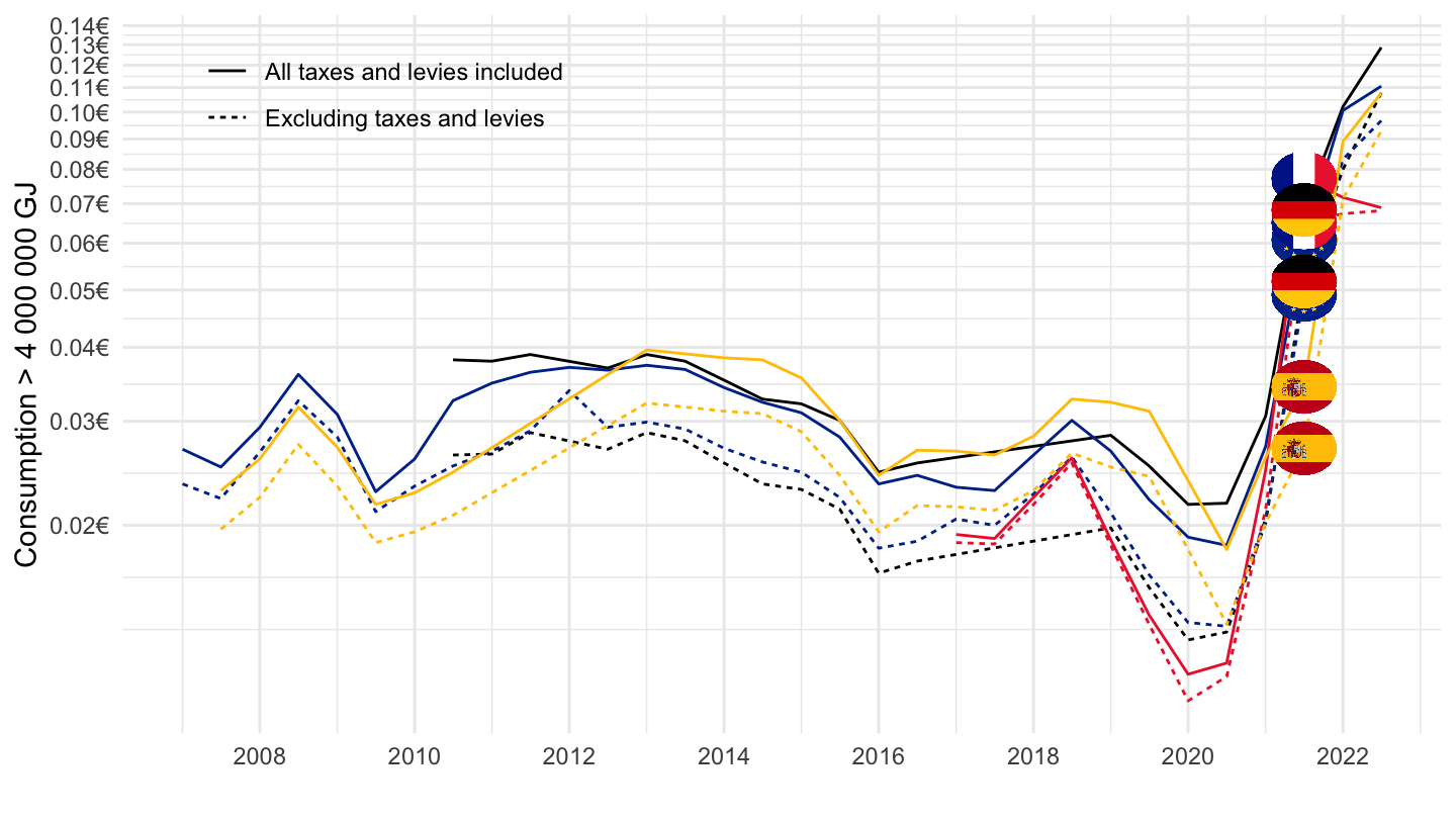

2016-

nrg_pc_203 %>%
  filter(geo %in% c("FR", "DE", "EA", "ES"),
         tax %in% c("I_TAX", "X_TAX"),
         unit == "KWH",
         consom == "4142906",
         currency == "EUR") %>%
  left_join(geo, by = "geo") %>%
  left_join(tax, by = "tax") %>%
  semester_to_date %>%
  filter(date >= as.Date("2016-01-01")) %>%
  mutate(Geo = ifelse(geo == "EA", "Europe", Geo)) %>%
  left_join(colors, by = c("Geo" = "country")) %>%
  ggplot + geom_line(aes(x = date, y = values, color = color, linetype = Tax)) +
  scale_color_identity() + theme_minimal()  + add_8flags +
  scale_x_date(breaks = as.Date(paste0(seq(1960, 2025, 1), "-01-01")),
               labels = date_format("%Y")) +
  theme(legend.position = c(0.2, 0.9),
        legend.title = element_blank()) +
  xlab("") + ylab("Consumption > 4 000 000 GJ") +
  scale_y_log10(breaks = seq(0.02, 0.2, 0.01),
                labels = dollar_format(a = .01, pre = "", su = "€"))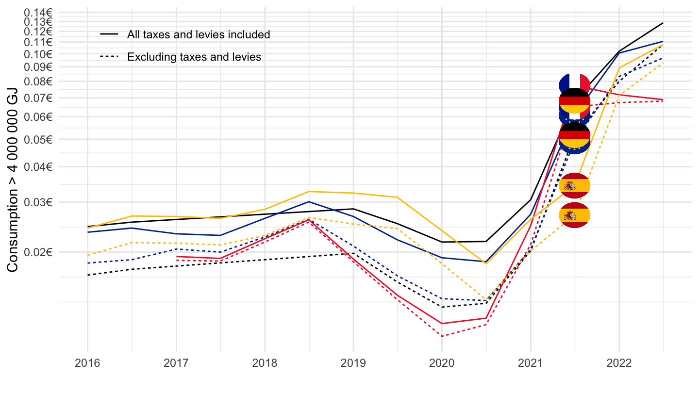

2020-

nrg_pc_203 %>%
  filter(geo %in% c("FR", "DE", "EA", "ES"),
         tax %in% c("I_TAX", "X_TAX"),
         unit == "KWH",
         consom == "4142906",
         currency == "EUR") %>%
  left_join(geo, by = "geo") %>%
  left_join(tax, by = "tax") %>%
  semester_to_date %>%
  filter(date >= as.Date("2020-01-01")) %>%
  mutate(Geo = ifelse(geo == "EA", "Europe", Geo)) %>%
  left_join(colors, by = c("Geo" = "country")) %>%
  ggplot + geom_line(aes(x = date, y = values, color = color, linetype = Tax)) +
  scale_color_identity() + theme_minimal()  + add_8flags +
  scale_x_date(breaks = as.Date(paste0(seq(1960, 2025, 1), "-01-01")),
               labels = date_format("%Y")) +
  theme(legend.position = c(0.2, 0.9),
        legend.title = element_blank()) +
  xlab("") + ylab("Consumption > 4 000 000 GJ") +
  scale_y_log10(breaks = seq(0.02, 0.2, 0.01),
                labels = dollar_format(a = .01, pre = "", su = "€"))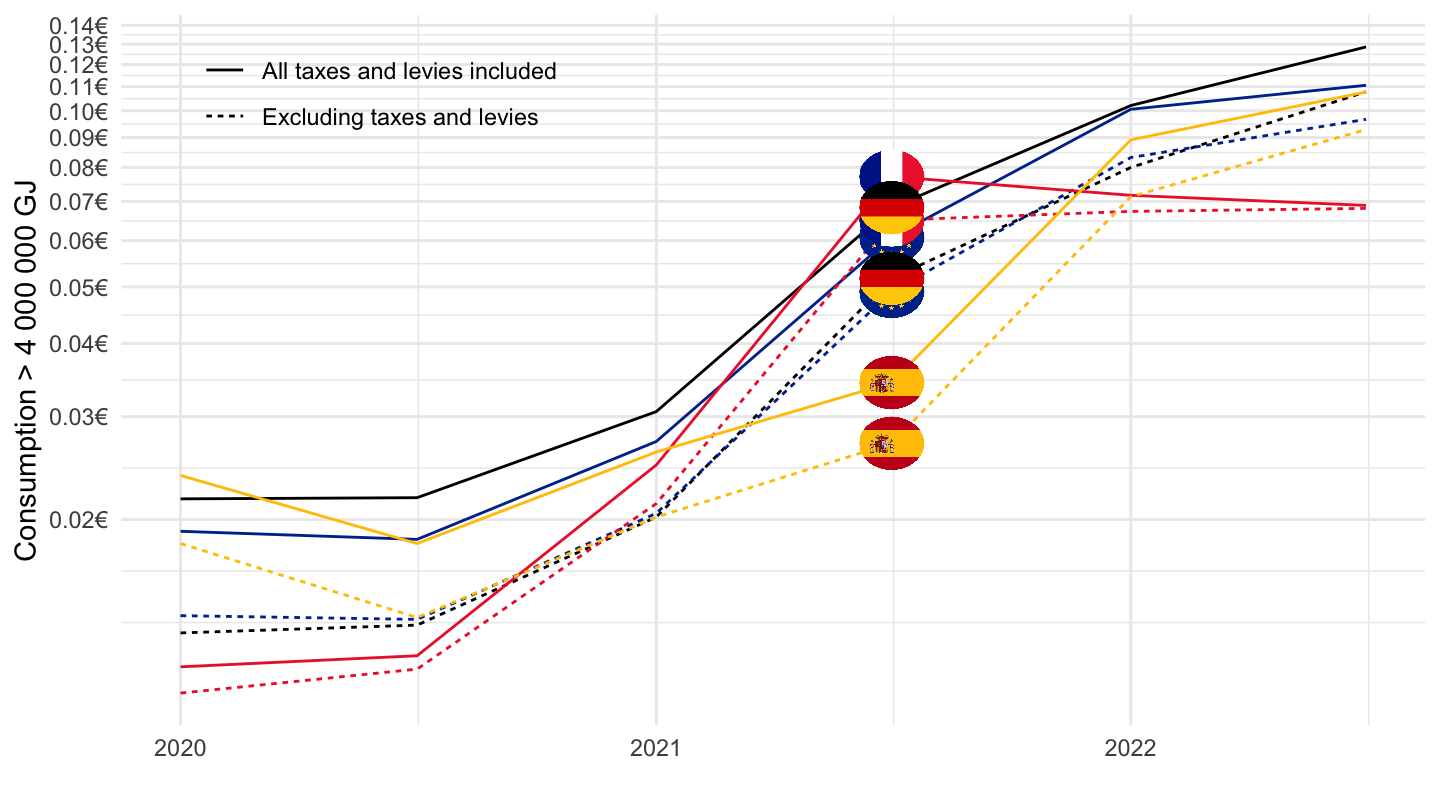

Example

France

Log

nrg_pc_203 %>%
  filter(geo == "FR",
         unit == "KWH",
         currency == "EUR") %>%
  left_join(tax, by = "tax") %>%
  left_join(consom, by = "consom") %>%
  select_if(~ n_distinct(.) > 1) %>%
  semester_to_date %>%
  ggplot + geom_line(aes(x = date, y = values, color = Consom, linetype = Tax)) +
  theme_minimal() + xlab("") + ylab("") +
  scale_x_date(breaks = seq(1920, 2025, 2) %>% paste0("-01-01") %>% as.Date,
               labels = date_format("%Y")) +
  scale_y_log10(breaks = seq(0, 1, 0.01)) +
  theme(legend.position = c(0.45, 0.7),
        legend.title = element_blank())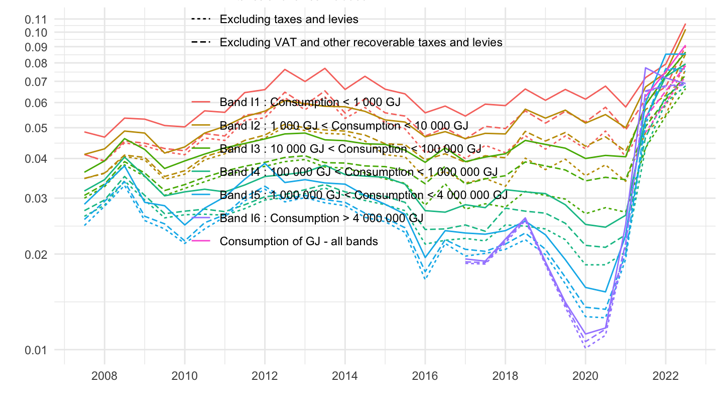

Linear

nrg_pc_203 %>%
  filter(geo == "FR",
         unit == "KWH",
         currency == "EUR") %>%
  left_join(tax, by = "tax") %>%
  left_join(consom, by = "consom") %>%
  select_if(~ n_distinct(.) > 1) %>%
  semester_to_date %>%
  ggplot + geom_line(aes(x = date, y = values, color = Consom, linetype = Tax)) +
  theme_minimal() + xlab("") + ylab("") +
  scale_x_date(breaks = seq(1920, 2025, 2) %>% paste0("-01-01") %>% as.Date,
               labels = date_format("%Y")) +
  scale_y_continuous(breaks = seq(0, 1, 0.01)) +
  theme(legend.position = c(0.45, 0.7),
        legend.title = element_blank())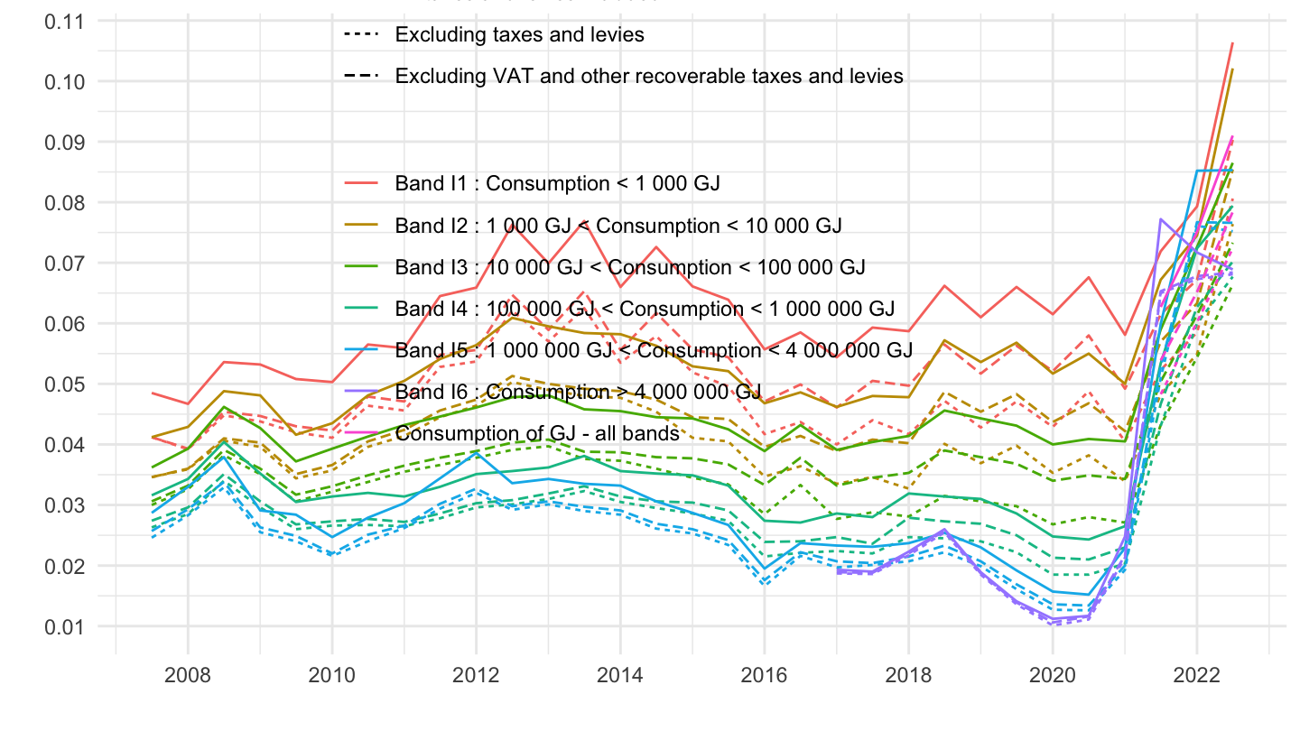

Germany

Log

nrg_pc_203 %>%
  filter(geo == "DE",
         unit == "KWH",
         currency == "EUR") %>%
  left_join(tax, by = "tax") %>%
  left_join(consom, by = "consom") %>%
  select_if(~ n_distinct(.) > 1) %>%
  semester_to_date %>%
  ggplot + geom_line(aes(x = date, y = values, color = Consom, linetype = Tax)) +
  theme_minimal() + xlab("") + ylab("") +
  scale_x_date(breaks = seq(1920, 2025, 2) %>% paste0("-01-01") %>% as.Date,
               labels = date_format("%Y")) +
  scale_y_log10(breaks = seq(0, 1, 0.01)) +
  theme(legend.position = c(0.45, 0.7),
        legend.title = element_blank())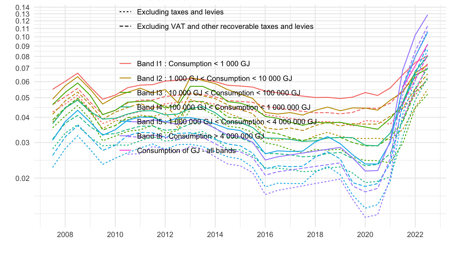

Linear

nrg_pc_203 %>%
  filter(geo == "DE",
         unit == "KWH",
         currency == "EUR") %>%
  left_join(tax, by = "tax") %>%
  left_join(consom, by = "consom") %>%
  select_if(~ n_distinct(.) > 1) %>%
  semester_to_date %>%
  ggplot + geom_line(aes(x = date, y = values, color = Consom, linetype = Tax)) +
  theme_minimal() + xlab("") + ylab("") +
  scale_x_date(breaks = seq(1920, 2025, 2) %>% paste0("-01-01") %>% as.Date,
               labels = date_format("%Y")) +
  scale_y_continuous(breaks = seq(0, 1, 0.01)) +
  theme(legend.position = c(0.45, 0.7),
        legend.title = element_blank())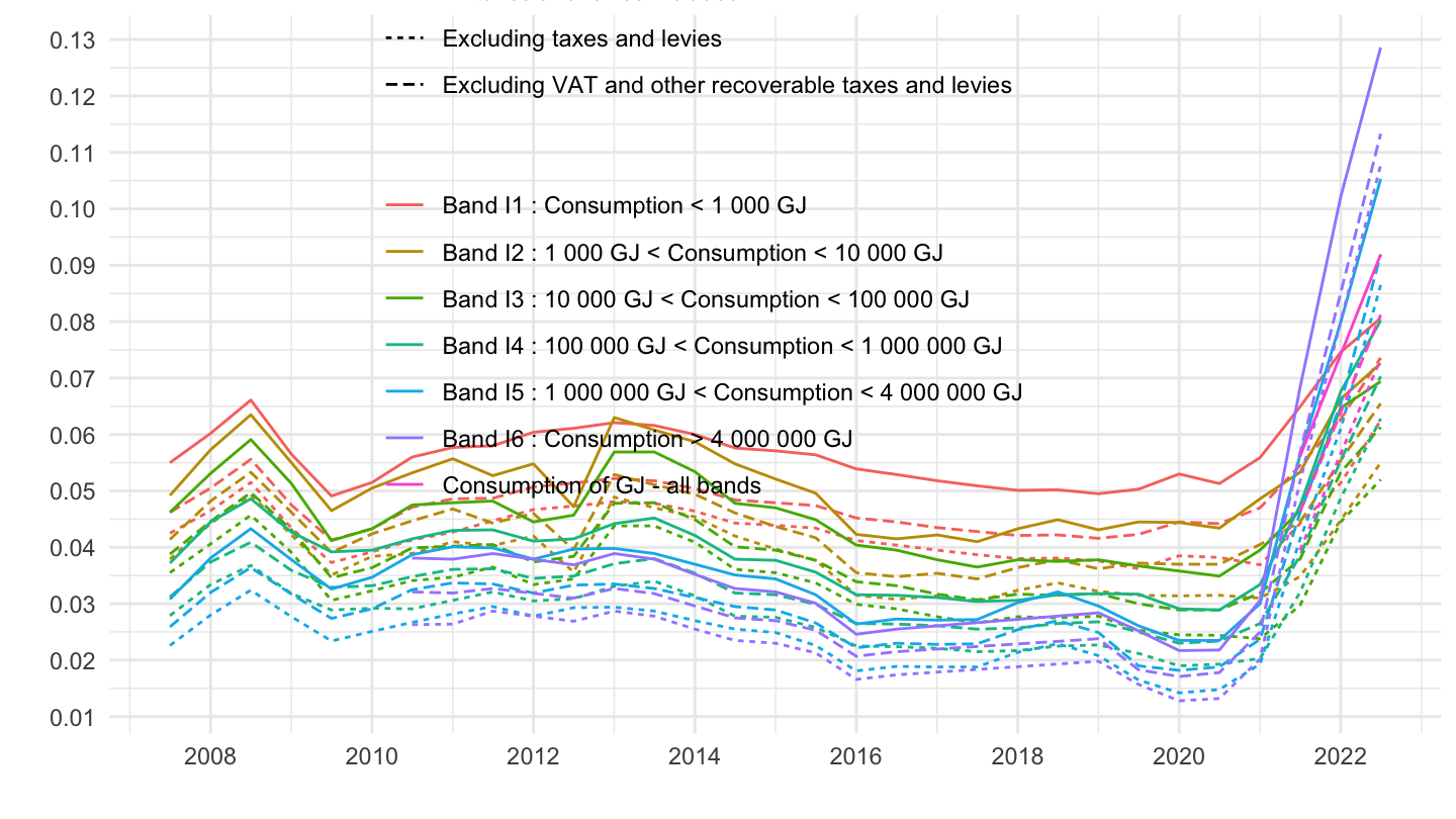

Italy

Log

nrg_pc_203 %>%
  filter(geo == "IT",
         unit == "KWH",
         currency == "EUR") %>%
  left_join(tax, by = "tax") %>%
  left_join(consom, by = "consom") %>%
  select_if(~ n_distinct(.) > 1) %>%
  semester_to_date %>%
  ggplot + geom_line(aes(x = date, y = values, color = Consom, linetype = Tax)) +
  theme_minimal() + xlab("") + ylab("") +
  scale_x_date(breaks = seq(1920, 2025, 2) %>% paste0("-01-01") %>% as.Date,
               labels = date_format("%Y")) +
  scale_y_log10(breaks = seq(0, 1, 0.01)) +
  theme(legend.position = c(0.45, 0.7),
        legend.title = element_blank())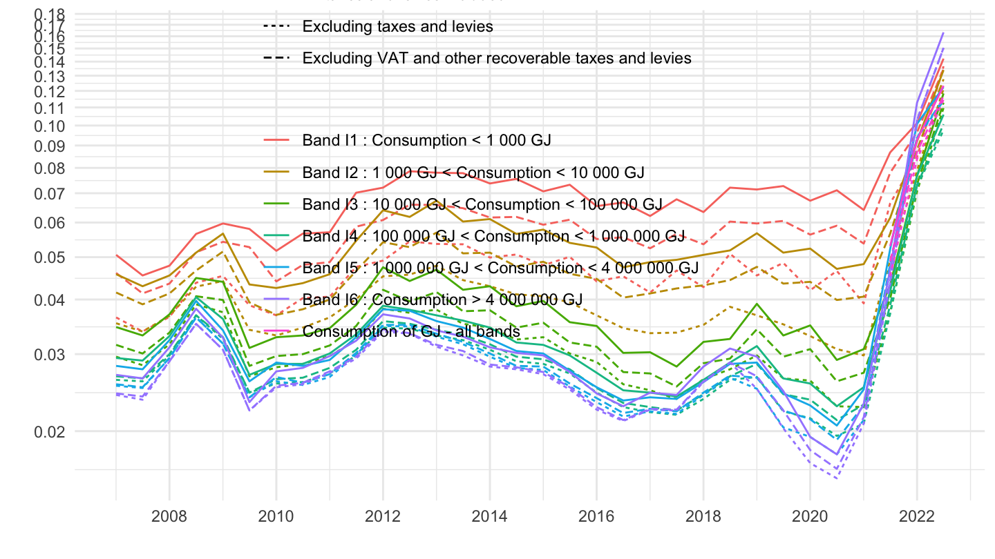

Linear

nrg_pc_203 %>%
  filter(geo == "IT",
         unit == "KWH",
         currency == "EUR") %>%
  left_join(tax, by = "tax") %>%
  left_join(consom, by = "consom") %>%
  select_if(~ n_distinct(.) > 1) %>%
  semester_to_date %>%
  ggplot + geom_line(aes(x = date, y = values, color = Consom, linetype = Tax)) +
  theme_minimal() + xlab("") + ylab("") +
  scale_x_date(breaks = seq(1920, 2025, 2) %>% paste0("-01-01") %>% as.Date,
               labels = date_format("%Y")) +
  scale_y_continuous(breaks = seq(0, 1, 0.01)) +
  theme(legend.position = c(0.45, 0.7),
        legend.title = element_blank())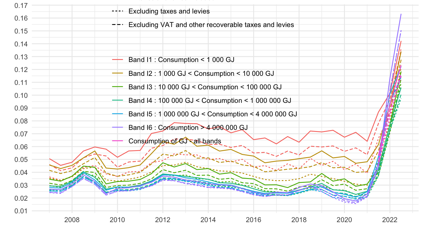

Spain

nrg_pc_203 %>%
  filter(geo == "ES",
         unit == "KWH",
         currency == "EUR") %>%
  left_join(tax, by = "tax") %>%
  left_join(consom, by = "consom") %>%
  select_if(~ n_distinct(.) > 1) %>%
  semester_to_date %>%
  ggplot + geom_line(aes(x = date, y = values, color = Consom, linetype = Tax)) +
  theme_minimal() + xlab("") + ylab("") +
  scale_x_date(breaks = seq(1920, 2025, 2) %>% paste0("-01-01") %>% as.Date,
               labels = date_format("%Y")) +
  scale_y_log10(breaks = seq(0, 1, 0.01)) +
  theme(legend.position = c(0.45, 0.7),
        legend.title = element_blank())