Consumer price indices (CPIs)
Data - OECD
Info
Last observation: Monthly: 2026-03 (N = 209) · Quarterly: 2026-Q1 (N = 162) · Annual: 2025 (N = 4,867)
First observation: Monthly: NA (N = 10) · Quarterly: NA (N = 15) · Annual: NA (N = 36)
Last data update: 16 Apr 2026, 03:33. Last compile: 16 Apr 2026, 15:43
Structure
Europe vs. US
1996-
Code
PRICES_ALL %>%

  filter(EXPENDITURE == "_T",
         REF_AREA %in% c("EA20", "USA"),
         ADJUSTMENT == "N",
         MEASURE == "CPI",
         TRANSFORMATION == "_Z",
         FREQ == "M") %>%
  month_to_date() %>%
  filter(date >= as.Date("1996-01-01")) %>%
  group_by(Ref_area, Methodology) %>%
  arrange(date) %>%
  mutate(obsValue = 100*obsValue/obsValue[1]) %>%
  mutate(Ref_area = ifelse(REF_AREA == "EA20", "Europe", Ref_area)) %>%
  left_join(colors, by = c("Ref_area"  = "country")) %>%
  ggplot(.) + geom_line(aes(x = date, y = obsValue, color = color, linetype = Methodology)) +
  scale_color_identity() +
  scale_linetype_manual(values = c("dashed", "solid")) + add_flags +
  theme_minimal() + xlab("") + ylab("Price Index") +
  scale_x_date(breaks = seq(1960, 2100, 1) %>% paste0("-01-01") %>% as.Date,
               labels = date_format("%Y")) +
  theme(legend.position = c(0.35, 0.8),
        legend.title = element_blank(),
        axis.text.x = element_text(angle = 45, vjust = 1, hjust = 1)) +
  scale_y_log10(breaks = seq(10, 200, 5))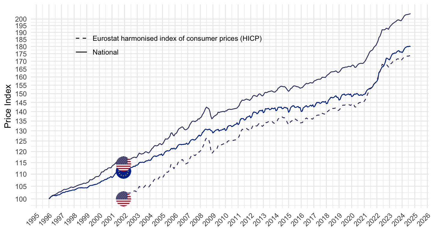
1996-
Code
PRICES_ALL %>%

  filter(EXPENDITURE == "_T",
         REF_AREA %in% c("EA20", "USA"),
         ADJUSTMENT == "N",
         MEASURE == "CPI",
         TRANSFORMATION == "_Z",
         FREQ == "M") %>%
  month_to_date() %>%
  filter(date >= as.Date("2002-01-01")) %>%
  group_by(Ref_area, Methodology) %>%
  arrange(date) %>%
  mutate(obsValue = 100*obsValue/obsValue[1]) %>%
  mutate(Ref_area = ifelse(REF_AREA == "EA20", "Europe", Ref_area)) %>%
  left_join(colors, by = c("Ref_area"  = "country")) %>%
  ggplot(.) + geom_line(aes(x = date, y = obsValue, color = color, linetype = Methodology)) +
  scale_color_identity() +
  scale_linetype_manual(values = c("dashed", "solid")) + add_flags +
  theme_minimal() + xlab("") + ylab("Price Index") +
  scale_x_date(breaks = seq(1960, 2100, 1) %>% paste0("-01-01") %>% as.Date,
               labels = date_format("%Y")) +
  theme(legend.position = c(0.35, 0.8),
        legend.title = element_blank(),
        axis.text.x = element_text(angle = 45, vjust = 1, hjust = 1)) +
  scale_y_log10(breaks = seq(10, 200, 5))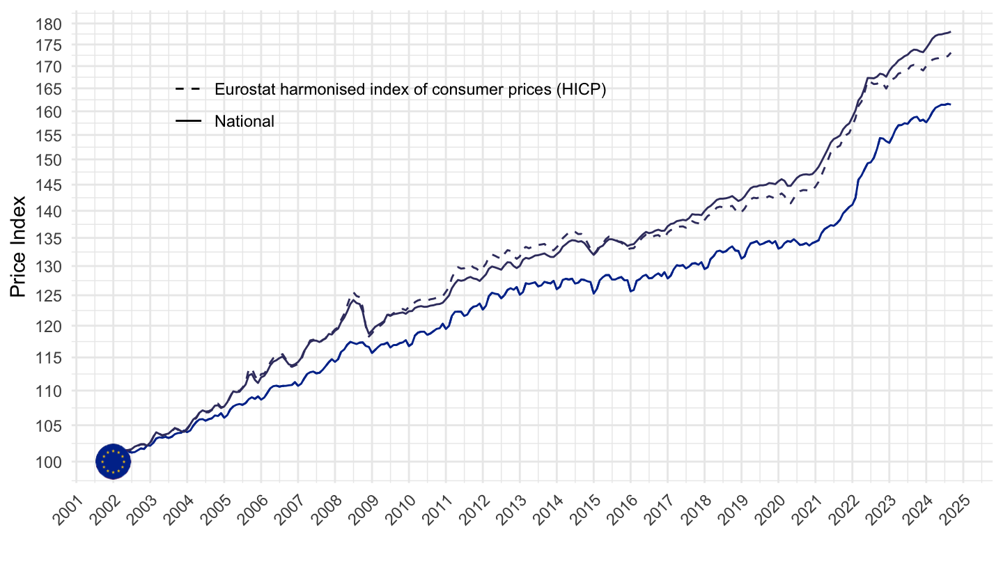
2017-
Code
PRICES_ALL %>%
  filter(EXPENDITURE == "_T",
         REF_AREA %in% c("EA20", "USA"),
         ADJUSTMENT == "N",
         MEASURE == "CPI",
         TRANSFORMATION == "_Z",
         FREQ == "M") %>%


  month_to_date() %>%
  filter(date >= as.Date("2017-01-01")) %>%
  group_by(Ref_area, Methodology) %>%
  arrange(date) %>%
  mutate(obsValue = 100*obsValue/obsValue[1]) %>%
  mutate(Ref_area = ifelse(REF_AREA == "EA20", "Europe", Ref_area)) %>%
  left_join(colors, by = c("Ref_area"  = "country")) %>%
  ggplot(.) + geom_line(aes(x = date, y = obsValue, color = color, linetype = Methodology)) +
  scale_color_identity() +
  scale_linetype_manual(values = c("dashed", "solid")) + add_3flags +
  theme_minimal() + xlab("") + ylab("Price Index") +
  scale_x_date(breaks = seq(1960, 2100, 1) %>% paste0("-01-01") %>% as.Date,
               labels = date_format("%Y")) +
  theme(legend.position = c(0.35, 0.8),
        legend.title = element_blank(),
        axis.text.x = element_text(angle = 45, vjust = 1, hjust = 1)) +
  scale_y_log10(breaks = seq(10, 200, 5))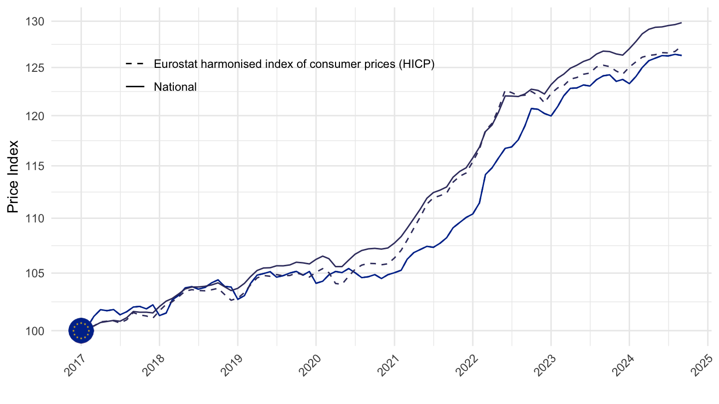
France vs. Germany vs. Italy
1996-
Code
PRICES_ALL %>%

  filter(EXPENDITURE == "_T",
         REF_AREA %in% c("FRA", "DEU", "ITA"),
         ADJUSTMENT == "N",
         MEASURE == "CPI",
         TRANSFORMATION == "_Z",
         FREQ == "M") %>%
  month_to_date() %>%
  filter(date >= as.Date("1996-01-01")) %>%
  group_by(Ref_area, Methodology) %>%
  arrange(date) %>%
  mutate(obsValue = 100*obsValue/obsValue[1]) %>%
  left_join(colors, by = c("Ref_area"  = "country")) %>%
  ggplot(.) + geom_line(aes(x = date, y = obsValue, color = color, linetype = Methodology)) +
  scale_color_identity() +
  scale_linetype_manual(values = c("dashed", "solid")) + add_flags +
  theme_minimal() + xlab("") + ylab("Price Index") +
  scale_x_date(breaks = seq(1960, 2100, 1) %>% paste0("-01-01") %>% as.Date,
               labels = date_format("%Y")) +
  theme(legend.position = c(0.35, 0.8),
        legend.title = element_blank(),
        axis.text.x = element_text(angle = 45, vjust = 1, hjust = 1)) +
  scale_y_log10(breaks = seq(10, 200, 5))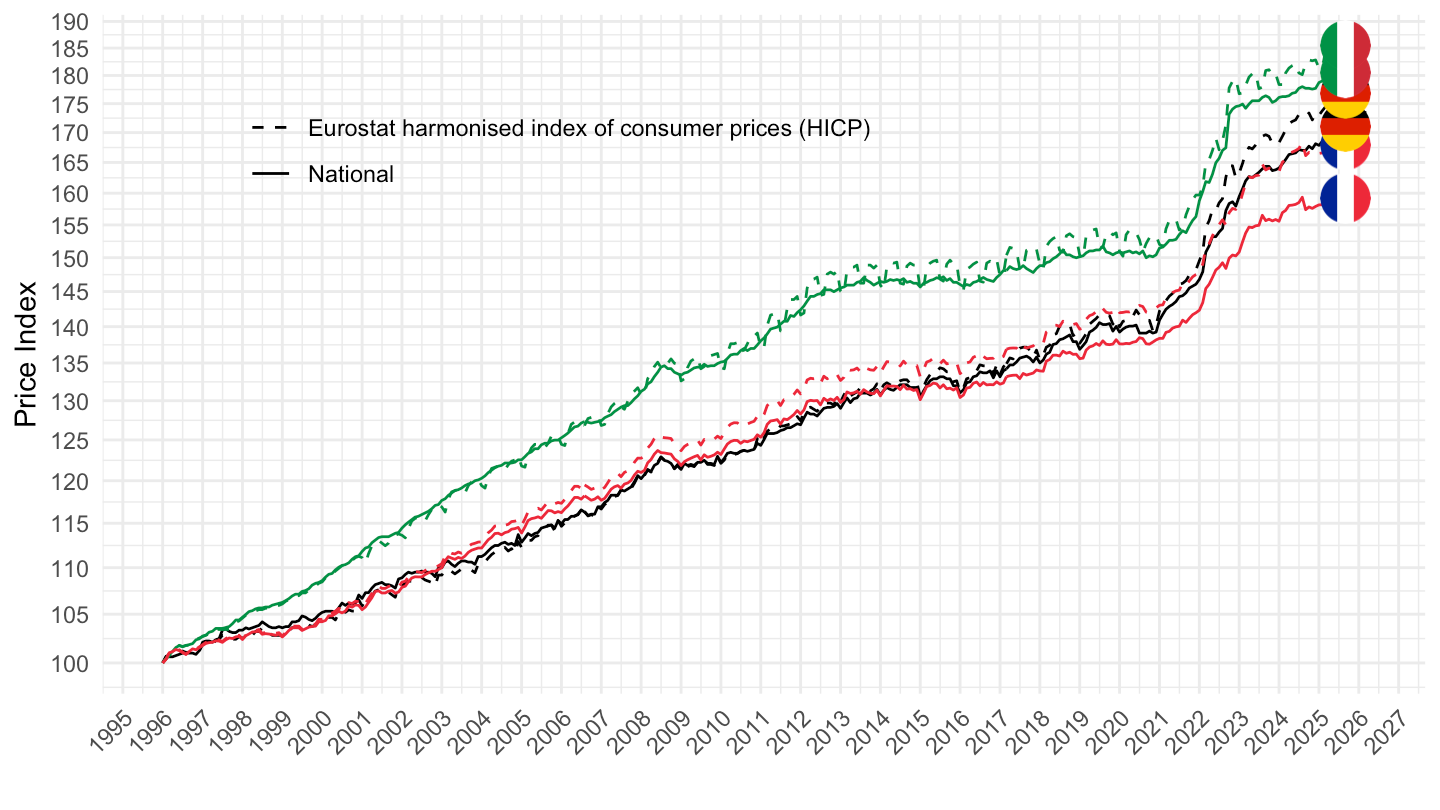
1999-
Code
PRICES_ALL %>%

  filter(EXPENDITURE == "_T",
         REF_AREA %in% c("FRA", "DEU", "ITA"),
         ADJUSTMENT == "N",
         MEASURE == "CPI",
         TRANSFORMATION == "_Z",
         FREQ == "M") %>%
  month_to_date() %>%
  filter(date >= as.Date("1999-01-01")) %>%
  group_by(Ref_area, Methodology) %>%
  arrange(date) %>%
  mutate(obsValue = 100*obsValue/obsValue[1]) %>%
  left_join(colors, by = c("Ref_area"  = "country")) %>%
  ggplot(.) + geom_line(aes(x = date, y = obsValue, color = color, linetype = Methodology)) +
  scale_color_identity() +
  scale_linetype_manual(values = c("dashed", "solid")) + add_flags +
  theme_minimal() + xlab("") + ylab("Price Index") +
  scale_x_date(breaks = seq(1960, 2100, 1) %>% paste0("-01-01") %>% as.Date,
               labels = date_format("%Y")) +
  theme(legend.position = c(0.35, 0.8),
        legend.title = element_blank(),
        axis.text.x = element_text(angle = 45, vjust = 1, hjust = 1)) +
  scale_y_log10(breaks = seq(10, 200, 5))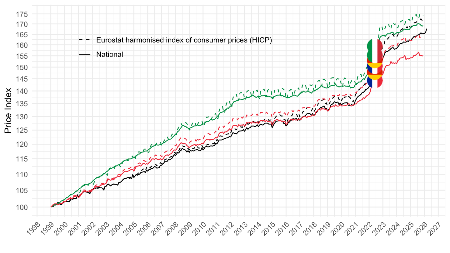
2017-
Code
PRICES_ALL %>%

  filter(EXPENDITURE == "_T",
         REF_AREA %in% c("FRA", "DEU", "ITA"),
         ADJUSTMENT == "N",
         MEASURE == "CPI",
         TRANSFORMATION == "_Z",
         FREQ == "M") %>%
  month_to_date() %>%
  filter(date >= as.Date("2017-01-01")) %>%
  group_by(Ref_area, Methodology) %>%
  arrange(date) %>%
  mutate(obsValue = 100*obsValue/obsValue[1]) %>%
  left_join(colors, by = c("Ref_area"  = "country")) %>%
  ggplot(.) + geom_line(aes(x = date, y = obsValue, color = color, linetype = Methodology)) +
  scale_color_identity() +
  scale_linetype_manual(values = c("dashed", "solid")) + add_flags +
  theme_minimal() + xlab("") + ylab("Price Index") +
  scale_x_date(breaks = seq(1960, 2100, 1) %>% paste0("-01-01") %>% as.Date,
               labels = date_format("%Y")) +
  theme(legend.position = c(0.35, 0.8),
        legend.title = element_blank(),
        axis.text.x = element_text(angle = 45, vjust = 1, hjust = 1)) +
  scale_y_log10(breaks = seq(10, 200, 5))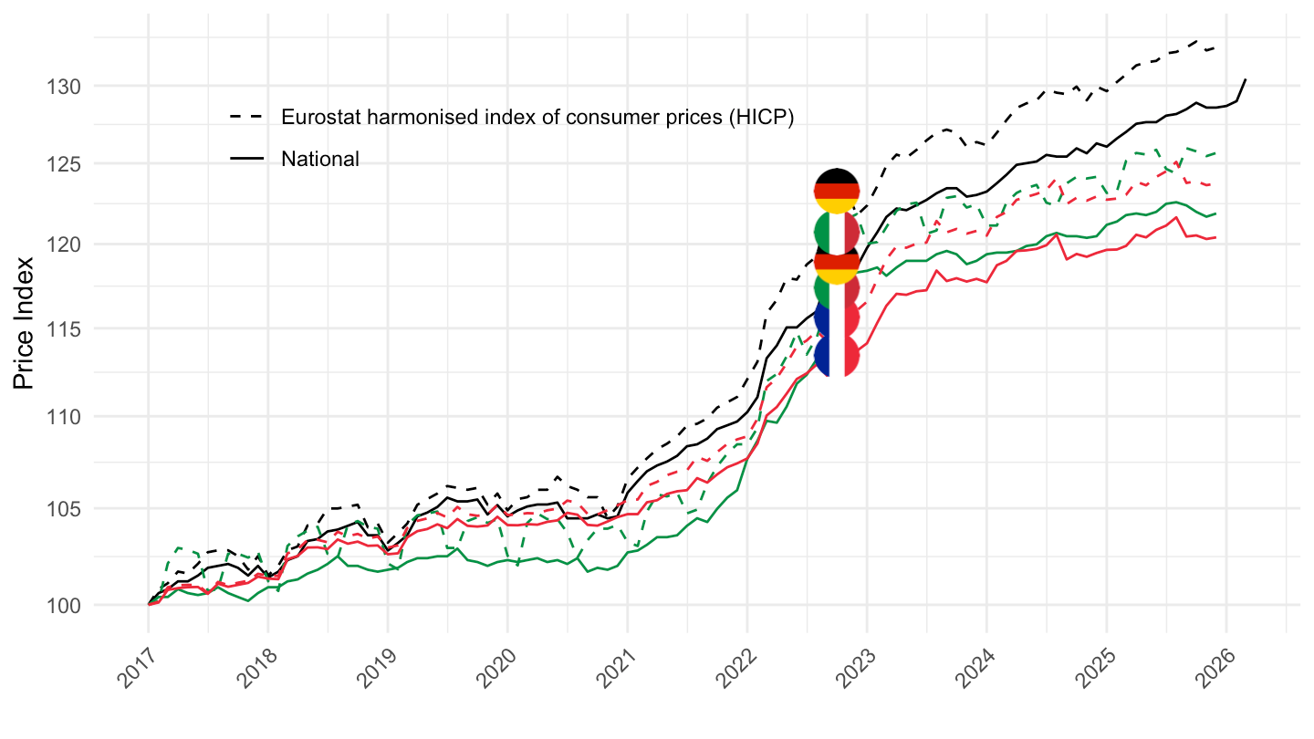
France vs. Germany vs. Italy vs. Netherlands vs. Spain
1996-
Code
PRICES_ALL %>%

  filter(EXPENDITURE == "_T",
         REF_AREA %in% c("FRA", "ESP", "NLD", "DEU", "ITA"),
         ADJUSTMENT == "N",
         MEASURE == "CPI",
         TRANSFORMATION == "_Z",
         FREQ == "M") %>%
  month_to_date() %>%
  filter(date >= as.Date("1996-01-01")) %>%
  group_by(Ref_area, Methodology) %>%
  arrange(date) %>%
  mutate(obsValue = 100*obsValue/obsValue[1]) %>%
  left_join(colors, by = c("Ref_area"  = "country")) %>%
  ggplot(.) + geom_line(aes(x = date, y = obsValue, color = color, linetype = Methodology)) +
  scale_color_identity() +
  scale_linetype_manual(values = c("dashed", "solid")) + add_flags +
  theme_minimal() + xlab("") + ylab("Price Index") +
  scale_x_date(breaks = seq(1960, 2100, 1) %>% paste0("-01-01") %>% as.Date,
               labels = date_format("%Y")) +
  theme(legend.position = c(0.35, 0.8),
        legend.title = element_blank(),
        axis.text.x = element_text(angle = 45, vjust = 1, hjust = 1)) +
  scale_y_log10(breaks = seq(10, 200, 5))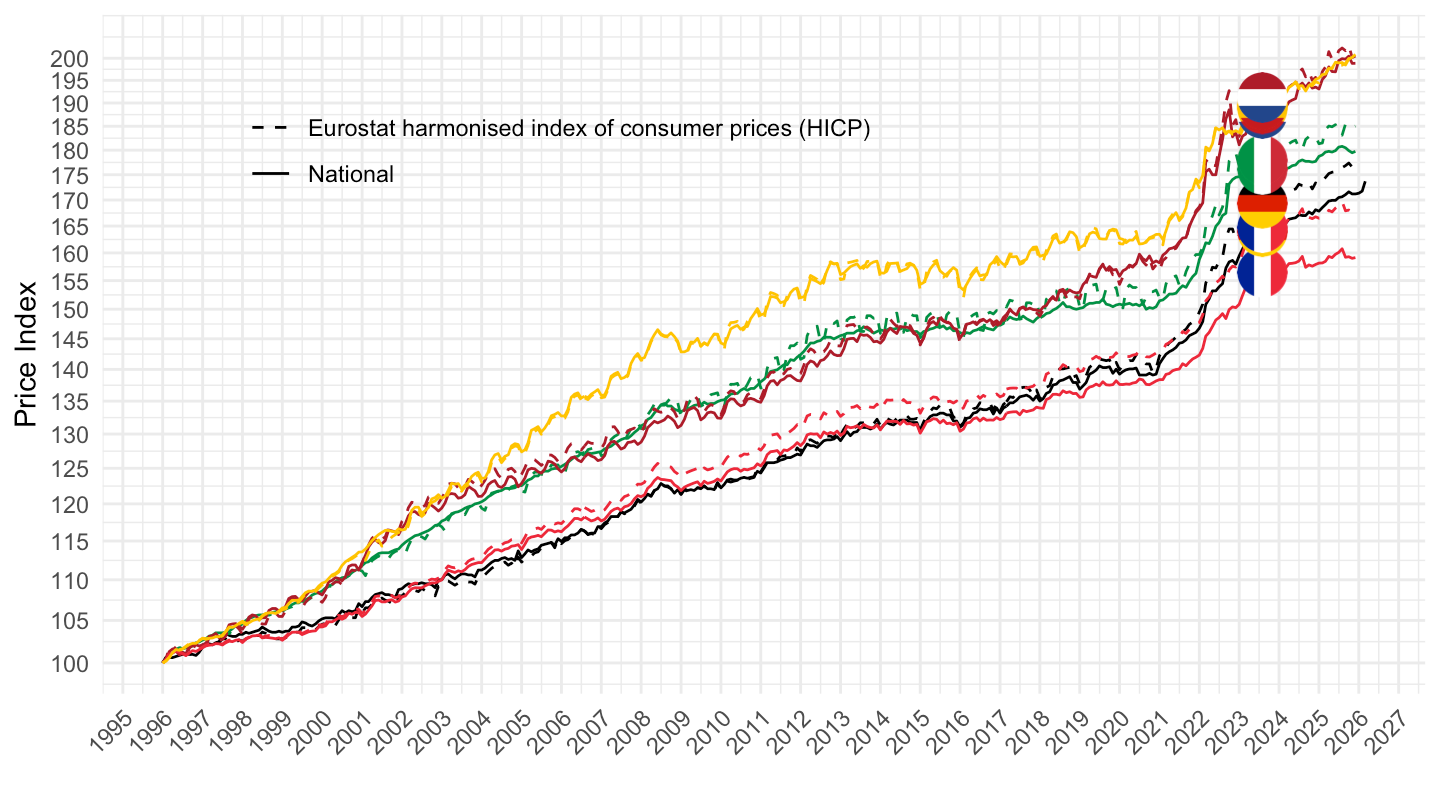
1999-
Code
PRICES_ALL %>%

  filter(EXPENDITURE == "_T",
         REF_AREA %in% c("FRA", "ESP", "NLD", "DEU", "ITA"),
         ADJUSTMENT == "N",
         MEASURE == "CPI",
         TRANSFORMATION == "_Z",
         FREQ == "M") %>%
  month_to_date() %>%
  filter(date >= as.Date("1999-01-01")) %>%
  group_by(Ref_area, Methodology) %>%
  arrange(date) %>%
  mutate(obsValue = 100*obsValue/obsValue[1]) %>%
  left_join(colors, by = c("Ref_area"  = "country")) %>%
  ggplot(.) + geom_line(aes(x = date, y = obsValue, color = color, linetype = Methodology)) +
  scale_color_identity() +
  scale_linetype_manual(values = c("dashed", "solid")) + add_flags +
  theme_minimal() + xlab("") + ylab("Price Index") +
  scale_x_date(breaks = seq(1960, 2100, 1) %>% paste0("-01-01") %>% as.Date,
               labels = date_format("%Y")) +
  theme(legend.position = c(0.35, 0.8),
        legend.title = element_blank(),
        axis.text.x = element_text(angle = 45, vjust = 1, hjust = 1)) +
  scale_y_log10(breaks = seq(10, 200, 5))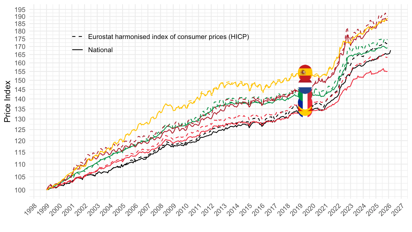
2017-
Code
PRICES_ALL %>%

  filter(EXPENDITURE == "_T",
         REF_AREA %in% c("FRA", "ESP", "NLD", "DEU", "ITA"),
         ADJUSTMENT == "N",
         MEASURE == "CPI",
         TRANSFORMATION == "_Z",
         FREQ == "M") %>%
  month_to_date() %>%
  filter(date >= as.Date("2017-01-01")) %>%
  group_by(Ref_area, Methodology) %>%
  arrange(date) %>%
  mutate(obsValue = 100*obsValue/obsValue[1]) %>%
  left_join(colors, by = c("Ref_area"  = "country")) %>%
  ggplot(.) + geom_line(aes(x = date, y = obsValue, color = color, linetype = Methodology)) +
  scale_color_identity() +
  scale_linetype_manual(values = c("dashed", "solid")) + add_flags +
  theme_minimal() + xlab("") + ylab("Price Index") +
  scale_x_date(breaks = seq(1960, 2100, 1) %>% paste0("-01-01") %>% as.Date,
               labels = date_format("%Y")) +
  theme(legend.position = c(0.35, 0.8),
        legend.title = element_blank(),
        axis.text.x = element_text(angle = 45, vjust = 1, hjust = 1)) +
  scale_y_log10(breaks = seq(10, 200, 5))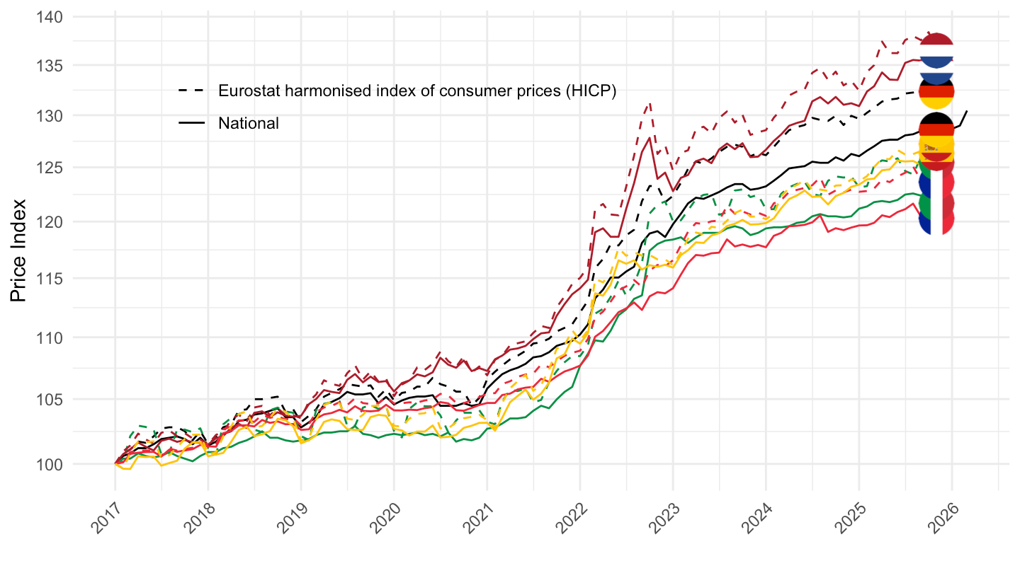
France vs. Germany vs. Italy vs. Netherlands vs. Spain
2017-
Code
PRICES_ALL %>%

  filter(EXPENDITURE == "_T",
         REF_AREA %in% c("FRA", "ESP", "NLD", "DEU"),
         ADJUSTMENT == "N",
         MEASURE == "CPI",
         TRANSFORMATION == "_Z",
         FREQ == "M") %>%
  month_to_date() %>%
  filter(date >= as.Date("2017-01-01")) %>%
  group_by(Ref_area, Methodology) %>%
  arrange(date) %>%
  mutate(obsValue = 100*obsValue/obsValue[1]) %>%
  left_join(colors, by = c("Ref_area"  = "country")) %>%
  ggplot(.) + geom_line(aes(x = date, y = obsValue, color = color, linetype = Methodology)) +
  scale_color_identity() +
  scale_linetype_manual(values = c("dashed", "solid")) + add_flags +
  theme_minimal() + xlab("") + ylab("Price Index") +
  scale_x_date(breaks = seq(1960, 2100, 1) %>% paste0("-01-01") %>% as.Date,
               labels = date_format("%Y")) +
  theme(legend.position = c(0.35, 0.8),
        legend.title = element_blank(),
        axis.text.x = element_text(angle = 45, vjust = 1, hjust = 1)) +
  scale_y_log10(breaks = seq(10, 200, 5))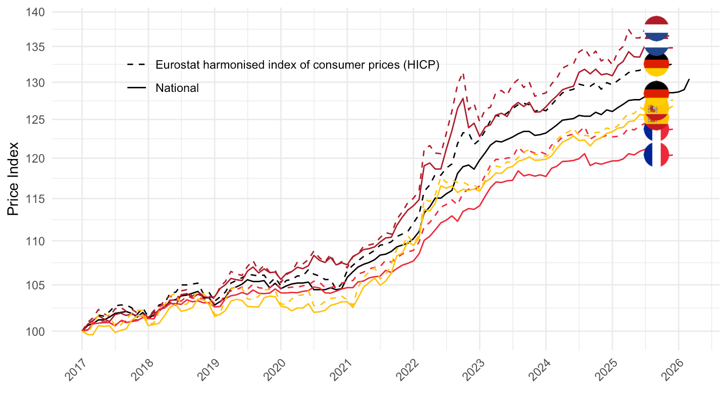
France vs. Germany vs. Italy vs. Netherlands vs. Spain
2017-
Code
PRICES_ALL %>%

  filter(EXPENDITURE == "_T",
         REF_AREA %in% c("FRA", "ESP", "CHE", "DEU"),
         ADJUSTMENT == "N",
         MEASURE == "CPI",
         TRANSFORMATION == "_Z",
         FREQ == "M") %>%
  month_to_date() %>%
  filter(date >= as.Date("2017-01-01")) %>%
  group_by(Ref_area, Methodology) %>%
  arrange(date) %>%
  mutate(obsValue = 100*obsValue/obsValue[1]) %>%
  left_join(colors, by = c("Ref_area"  = "country")) %>%
  ggplot(.) + geom_line(aes(x = date, y = obsValue, color = color, linetype = Methodology)) +
  scale_color_identity() +
  scale_linetype_manual(values = c("dashed", "solid")) + add_flags +
  theme_minimal() + xlab("") + ylab("Price Index") +
  scale_x_date(breaks = seq(1960, 2100, 1) %>% paste0("-01-01") %>% as.Date,
               labels = date_format("%Y")) +
  theme(legend.position = c(0.35, 0.8),
        legend.title = element_blank(),
        axis.text.x = element_text(angle = 45, vjust = 1, hjust = 1)) +
  scale_y_log10(breaks = seq(10, 200, 5))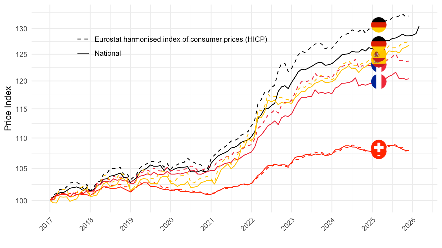
France vs. Germany
1996-
Code
PRICES_ALL %>%

  filter(EXPENDITURE == "_T",
         REF_AREA %in% c("FRA", "DEU"),
         ADJUSTMENT == "N",
         MEASURE == "CPI",
         TRANSFORMATION == "_Z",
         FREQ == "M") %>%
  month_to_date() %>%
  filter(date >= as.Date("1996-01-01")) %>%
  group_by(Ref_area, Methodology) %>%
  arrange(date) %>%
  mutate(obsValue = 100*obsValue/obsValue[1]) %>%
  left_join(colors, by = c("Ref_area"  = "country")) %>%
  ggplot(.) + geom_line(aes(x = date, y = obsValue, color = color, linetype = Methodology)) +
  scale_color_identity() +
  scale_linetype_manual(values = c("dashed", "solid")) + add_flags +
  theme_minimal() + xlab("") + ylab("Price Index") +
  scale_x_date(breaks = seq(1960, 2100, 1) %>% paste0("-01-01") %>% as.Date,
               labels = date_format("%Y")) +
  theme(legend.position = c(0.35, 0.8),
        legend.title = element_blank(),
        axis.text.x = element_text(angle = 45, vjust = 1, hjust = 1)) +
  scale_y_log10(breaks = seq(10, 200, 5))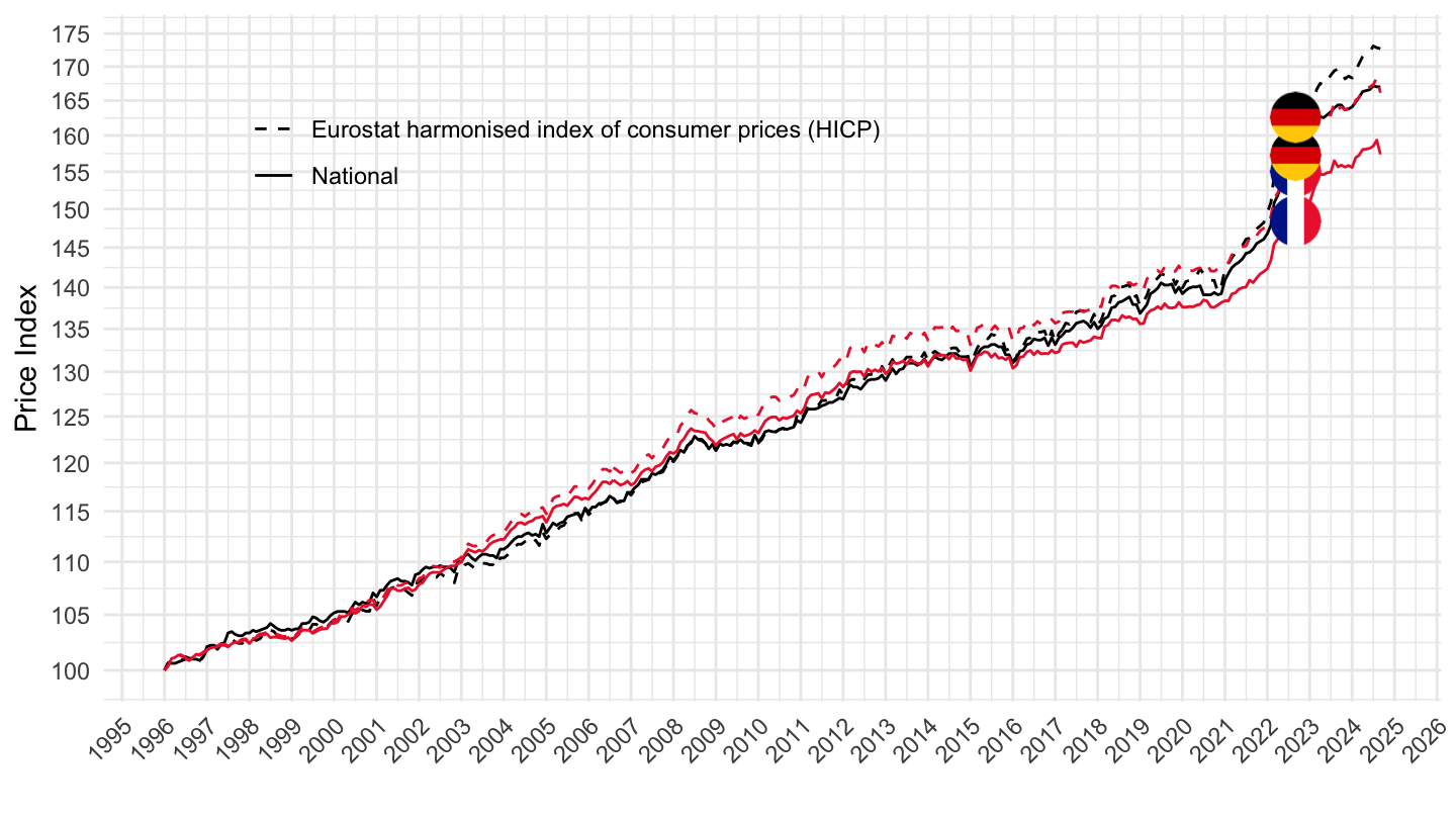
1999-
Code
PRICES_ALL %>%

  filter(EXPENDITURE == "_T",
         REF_AREA %in% c("FRA", "DEU"),
         ADJUSTMENT == "N",
         MEASURE == "CPI",
         TRANSFORMATION == "_Z",
         FREQ == "M") %>%
  month_to_date() %>%
  filter(date >= as.Date("1999-01-01")) %>%
  group_by(Ref_area, Methodology) %>%
  arrange(date) %>%
  mutate(obsValue = 100*obsValue/obsValue[1]) %>%
  left_join(colors, by = c("Ref_area"  = "country")) %>%
  ggplot(.) + geom_line(aes(x = date, y = obsValue, color = color, linetype = Methodology)) +
  scale_color_identity() +
  scale_linetype_manual(values = c("dashed", "solid")) + add_flags +
  theme_minimal() + xlab("") + ylab("Price Index") +
  scale_x_date(breaks = seq(1960, 2100, 1) %>% paste0("-01-01") %>% as.Date,
               labels = date_format("%Y")) +
  theme(legend.position = c(0.35, 0.8),
        legend.title = element_blank(),
        axis.text.x = element_text(angle = 45, vjust = 1, hjust = 1)) +
  scale_y_log10(breaks = seq(10, 200, 5))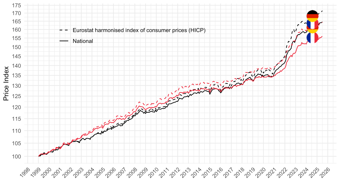
2017-
Code
PRICES_ALL %>%

  filter(EXPENDITURE == "_T",
         REF_AREA %in% c("FRA", "DEU"),
         ADJUSTMENT == "N",
         MEASURE == "CPI",
         TRANSFORMATION == "_Z",
         FREQ == "M") %>%
  month_to_date() %>%
  filter(date >= as.Date("2017-01-01")) %>%
  group_by(Ref_area, Methodology) %>%
  arrange(date) %>%
  mutate(obsValue = 100*obsValue/obsValue[1]) %>%
  left_join(colors, by = c("Ref_area"  = "country")) %>%
  ggplot(.) + geom_line(aes(x = date, y = obsValue, color = color, linetype = Methodology)) +
  scale_color_identity() +
  scale_linetype_manual(values = c("dashed", "solid")) + add_flags +
  theme_minimal() + xlab("") + ylab("Price Index") +
  scale_x_date(breaks = seq(1960, 2100, 1) %>% paste0("-01-01") %>% as.Date,
               labels = date_format("%Y")) +
  theme(legend.position = c(0.35, 0.8),
        legend.title = element_blank(),
        axis.text.x = element_text(angle = 45, vjust = 1, hjust = 1)) +
  scale_y_log10(breaks = seq(10, 200, 5))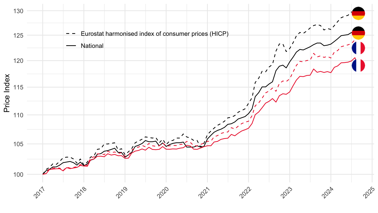
France vs. USA
CP041 - rents
1996-
Code
PRICES_ALL %>%

  filter(EXPENDITURE == "CP041",
         REF_AREA %in% c("FRA", "USA"),
         ADJUSTMENT == "N",
         MEASURE == "CPI",
         TRANSFORMATION == "_Z",
         FREQ == "M") %>%
  month_to_date() %>%
  filter(date >= as.Date("1996-01-01")) %>%
  group_by(Ref_area, Methodology) %>%
  arrange(date) %>%
  mutate(obsValue = 100*obsValue/obsValue[1]) %>%
  left_join(colors, by = c("Ref_area"  = "country")) %>%
  ggplot(.) + geom_line(aes(x = date, y = obsValue, color = color, linetype = Methodology)) +
  scale_color_identity() +
  scale_linetype_manual(values = c("dashed", "solid")) + add_flags +
  theme_minimal() + xlab("") + ylab("Price Index (CP041)") +
  scale_x_date(breaks = seq(1960, 2100, 1) %>% paste0("-01-01") %>% as.Date,
               labels = date_format("%Y")) +
  theme(legend.position = c(0.35, 0.8),
        legend.title = element_blank(),
        axis.text.x = element_text(angle = 45, vjust = 1, hjust = 1)) +
  scale_y_log10(breaks = seq(10, 200, 5))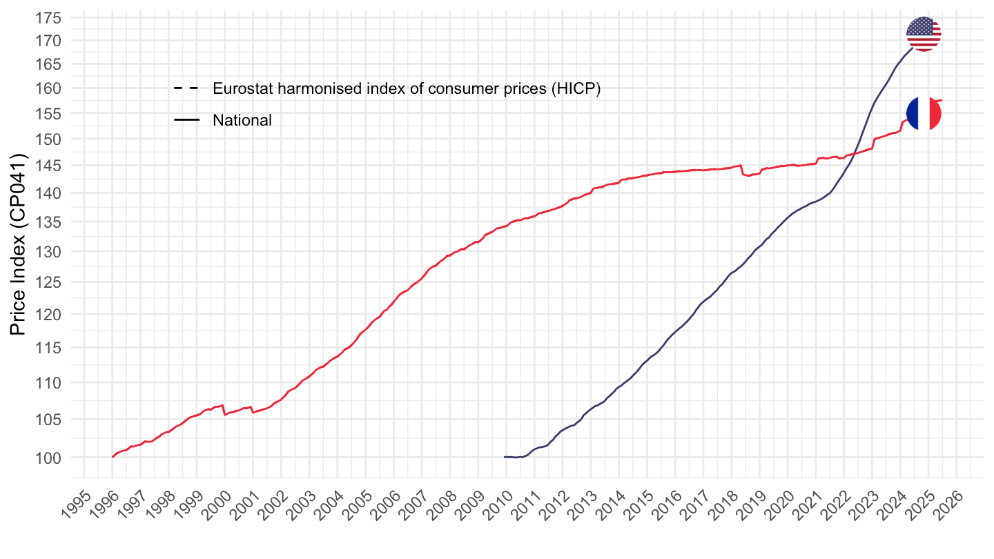
2002-
Code
PRICES_ALL %>%
  filter(EXPENDITURE == "CP041",
         REF_AREA %in% c("FRA", "USA"),
         ADJUSTMENT == "N",
         MEASURE == "CPI",
         TRANSFORMATION == "_Z",
         FREQ == "M") %>%


  month_to_date() %>%
  filter(date >= as.Date("2002-01-01")) %>%
  group_by(Ref_area, Methodology) %>%
  arrange(date) %>%
  mutate(obsValue = 100*obsValue/obsValue[1]) %>%
  left_join(colors, by = c("Ref_area"  = "country")) %>%
  ggplot(.) + geom_line(aes(x = date, y = obsValue, color = color, linetype = Methodology)) +
  scale_color_identity() +
  scale_linetype_manual(values = c("dashed", "solid")) + add_flags +
  theme_minimal() + xlab("") + ylab("Price Index (CP041)") +
  scale_x_date(breaks = seq(1960, 2100, 1) %>% paste0("-01-01") %>% as.Date,
               labels = date_format("%Y")) +
  theme(legend.position = c(0.35, 0.2),
        legend.title = element_blank(),
        axis.text.x = element_text(angle = 45, vjust = 1, hjust = 1)) +
  scale_y_log10(breaks = seq(10, 200, 5))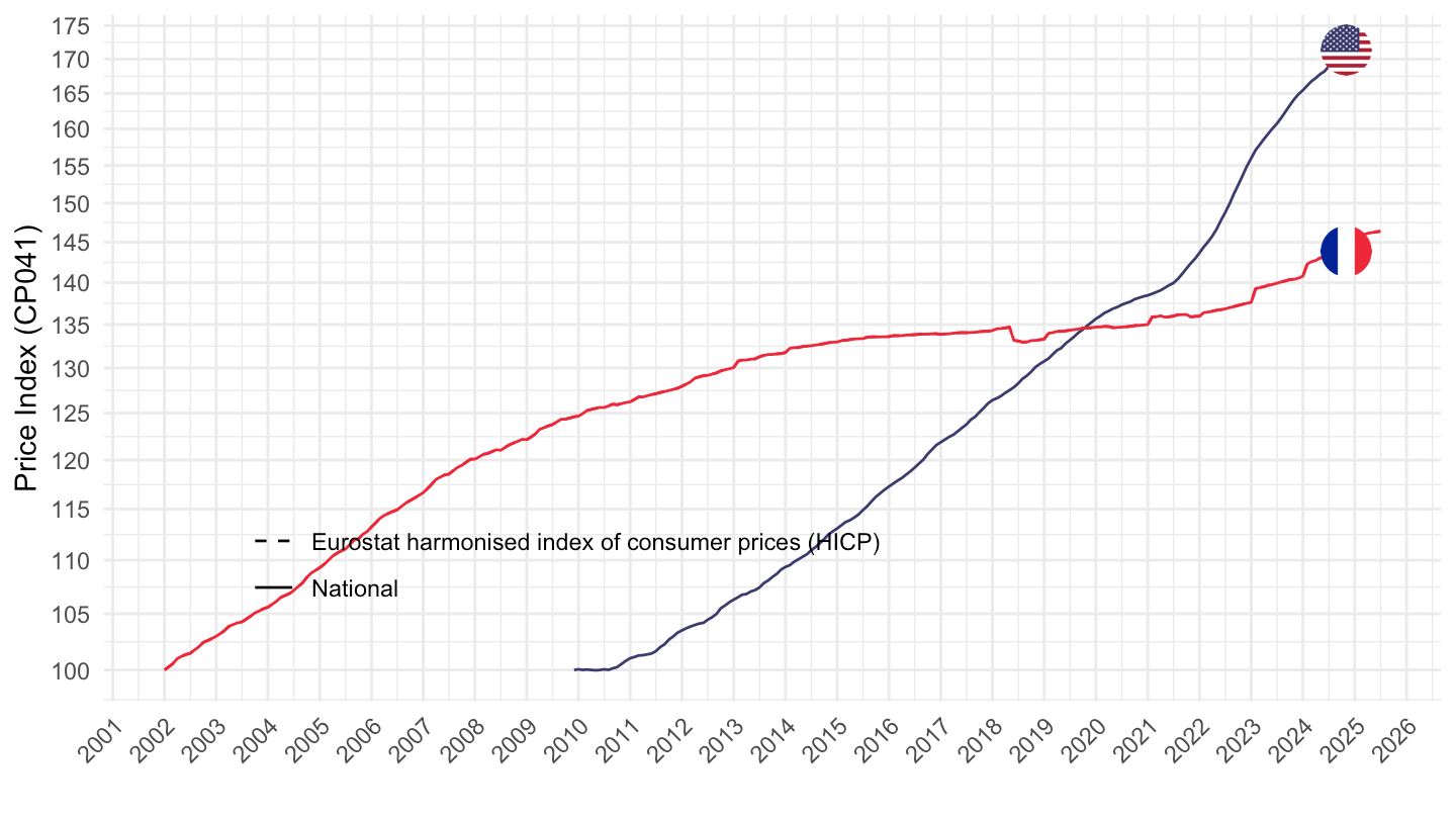
2010-
Code
PRICES_ALL %>%
  filter(EXPENDITURE == "CP041",
         REF_AREA %in% c("FRA", "USA"),
         ADJUSTMENT == "N",
         MEASURE == "CPI",
         TRANSFORMATION == "_Z",
         FREQ == "M") %>%


  month_to_date() %>%
  filter(date >= as.Date("2010-01-01")) %>%
  group_by(Ref_area, Methodology) %>%
  arrange(date) %>%
  mutate(obsValue = 100*obsValue/obsValue[1]) %>%
  left_join(colors, by = c("Ref_area"  = "country")) %>%
  ggplot(.) + geom_line(aes(x = date, y = obsValue, color = color, linetype = Methodology)) +
  scale_color_identity() +
  scale_linetype_manual(values = c("dashed", "solid")) + add_flags +
  theme_minimal() + xlab("") + ylab("Price Index (CP041)") +
  scale_x_date(breaks = seq(1960, 2100, 1) %>% paste0("-01-01") %>% as.Date,
               labels = date_format("%Y")) +
  theme(legend.position = c(0.35, 0.2),
        legend.title = element_blank(),
        axis.text.x = element_text(angle = 45, vjust = 1, hjust = 1)) +
  scale_y_log10(breaks = seq(10, 200, 5))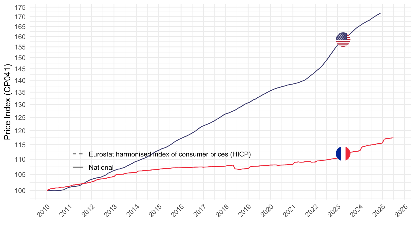
2017-
Code
PRICES_ALL %>%

  filter(EXPENDITURE == "CP041",
         REF_AREA %in% c("FRA", "USA"),
         ADJUSTMENT == "N",
         MEASURE == "CPI",
         TRANSFORMATION == "_Z",
         FREQ == "M") %>%
  month_to_date() %>%
  filter(date >= as.Date("2017-01-01")) %>%
  group_by(Ref_area, Methodology) %>%
  arrange(date) %>%
  mutate(obsValue = 100*obsValue/obsValue[1]) %>%
  left_join(colors, by = c("Ref_area"  = "country")) %>%
  ggplot(.) + geom_line(aes(x = date, y = obsValue, color = color, linetype = Methodology)) +
  scale_color_identity() +
  scale_linetype_manual(values = c("dashed", "solid")) + add_flags +
  theme_minimal() + xlab("") + ylab("Price Index (CP041)") +
  scale_x_date(breaks = seq(1960, 2100, 1) %>% paste0("-01-01") %>% as.Date,
               labels = date_format("%Y")) +
  theme(legend.position = c(0.35, 0.8),
        legend.title = element_blank(),
        axis.text.x = element_text(angle = 45, vjust = 1, hjust = 1)) +
  scale_y_log10(breaks = seq(10, 200, 5))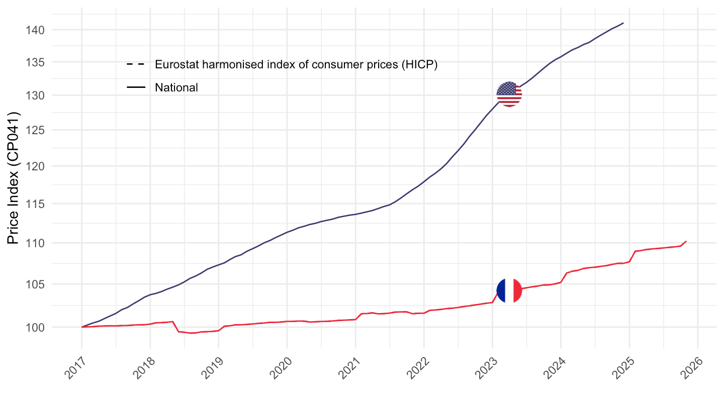
GD
1996-
Code
PRICES_ALL %>%
  filter(EXPENDITURE == "GD",
         REF_AREA %in% c("FRA", "USA"),
         ADJUSTMENT == "N",
         MEASURE == "CPI",
         TRANSFORMATION == "_Z",
         FREQ == "M") %>%


  month_to_date() %>%
  filter(date >= as.Date("1996-01-01")) %>%
  group_by(Ref_area, Methodology) %>%
  arrange(date) %>%
  mutate(obsValue = 100*obsValue/obsValue[1]) %>%
  left_join(colors, by = c("Ref_area"  = "country")) %>%
  ggplot(.) + geom_line(aes(x = date, y = obsValue, color = color, linetype = Methodology)) +
  scale_color_identity() +
  scale_linetype_manual(values = c("dashed", "solid")) + add_flags +
  theme_minimal() + xlab("") + ylab("Price Index (CP09)") +
  scale_x_date(breaks = seq(1960, 2100, 1) %>% paste0("-01-01") %>% as.Date,
               labels = date_format("%Y")) +
  theme(legend.position = c(0.35, 0.8),
        legend.title = element_blank(),
        axis.text.x = element_text(angle = 45, vjust = 1, hjust = 1)) +
  scale_y_log10(breaks = seq(10, 200, 5))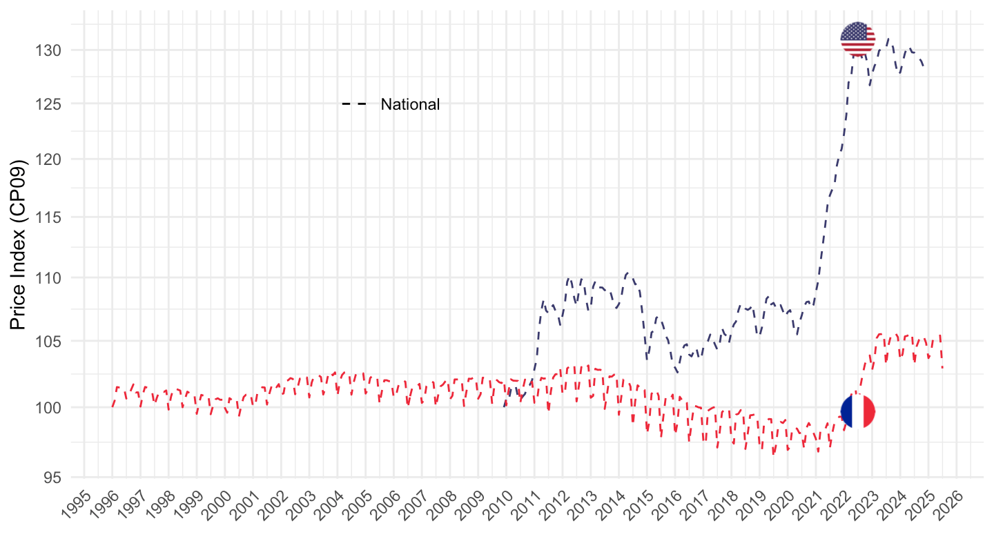
2002-
Code
PRICES_ALL %>%
  filter(EXPENDITURE == "GD",
         REF_AREA %in% c("FRA", "USA"),
         ADJUSTMENT == "N",
         MEASURE == "CPI",
         TRANSFORMATION == "_Z",
         FREQ == "M") %>%


  month_to_date() %>%
  filter(date >= as.Date("2002-01-01")) %>%
  group_by(Ref_area, Methodology) %>%
  arrange(date) %>%
  mutate(obsValue = 100*obsValue/obsValue[1]) %>%
  left_join(colors, by = c("Ref_area"  = "country")) %>%
  ggplot(.) + geom_line(aes(x = date, y = obsValue, color = color, linetype = Methodology)) +
  scale_color_identity() +
  scale_linetype_manual(values = c("dashed", "solid")) + add_flags +
  theme_minimal() + xlab("") + ylab("Price Index (CP09)") +
  scale_x_date(breaks = seq(1960, 2100, 1) %>% paste0("-01-01") %>% as.Date,
               labels = date_format("%Y")) +
  theme(legend.position = c(0.35, 0.2),
        legend.title = element_blank(),
        axis.text.x = element_text(angle = 45, vjust = 1, hjust = 1)) +
  scale_y_log10(breaks = seq(10, 200, 5))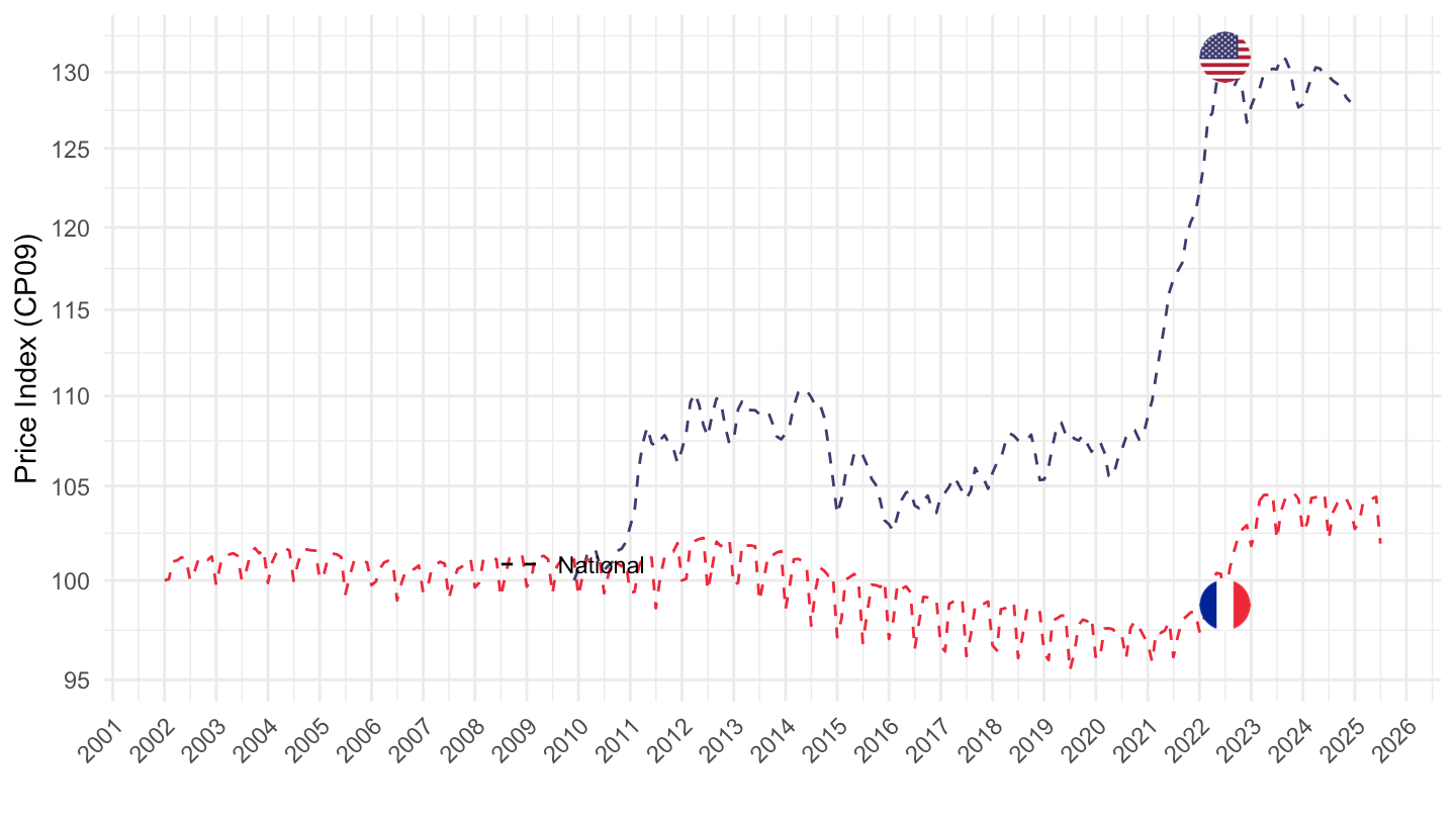
2017-
Code
PRICES_ALL %>%
  filter(EXPENDITURE == "GD",
         REF_AREA %in% c("FRA", "USA"),
         ADJUSTMENT == "N",
         MEASURE == "CPI",
         TRANSFORMATION == "_Z",
         FREQ == "M") %>%


  month_to_date() %>%
  filter(date >= as.Date("2017-01-01")) %>%
  group_by(Ref_area, Methodology) %>%
  arrange(date) %>%
  mutate(obsValue = 100*obsValue/obsValue[1]) %>%
  left_join(colors, by = c("Ref_area"  = "country")) %>%
  ggplot(.) + geom_line(aes(x = date, y = obsValue, color = color)) +
  scale_color_identity() +
  scale_linetype_manual(values = c("dashed", "solid")) + add_flags +
  theme_minimal() + xlab("") + ylab("Price Index (GD)") +
  scale_x_date(breaks = seq(1960, 2100, 1) %>% paste0("-01-01") %>% as.Date,
               labels = date_format("%Y")) +
  theme(legend.position = c(0.35, 0.2),
        legend.title = element_blank(),
        axis.text.x = element_text(angle = 45, vjust = 1, hjust = 1)) +
  scale_y_log10(breaks = seq(10, 200, 5))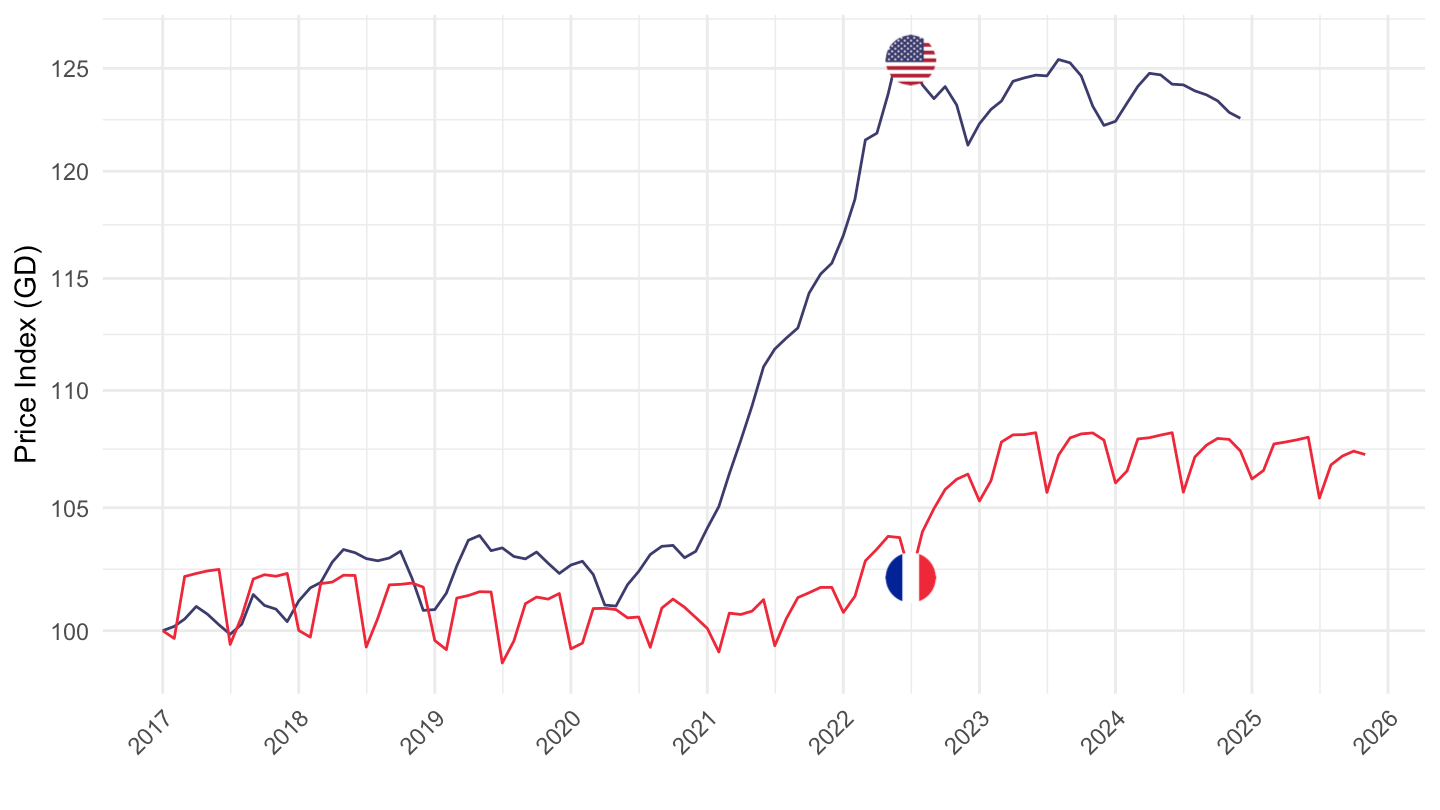
CP07
1996-
Code
PRICES_ALL %>%
  filter(EXPENDITURE == "CP07",
         REF_AREA %in% c("FRA", "USA"),
         ADJUSTMENT == "N",
         MEASURE == "CPI",
         TRANSFORMATION == "_Z",
         FREQ == "M") %>%


  month_to_date() %>%
  filter(date >= as.Date("1996-01-01")) %>%
  group_by(Ref_area, Methodology) %>%
  arrange(date) %>%
  mutate(obsValue = 100*obsValue/obsValue[1]) %>%
  left_join(colors, by = c("Ref_area"  = "country")) %>%
  ggplot(.) + geom_line(aes(x = date, y = obsValue, color = color, linetype = Methodology)) +
  scale_color_identity() +
  scale_linetype_manual(values = c("dashed", "solid")) + add_flags +
  theme_minimal() + xlab("") + ylab("Price Index (CP09)") +
  scale_x_date(breaks = seq(1960, 2100, 1) %>% paste0("-01-01") %>% as.Date,
               labels = date_format("%Y")) +
  theme(legend.position = c(0.35, 0.8),
        legend.title = element_blank(),
        axis.text.x = element_text(angle = 45, vjust = 1, hjust = 1)) +
  scale_y_log10(breaks = seq(10, 200, 5))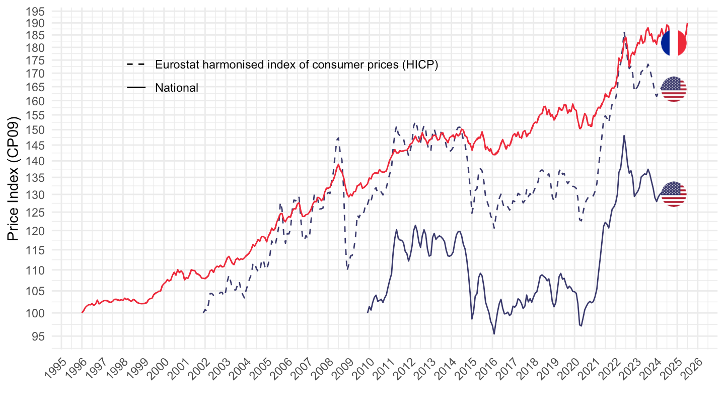
2002-
Code
PRICES_ALL %>%
  filter(EXPENDITURE == "CP07",
         REF_AREA %in% c("FRA", "USA"),
         ADJUSTMENT == "N",
         MEASURE == "CPI",
         TRANSFORMATION == "_Z",
         FREQ == "M") %>%


  month_to_date() %>%
  filter(date >= as.Date("2002-01-01")) %>%
  group_by(Ref_area, Methodology) %>%
  arrange(date) %>%
  mutate(obsValue = 100*obsValue/obsValue[1]) %>%
  left_join(colors, by = c("Ref_area"  = "country")) %>%
  ggplot(.) + geom_line(aes(x = date, y = obsValue, color = color, linetype = Methodology)) +
  scale_color_identity() +
  scale_linetype_manual(values = c("dashed", "solid")) + add_flags +
  theme_minimal() + xlab("") + ylab("Price Index (CP09)") +
  scale_x_date(breaks = seq(1960, 2100, 1) %>% paste0("-01-01") %>% as.Date,
               labels = date_format("%Y")) +
  theme(legend.position = c(0.35, 0.2),
        legend.title = element_blank(),
        axis.text.x = element_text(angle = 45, vjust = 1, hjust = 1)) +
  scale_y_log10(breaks = seq(10, 200, 5))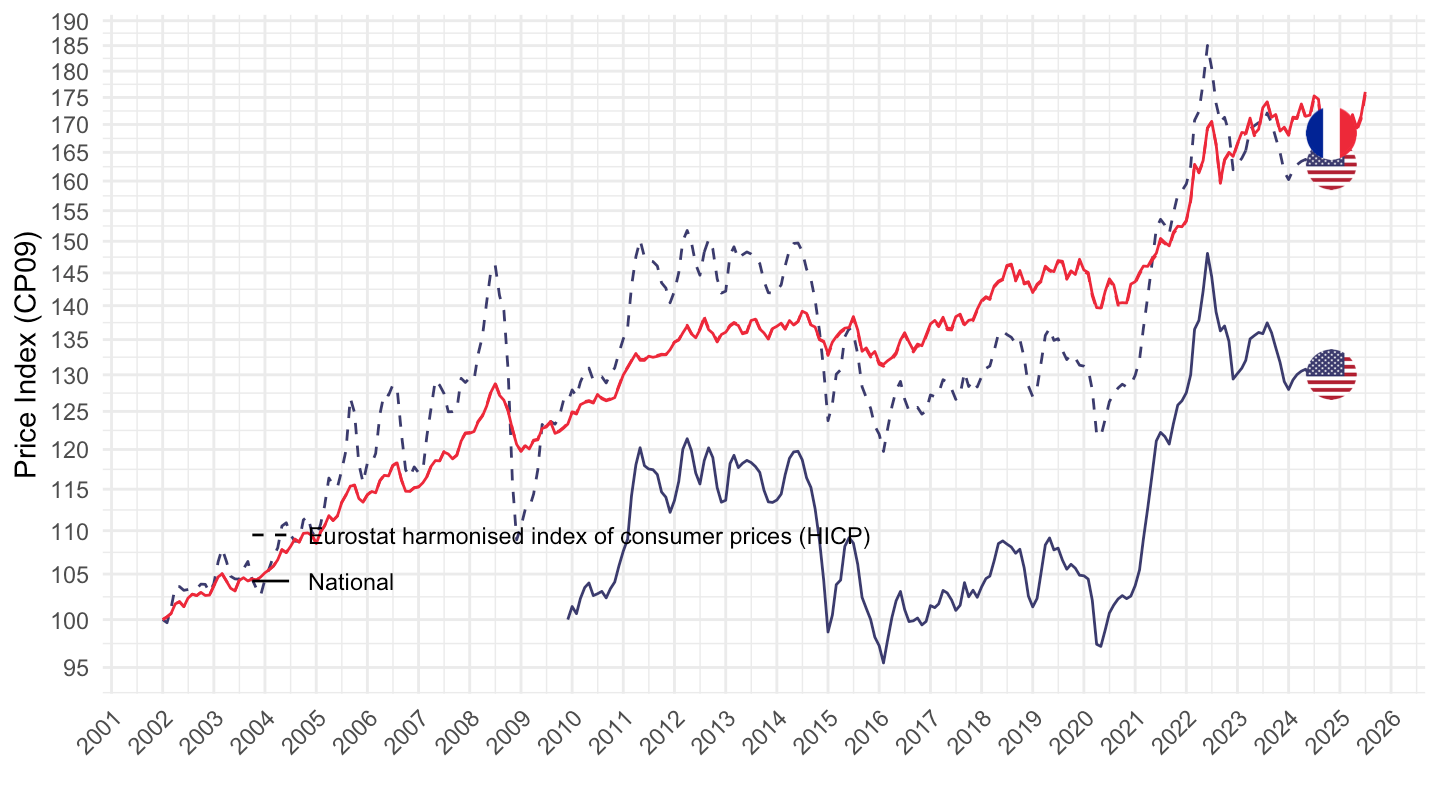
2017-
Code
PRICES_ALL %>%
  filter(EXPENDITURE == "CP07",
         REF_AREA %in% c("FRA", "USA"),
         ADJUSTMENT == "N",
         MEASURE == "CPI",
         TRANSFORMATION == "_Z",
         FREQ == "M") %>%


  month_to_date() %>%
  filter(date >= as.Date("2017-01-01")) %>%
  group_by(Ref_area, Methodology) %>%
  arrange(date) %>%
  mutate(obsValue = 100*obsValue/obsValue[1]) %>%
  left_join(colors, by = c("Ref_area"  = "country")) %>%
  ggplot(.) + geom_line(aes(x = date, y = obsValue, color = color, linetype = Methodology)) +
  scale_color_identity() +
  scale_linetype_manual(values = c("dashed", "solid")) + add_flags +
  theme_minimal() + xlab("") + ylab("Price Index (CP07)") +
  scale_x_date(breaks = seq(1960, 2100, 1) %>% paste0("-01-01") %>% as.Date,
               labels = date_format("%Y")) +
  theme(legend.position = c(0.35, 0.2),
        legend.title = element_blank(),
        axis.text.x = element_text(angle = 45, vjust = 1, hjust = 1)) +
  scale_y_log10(breaks = seq(10, 200, 5))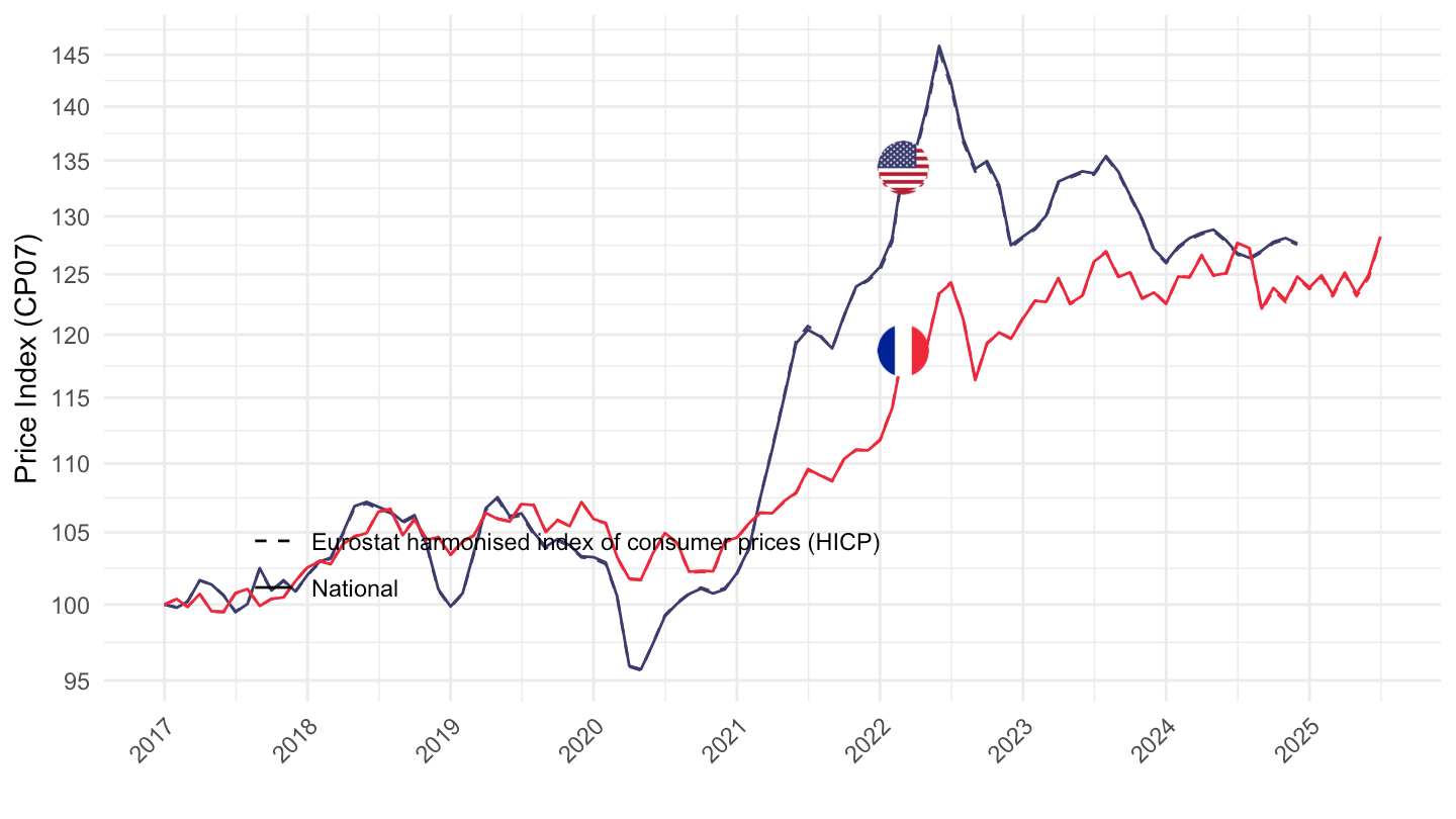
2020-
Code
PRICES_ALL %>%
  filter(EXPENDITURE == "CP07",
         REF_AREA %in% c("FRA", "USA"),
         ADJUSTMENT == "N",
         MEASURE == "CPI",
         TRANSFORMATION == "_Z",
         FREQ == "M") %>%


  month_to_date() %>%
  filter(date >= as.Date("2020-01-01")) %>%
  group_by(Ref_area, Methodology) %>%
  arrange(date) %>%
  mutate(obsValue = 100*obsValue/obsValue[1]) %>%
  left_join(colors, by = c("Ref_area"  = "country")) %>%
  ggplot(.) + geom_line(aes(x = date, y = obsValue, color = color, linetype = Methodology)) +
  scale_color_identity() +
  scale_linetype_manual(values = c("dashed", "solid")) + add_flags +
  theme_minimal() + xlab("") + ylab("Price Index (CP07)") +
  scale_x_date(breaks = seq(1960, 2100, 1) %>% paste0("-01-01") %>% as.Date,
               labels = date_format("%Y")) +
  theme(legend.position = c(0.35, 0.2),
        legend.title = element_blank(),
        axis.text.x = element_text(angle = 45, vjust = 1, hjust = 1)) +
  scale_y_log10(breaks = seq(10, 200, 5))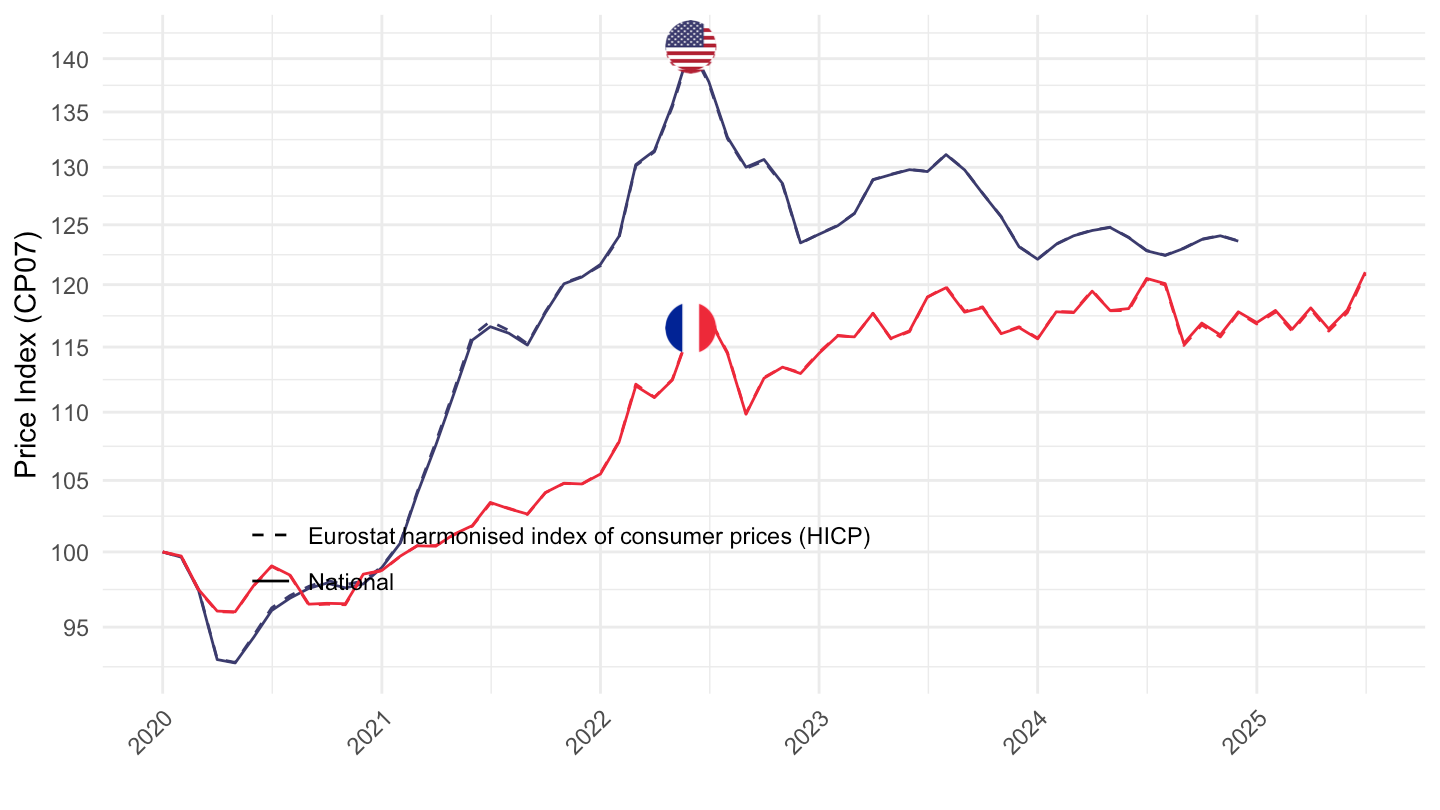
CP09
1996-
Code
PRICES_ALL %>%
  filter(EXPENDITURE == "CP09",
         REF_AREA %in% c("FRA", "USA"),
         ADJUSTMENT == "N",
         MEASURE == "CPI",
         TRANSFORMATION == "_Z",
         FREQ == "M") %>%


  month_to_date() %>%
  filter(date >= as.Date("1996-01-01")) %>%
  group_by(Ref_area, Methodology) %>%
  arrange(date) %>%
  mutate(obsValue = 100*obsValue/obsValue[1]) %>%
  left_join(colors, by = c("Ref_area"  = "country")) %>%
  ggplot(.) + geom_line(aes(x = date, y = obsValue, color = color, linetype = Methodology)) +
  scale_color_identity() +
  scale_linetype_manual(values = c("dashed", "solid")) + add_flags +
  theme_minimal() + xlab("") + ylab("Price Index (CP09)") +
  scale_x_date(breaks = seq(1960, 2100, 1) %>% paste0("-01-01") %>% as.Date,
               labels = date_format("%Y")) +
  theme(legend.position = c(0.35, 0.8),
        legend.title = element_blank(),
        axis.text.x = element_text(angle = 45, vjust = 1, hjust = 1)) +
  scale_y_log10(breaks = seq(10, 200, 5))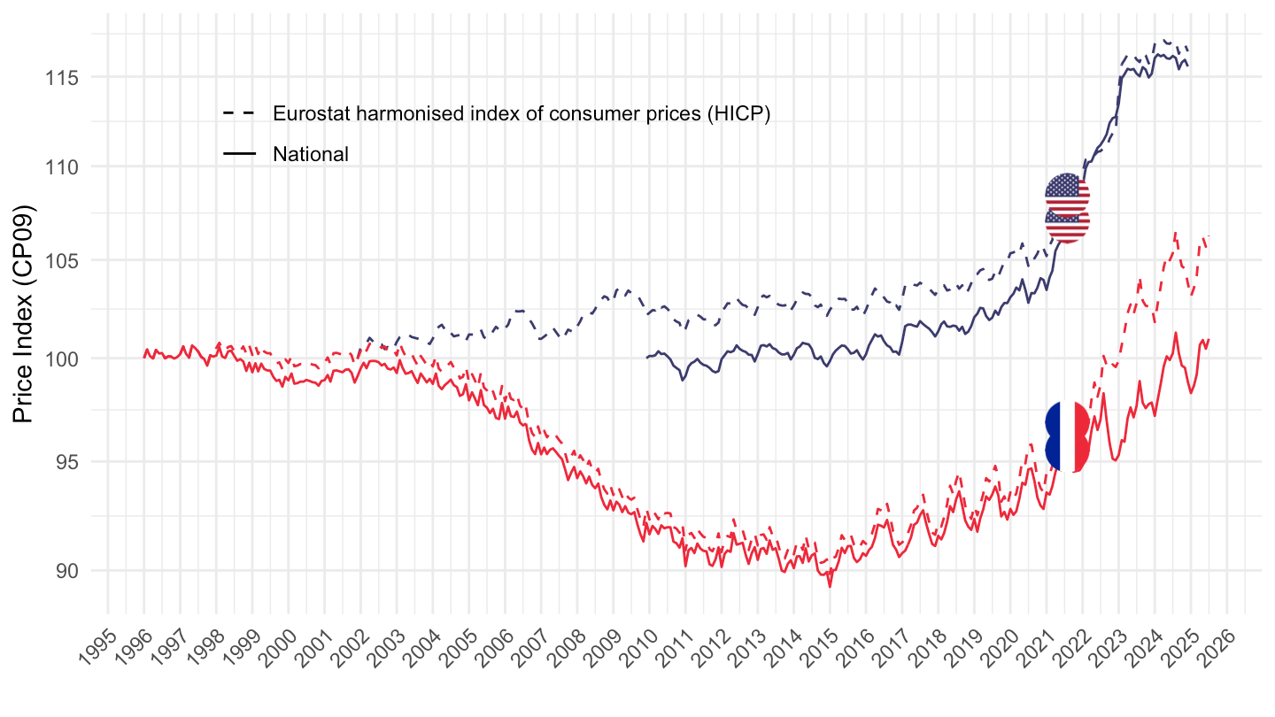
2002-
Code
PRICES_ALL %>%
  filter(EXPENDITURE == "CP09",
         REF_AREA %in% c("FRA", "USA"),
         ADJUSTMENT == "N",
         MEASURE == "CPI",
         TRANSFORMATION == "_Z",
         FREQ == "M") %>%


  month_to_date() %>%
  filter(date >= as.Date("2002-01-01")) %>%
  group_by(Ref_area, Methodology) %>%
  arrange(date) %>%
  mutate(obsValue = 100*obsValue/obsValue[1]) %>%
  left_join(colors, by = c("Ref_area"  = "country")) %>%
  ggplot(.) + geom_line(aes(x = date, y = obsValue, color = color, linetype = Methodology)) +
  scale_color_identity() +
  scale_linetype_manual(values = c("dashed", "solid")) + add_flags +
  theme_minimal() + xlab("") + ylab("Price Index (CP09)") +
  scale_x_date(breaks = seq(1960, 2100, 1) %>% paste0("-01-01") %>% as.Date,
               labels = date_format("%Y")) +
  theme(legend.position = c(0.35, 0.2),
        legend.title = element_blank(),
        axis.text.x = element_text(angle = 45, vjust = 1, hjust = 1)) +
  scale_y_log10(breaks = seq(10, 200, 5))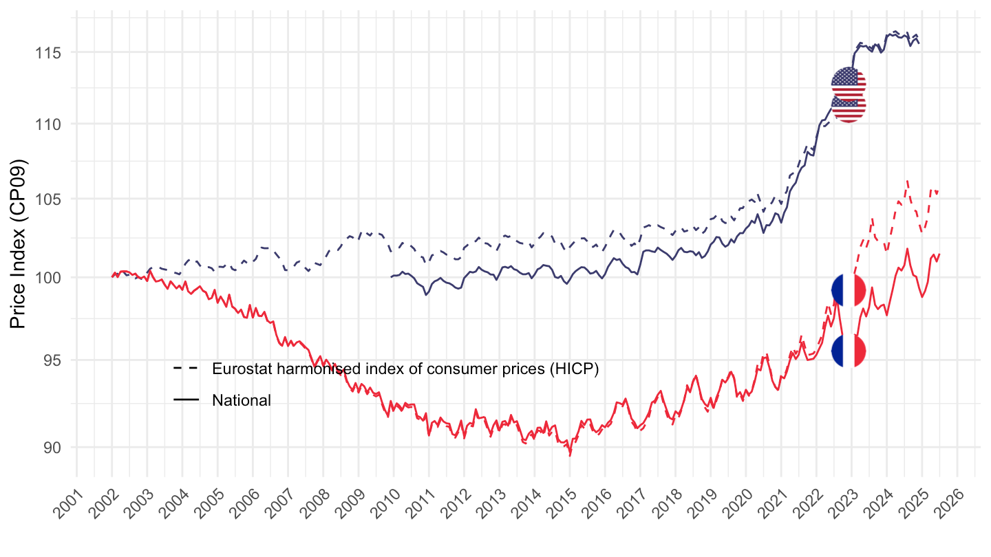
2017-
Code
PRICES_ALL %>%
  filter(EXPENDITURE == "CP09",
         REF_AREA %in% c("FRA", "USA"),
         ADJUSTMENT == "N",
         MEASURE == "CPI",
         TRANSFORMATION == "_Z",
         FREQ == "M") %>%


  month_to_date() %>%
  filter(date >= as.Date("2017-01-01")) %>%
  group_by(Ref_area, Methodology) %>%
  arrange(date) %>%
  mutate(obsValue = 100*obsValue/obsValue[1]) %>%
  left_join(colors, by = c("Ref_area"  = "country")) %>%
  ggplot(.) + geom_line(aes(x = date, y = obsValue, color = color, linetype = Methodology)) +
  scale_color_identity() +
  scale_linetype_manual(values = c("dashed", "solid")) + add_flags +
  theme_minimal() + xlab("") + ylab("Price Index (CP09)") +
  scale_x_date(breaks = seq(1960, 2100, 1) %>% paste0("-01-01") %>% as.Date,
               labels = date_format("%Y")) +
  theme(legend.position = c(0.35, 0.2),
        legend.title = element_blank(),
        axis.text.x = element_text(angle = 45, vjust = 1, hjust = 1)) +
  scale_y_log10(breaks = seq(10, 200, 5))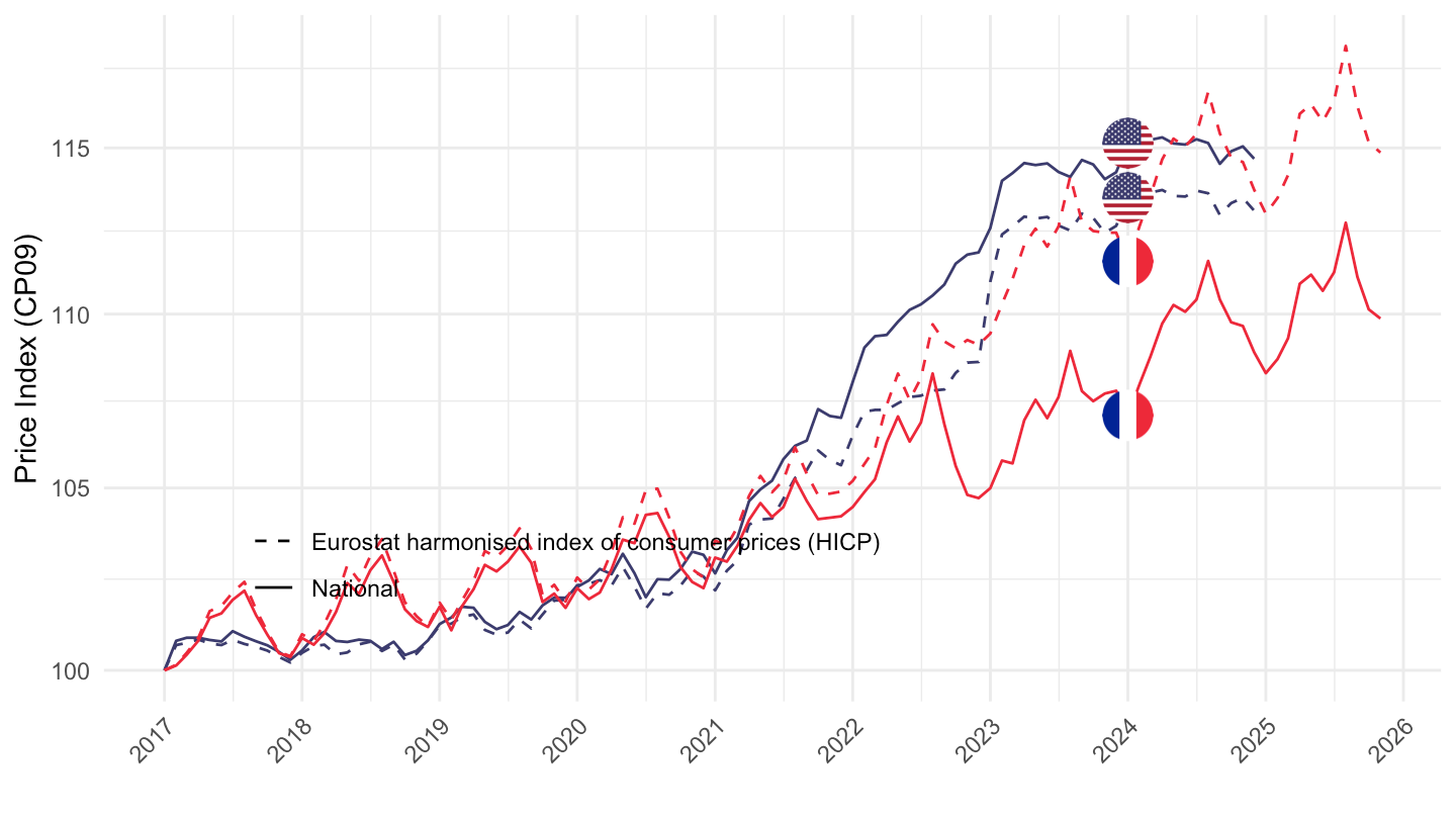
CP08
1996-
Code
PRICES_ALL %>%
  filter(EXPENDITURE == "CP08",
         REF_AREA %in% c("FRA", "USA"),
         ADJUSTMENT == "N",
         MEASURE == "CPI",
         TRANSFORMATION == "_Z",
         FREQ == "M") %>%


  month_to_date() %>%
  filter(date >= as.Date("1996-01-01")) %>%
  group_by(Ref_area, Methodology) %>%
  arrange(date) %>%
  mutate(obsValue = 100*obsValue/obsValue[1]) %>%
  left_join(colors, by = c("Ref_area"  = "country")) %>%
  ggplot(.) + geom_line(aes(x = date, y = obsValue, color = color, linetype = Methodology)) +
  scale_color_identity() +
  scale_linetype_manual(values = c("dashed", "solid")) + add_flags +
  theme_minimal() + xlab("") + ylab("Price Index (CP08)") +
  scale_x_date(breaks = seq(1960, 2100, 1) %>% paste0("-01-01") %>% as.Date,
               labels = date_format("%Y")) +
  theme(legend.position = c(0.35, 0.2),
        legend.title = element_blank(),
        axis.text.x = element_text(angle = 45, vjust = 1, hjust = 1)) +
  scale_y_log10(breaks = seq(10, 200, 5))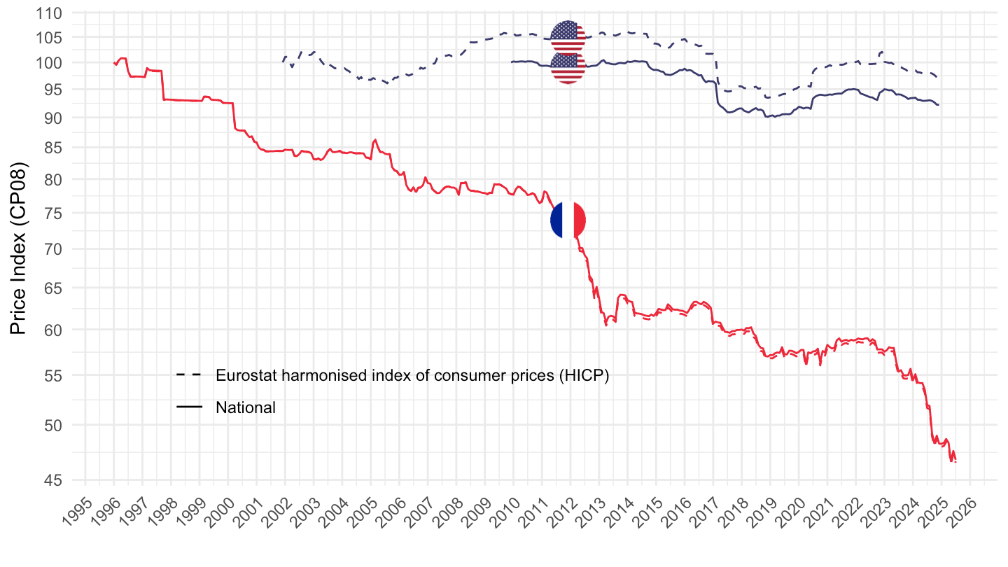
2002-
Code
PRICES_ALL %>%
  filter(EXPENDITURE == "CP08",
         REF_AREA %in% c("FRA", "USA"),
         ADJUSTMENT == "N",
         MEASURE == "CPI",
         TRANSFORMATION == "_Z",
         FREQ == "M") %>%


  month_to_date() %>%
  filter(date >= as.Date("2002-01-01")) %>%
  group_by(Ref_area, Methodology) %>%
  arrange(date) %>%
  mutate(obsValue = 100*obsValue/obsValue[1]) %>%
  left_join(colors, by = c("Ref_area"  = "country")) %>%
  ggplot(.) + geom_line(aes(x = date, y = obsValue, color = color, linetype = Methodology)) +
  scale_color_identity() +
  scale_linetype_manual(values = c("dashed", "solid")) + add_flags +
  theme_minimal() + xlab("") + ylab("Price Index (CP08)") +
  scale_x_date(breaks = seq(1960, 2100, 1) %>% paste0("-01-01") %>% as.Date,
               labels = date_format("%Y")) +
  theme(legend.position = c(0.35, 0.2),
        legend.title = element_blank(),
        axis.text.x = element_text(angle = 45, vjust = 1, hjust = 1)) +
  scale_y_log10(breaks = seq(10, 200, 5))
2017-
Code
PRICES_ALL %>%
  filter(EXPENDITURE == "CP08",
         REF_AREA %in% c("FRA", "USA"),
         ADJUSTMENT == "N",
         MEASURE == "CPI",
         TRANSFORMATION == "_Z",
         FREQ == "M") %>%


  month_to_date() %>%
  filter(date >= as.Date("2017-01-01")) %>%
  group_by(Ref_area, Methodology) %>%
  arrange(date) %>%
  mutate(obsValue = 100*obsValue/obsValue[1]) %>%
  left_join(colors, by = c("Ref_area"  = "country")) %>%
  ggplot(.) + geom_line(aes(x = date, y = obsValue, color = color, linetype = Methodology)) +
  scale_color_identity() +
  scale_linetype_manual(values = c("dashed", "solid")) + add_flags +
  theme_minimal() + xlab("") + ylab("Price Index (CP08)") +
  scale_x_date(breaks = seq(1960, 2100, 1) %>% paste0("-01-01") %>% as.Date,
               labels = date_format("%Y")) +
  theme(legend.position = c(0.35, 0.2),
        legend.title = element_blank(),
        axis.text.x = element_text(angle = 45, vjust = 1, hjust = 1)) +
  scale_y_log10(breaks = seq(10, 200, 5))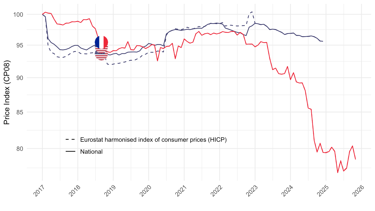
All
1996-
Code
PRICES_ALL %>%
  filter(EXPENDITURE == "_T",
         REF_AREA %in% c("FRA", "USA"),
         ADJUSTMENT == "N",
         MEASURE == "CPI",
         TRANSFORMATION == "_Z",
         FREQ == "M") %>%


  month_to_date() %>%
  filter(date >= as.Date("1996-01-01")) %>%
  group_by(Ref_area, Methodology) %>%
  arrange(date) %>%
  mutate(obsValue = 100*obsValue/obsValue[1]) %>%
  left_join(colors, by = c("Ref_area"  = "country")) %>%
  ggplot(.) + geom_line(aes(x = date, y = obsValue, color = color, linetype = Methodology)) +
  scale_color_identity() +
  scale_linetype_manual(values = c("dashed", "solid")) + add_flags +
  theme_minimal() + xlab("") + ylab("Price Index") +
  scale_x_date(breaks = seq(1960, 2100, 1) %>% paste0("-01-01") %>% as.Date,
               labels = date_format("%Y")) +
  theme(legend.position = c(0.35, 0.8),
        legend.title = element_blank(),
        axis.text.x = element_text(angle = 45, vjust = 1, hjust = 1)) +
  scale_y_log10(breaks = seq(10, 200, 5))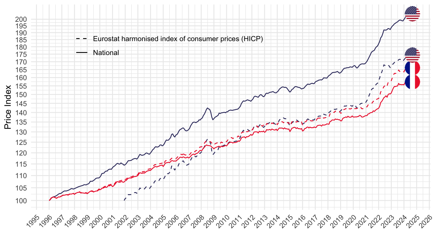
2002-
Code
PRICES_ALL %>%
  filter(EXPENDITURE == "_T",
         REF_AREA %in% c("FRA", "USA"),
         ADJUSTMENT == "N",
         MEASURE == "CPI",
         TRANSFORMATION == "_Z",
         FREQ == "M") %>%


  month_to_date() %>%
  filter(date >= as.Date("2002-01-01")) %>%
  group_by(Ref_area, Methodology) %>%
  arrange(date) %>%
  mutate(obsValue = 100*obsValue/obsValue[1]) %>%
  left_join(colors, by = c("Ref_area"  = "country")) %>%
  ggplot(.) + geom_line(aes(x = date, y = obsValue, color = color, linetype = Methodology)) +
  scale_color_identity() +
  scale_linetype_manual(values = c("dashed", "solid")) + add_flags +
  theme_minimal() + xlab("") + ylab("Price Index") +
  scale_x_date(breaks = seq(1960, 2100, 1) %>% paste0("-01-01") %>% as.Date,
               labels = date_format("%Y")) +
  theme(legend.position = c(0.35, 0.8),
        legend.title = element_blank(),
        axis.text.x = element_text(angle = 45, vjust = 1, hjust = 1)) +
  scale_y_log10(breaks = seq(10, 200, 5))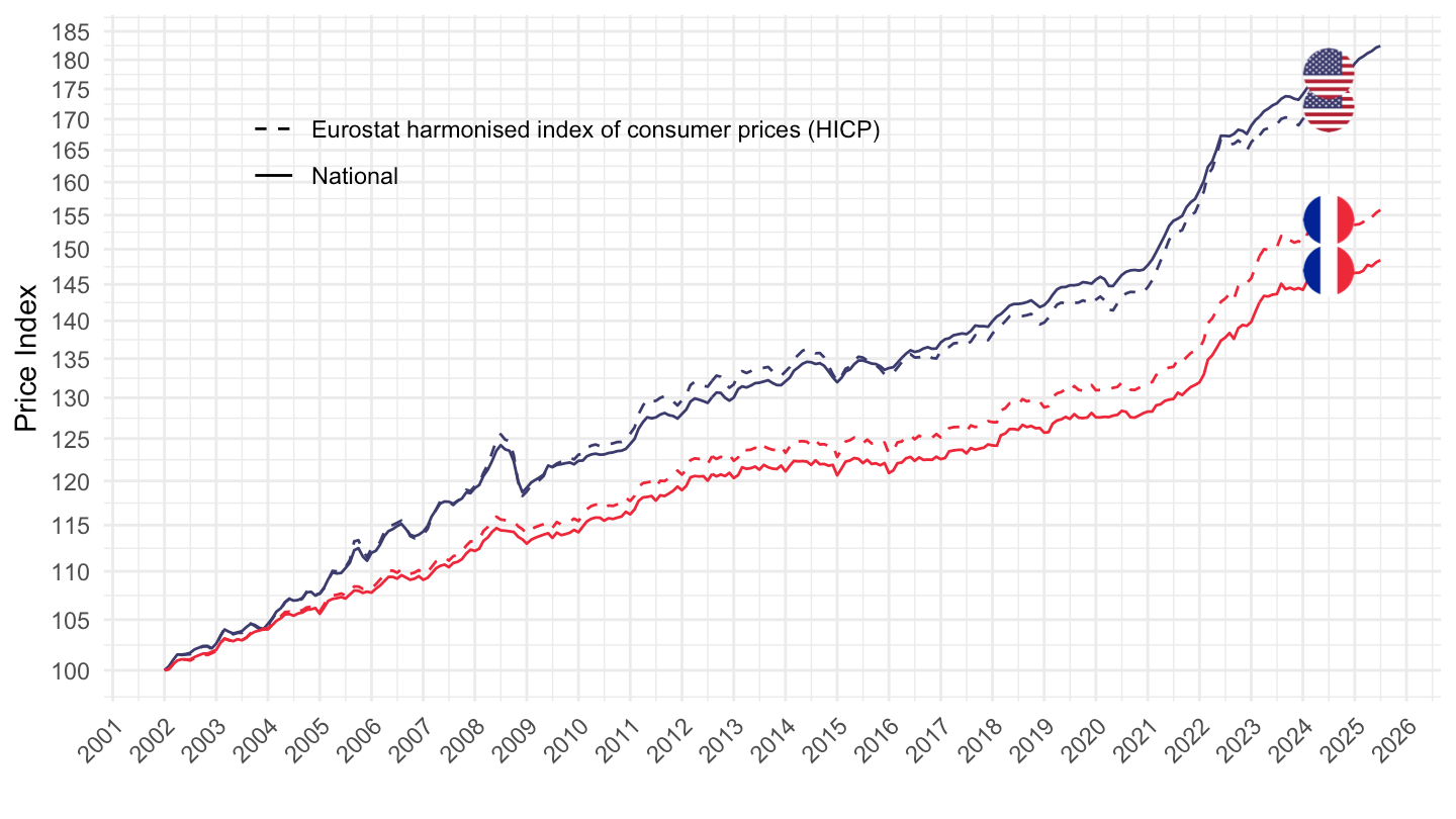
2017-
Code
PRICES_ALL %>%
  filter(EXPENDITURE == "_T",
         REF_AREA %in% c("FRA", "USA"),
         ADJUSTMENT == "N",
         MEASURE == "CPI",
         TRANSFORMATION == "_Z",
         FREQ == "M") %>%


  month_to_date() %>%
  filter(date >= as.Date("2017-01-01")) %>%
  group_by(Ref_area, Methodology) %>%
  arrange(date) %>%
  mutate(obsValue = 100*obsValue/obsValue[1]) %>%
  left_join(colors, by = c("Ref_area"  = "country")) %>%
  ggplot(.) + geom_line(aes(x = date, y = obsValue, color = color, linetype = Methodology)) +
  scale_color_identity() +
  scale_linetype_manual(values = c("dashed", "solid")) + add_flags +
  theme_minimal() + xlab("") + ylab("Price Index") +
  scale_x_date(breaks = seq(1960, 2100, 1) %>% paste0("-01-01") %>% as.Date,
               labels = date_format("%Y")) +
  theme(legend.position = c(0.35, 0.8),
        legend.title = element_blank(),
        axis.text.x = element_text(angle = 45, vjust = 1, hjust = 1)) +
  scale_y_log10(breaks = seq(10, 200, 5))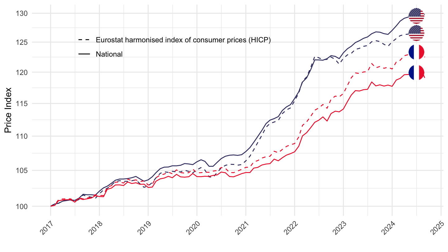
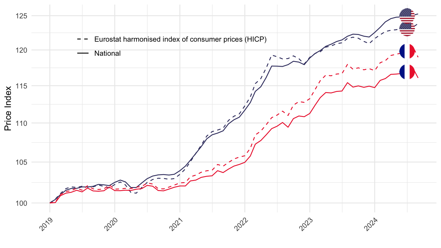
2019-
Code
PRICES_ALL %>%
  filter(EXPENDITURE == "_T",
         REF_AREA %in% c("FRA", "USA"),
         ADJUSTMENT == "N",
         MEASURE == "CPI",
         TRANSFORMATION == "_Z",
         FREQ == "M") %>%


  month_to_date() %>%
  filter(date >= as.Date("2019-01-01")) %>%
  group_by(Ref_area, Methodology) %>%
  arrange(date) %>%
  mutate(obsValue = 100*obsValue/obsValue[1]) %>%
  left_join(colors, by = c("Ref_area"  = "country")) %>%
  ggplot(.) + geom_line(aes(x = date, y = obsValue, color = color, linetype = Methodology)) +
  scale_color_identity() +
  scale_linetype_manual(values = c("dashed", "solid")) + add_flags +
  theme_minimal() + xlab("") + ylab("Price Index") +
  scale_x_date(breaks = seq(1960, 2100, 1) %>% paste0("-01-01") %>% as.Date,
               labels = date_format("%Y")) +
  theme(legend.position = c(0.35, 0.8),
        legend.title = element_blank(),
        axis.text.x = element_text(angle = 45, vjust = 1, hjust = 1)) +
  scale_y_log10(breaks = seq(10, 200, 5))