| source | dataset | Title | .html | .rData |
|---|---|---|---|---|
| eurostat | prc_hicp_manr | HICP (2015 = 100) - monthly data (annual rate of change) | 2026-07-21 | 2026-07-21 |
| eurostat | prc_hicp_aind | HICP (2015 = 100) - annual data (average index and rate of change) | 2026-07-21 | 2026-07-22 |
| eurostat | prc_hicp_cow | HICP - country weights | 2026-07-21 | 2026-07-21 |
| eurostat | nama_10_co3_p3 | Final consumption expenditure of households by consumption purpose (COICOP 3 digit) | 2026-07-18 | 2026-07-21 |
HICP (2015 = 100) - annual data (average index and rate of change)
Data - Eurostat
Info
Data on inflation
| source | dataset | Title | .html | .rData |
|---|---|---|---|---|
| bis | CPI | Consumer Price Index | 2026-07-21 | 2026-07-21 |
| ecb | CES | Consumer Expectations Survey | 2026-07-21 | 2026-07-19 |
| eurostat | nama_10_co3_p3 | Final consumption expenditure of households by consumption purpose (COICOP 3 digit) | 2026-07-18 | 2026-07-21 |
| eurostat | prc_hicp_cow | HICP - country weights | 2026-07-21 | 2026-07-21 |
| eurostat | prc_hicp_ctrb | Contributions to euro area annual inflation (in percentage points) | 2026-07-21 | 2026-07-21 |
| eurostat | prc_hicp_inw | HICP - item weights | 2026-07-21 | 2026-07-21 |
| eurostat | prc_hicp_manr | HICP (2015 = 100) - monthly data (annual rate of change) | 2026-07-21 | 2026-07-21 |
| eurostat | prc_hicp_midx | HICP (2015 = 100) - monthly data (index) | 2026-07-21 | 2026-07-21 |
| eurostat | prc_hicp_mmor | HICP (2015 = 100) - monthly data (monthly rate of change) | 2026-07-21 | 2026-07-21 |
| eurostat | prc_ppp_ind | Purchasing power parities (PPPs), price level indices and real expenditures for ESA 2010 aggregates | 2026-07-21 | 2026-07-21 |
| eurostat | sts_inpp_m | Producer prices in industry, total - monthly data | 2026-07-21 | 2026-07-21 |
| eurostat | sts_inppd_m | Producer prices in industry, domestic market - monthly data | 2026-07-21 | 2026-07-21 |
| eurostat | sts_inppnd_m | Producer prices in industry, non domestic market - monthly data | 2026-07-21 | 2026-07-21 |
| fred | cpi | Consumer Price Index | 2026-07-22 | 2026-07-22 |
| fred | inflation | Inflation | 2026-07-22 | 2026-07-22 |
| imf | CPI | Consumer Price Index (CPI) 2026 February - CPI_2026_FEB_VINTAGE | 2026-07-21 | 2026-04-13 |
| oecd | MEI_PRICES_PPI | Producer Prices - MEI_PRICES_PPI | 2026-07-21 | 2024-04-15 |
| oecd | PPP2017 | 2017 PPP Benchmark results | 2024-04-16 | 2023-07-25 |
| oecd | PRICES_CPI | Consumer price indices (CPIs) | 2024-04-16 | 2024-04-15 |
| wdi | FP.CPI.TOTL.ZG | Inflation, consumer prices (annual %) | 2026-07-21 | 2026-07-21 |
| wdi | NY.GDP.DEFL.KD.ZG | Inflation, GDP deflator (annual %) | 2026-07-21 | 2026-07-21 |
LAST_COMPILE
| LAST_COMPILE |
|---|
| 2026-07-22 |
Last
Code
prc_hicp_aind %>%
  group_by(time) %>%
  summarise(Nobs = n()) %>%
  arrange(desc(time)) %>%
  head(2) %>%
print_table_conditional()| time | Nobs |
|---|---|
| 2025 | 32549 |
| 2024 | 32554 |
unit
Code
prc_hicp_aind %>%
  left_join(unit, by = "unit") %>%
  group_by(unit, Unit) %>%
  summarise(Nobs = n()) %>%
  arrange(-Nobs) %>%
{if (is_html_output()) print_table(.) else .}| unit | Unit | Nobs |
|---|---|---|
| INX_A_AVG | Annual average index | 310631 |
| RCH_A_AVG | Annual average rate of change | 294715 |
| CID_EA | Core inflation differential vis-à-vis the euro area | 696 |
coicop
Code
prc_hicp_aind %>%
  left_join(coicop, by = "coicop") %>%
  group_by(coicop, Coicop) %>%
  summarise(Nobs = n()) %>%
  arrange(-Nobs) %>%
  {if (is_html_output()) datatable(., filter = 'top', rownames = F) else .}
geo
Code
prc_hicp_aind %>%
  left_join(geo, by = "geo") %>%
  group_by(geo, Geo) %>%
  summarise(Nobs = n()) %>%
  arrange(-Nobs) %>%
  mutate(Geo = ifelse(geo == "DE", "Germany", Geo)) %>%
  mutate(Flag = gsub(" ", "-", str_to_lower(Geo)),
         Flag = paste0('<img src="../../bib/flags/vsmall/', Flag, '.png" alt="Flag">')) %>%
  select(Flag, everything()) %>%
  {if (is_html_output()) datatable(., filter = 'top', rownames = F, escape = F) else .}
time
Code
prc_hicp_aind %>%
  group_by(time) %>%
  summarise(Nobs = n()) %>%
  {if (is_html_output()) datatable(., filter = 'top', rownames = F) else .}
Années
2025
Tous
Code
load_data("eurostat/coicop_fr.RData")
prc_hicp_aind %>%
  filter(time == "2025",
         geo %in% c("DE", "FR", "IT", "EA20"),
         unit == "RCH_A_AVG") %>%
  select_if(~ n_distinct(.) > 1) %>%
  left_join(coicop, by = "coicop") %>%
  spread(geo, values) %>%
  select(coicop, Coicop, FR, EA20, everything()) %>%
  {if (is_html_output()) datatable(., filter = 'top', rownames = F) else .}
Sélection
Code
load_data("eurostat/coicop_fr.RData")
prc_hicp_aind %>%
  filter(time == "2025",
         geo %in% c("DE", "FR", "IT", "EA20"),
         unit == "RCH_A_AVG",
         coicop %in% c(paste0("CP0", 0:9), paste0("CP1", 0:3), "CP041", "CP0830")) %>%
  select_if(~ n_distinct(.) > 1) %>%
  left_join(coicop, by = "coicop") %>%
  spread(geo, values) %>%
  select(coicop, Coicop, FR, EA20, everything()) %>%
  View
Quality
Code
compare_coicop <- function(CPname, legend.position = c(0.2, 0.2), start = 1996, geos = c("DE", "FR", "IT", "ES", "NL"), ytick = 10){

  inflation <- prc_hicp_aind %>%
  filter(unit == "INX_A_AVG",
          coicop == CPname,
         geo %in% geos) %>%
  left_join(geo, by = "geo") %>%
  select(geo, Geo, coicop, time, values) %>%
  arrange(time) %>%
  year_to_date %>%
  filter(date >= as.Date(paste0(start, "-01-01"))) %>%
  left_join(colors, by = c("Geo" = "country")) %>%
  group_by(Geo) %>%
  arrange(date) %>%
  mutate(values = 100*values/values[1]) %>%
  ungroup %>%
  mutate(variable = "Price index")

  cons <- nama_10_co3_p3 %>%
  filter(unit == "PD15_EUR",
         geo %in% geos,
         coicop == CPname) %>%
  left_join(geo, by = "geo") %>%
  year_to_date %>%
  filter(date >= as.Date(paste0(start, "-01-01"))) %>%
  left_join(colors, by = c("Geo" = "country")) %>%
  group_by(Geo) %>%
  arrange(date) %>%
  mutate(values = 100*values/values[1]) %>%
  ungroup %>%
  mutate(variable = "Consumption Deflator")

  cons %>%
  bind_rows(inflation) %>%
  ggplot + geom_line(aes(x = date, y = values, color = color, linetype = variable)) +
  theme_minimal()  +
  scale_color_identity() + xlab("") + ylab(CPname) +
  scale_x_date(breaks = as.Date(paste0(seq(1960, 2100, 2), "-01-01")),
               labels = date_format("%Y")) +
  theme(legend.position = legend.position,
        legend.title = element_blank()) +
  scale_y_log10(breaks = seq(10, 1000, ytick))
}


compare_coicop2 <- function(CPname, CPname2, legend.position = c(0.2, 0.2), start = 1996, geos = c("DE", "FR", "IT", "ES", "NL"), ytick = 10){

  inflation <- prc_hicp_aind %>%
  filter(unit == "INX_A_AVG",
          coicop == CPname,
         geo %in% geos) %>%
  left_join(geo, by = "geo") %>%
  select(geo, Geo, coicop, time, values) %>%
  arrange(time) %>%
  year_to_date %>%
  left_join(colors, by = c("Geo" = "country")) %>%
  filter(date >= as.Date(paste0(start, "-01-01"))) %>%
  group_by(Geo) %>%
  arrange(date) %>%
  mutate(values = 100*values/values[1]) %>%
  ungroup %>%
  mutate(variable = "Price index")

  cons <- nama_10_co3_p3 %>%
  filter(unit == "PD15_EUR",
         geo %in% geos,
         coicop == CPname2) %>%
  left_join(geo, by = "geo") %>%
  year_to_date %>%
  filter(date >= as.Date(paste0(start, "-01-01"))) %>%
  left_join(colors, by = c("Geo" = "country")) %>%
  group_by(Geo) %>%
  arrange(date) %>%
  mutate(values = 100*values/values[1]) %>%
  ungroup %>%
  mutate(variable = "Consumption Deflator")

  cons %>%
  bind_rows(inflation) %>%
  ggplot + geom_line(aes(x = date, y = values, color = color, linetype = variable)) +
  theme_minimal()  +
  scale_color_identity() + xlab("") + ylab(CPname) +
  scale_x_date(breaks = as.Date(paste0(seq(1960, 2100, 2), "-01-01")),
               labels = date_format("%Y")) +
  theme(legend.position = legend.position,
        legend.title = element_blank()) +
  scale_y_log10(breaks = seq(10, 1000, ytick))
}
CP00
All
Code
compare_coicop2("CP00", "TOTAL", legend.position = c(0.2, 0.8))
DE, FR
Code
compare_coicop2("CP00", "TOTAL", geos = c("DE", "FR"), legend.position = c(0.2, 0.8))
CP09
Code
prc_hicp_aind %>%
  filter(unit == "INX_A_AVG",
         coicop %in% c("CP09"),
         geo %in% c("DE", "FR", "IT", "ES", "NL")) %>%
  left_join(geo, by = "geo") %>%
  select(geo, Geo, coicop, time, values) %>%
  arrange(time) %>%
  year_to_date %>%
  group_by(Geo) %>%
  arrange(date) %>%
  mutate(values = 100*values/values[1]) %>%
  left_join(colors, by = c("Geo" = "country")) %>%
  ggplot(.) + geom_line(aes(x = date, y = values, color = color)) +
  theme_minimal() + xlab("") + ylab("CP09") +
  scale_x_date(breaks = seq(1960, 2100, 2) %>% paste0("-01-01") %>% as.Date,
               labels = date_format("%Y")) +
  scale_y_log10(breaks = c(seq(0, 200, 10), 2, 3, 5, 15, 8, 4)) +
  scale_color_identity() + add_5flags +
  theme(legend.position = "none")
CP08 - Communications
Annual Inflation
Code
inflation_CP08 <- prc_hicp_aind %>%
  filter(unit == "INX_A_AVG",
         coicop %in% c("CP08"),
         geo %in% c("DE", "FR", "IT", "ES", "NL")) %>%
  left_join(geo, by = "geo") %>%
  select(geo, Geo, coicop, time, values) %>%
  arrange(time) %>%
  year_to_date %>%
  left_join(colors, by = c("Geo" = "country")) %>%
  group_by(Geo) %>%
  arrange(date) %>%
  mutate(values = 100*values/values[1]) %>%
  ungroup %>%
  mutate(variable = "Price index")

inflation_CP08 %>%
  ggplot(.) + geom_line(aes(x = date, y = values, color = color)) +
  theme_minimal() + xlab("") + ylab("CP08") +
  scale_x_date(breaks = seq(1960, 2100, 2) %>% paste0("-01-01") %>% as.Date,
               labels = date_format("%Y")) +
  scale_y_log10(breaks = c(seq(0, 200, 10), 2, 3, 5, 15, 8, 4)) +
  scale_color_identity() + add_5flags +
  theme(legend.position = "none")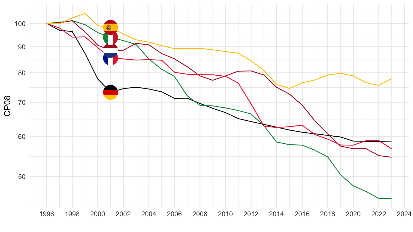
Annual Consumption Deflator Inflation
Code
cons_CP08 <- nama_10_co3_p3 %>%
  filter(unit == "PD15_EUR",
         geo %in% c("FR", "NL", "IT", "DE", "ES"),
         coicop == "CP08") %>%
  left_join(geo, by = "geo") %>%
  year_to_date %>%
  filter(date >= as.Date("1996-01-01")) %>%
  left_join(colors, by = c("Geo" = "country")) %>%
  group_by(Geo) %>%
  arrange(date) %>%
  mutate(values = 100*values/values[1]) %>%
  ungroup %>%
  mutate(variable = "Consumption Deflator")

cons_CP08 %>%
  ggplot + geom_line(aes(x = date, y = values, color = color)) +
  theme_minimal()  + add_5flags +
  scale_color_identity() + xlab("") + ylab("Communications (08)") +
  scale_x_date(breaks = as.Date(paste0(seq(1960, 2100, 2), "-01-01")),
               labels = date_format("%Y")) +
  theme(legend.position = c(0.2, 0.85),
        legend.title = element_blank()) +
  scale_y_log10(breaks = seq(10, 300, 10))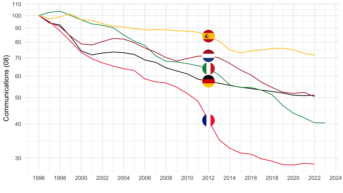
Bind
Code
compare_coicop("CP08")
CP081 - Postal services
Bind
Code
compare_coicop("CP081", legend.position = c(0.2, 0.8))
CP082_083
CP0820
Bind
Code
compare_coicop2("CP0820", "CP082", legend.position = c(0.2, 0.8))
CP0830
Bind
Code
compare_coicop2("CP0830", "CP083", legend.position = c(0.2, 0.2))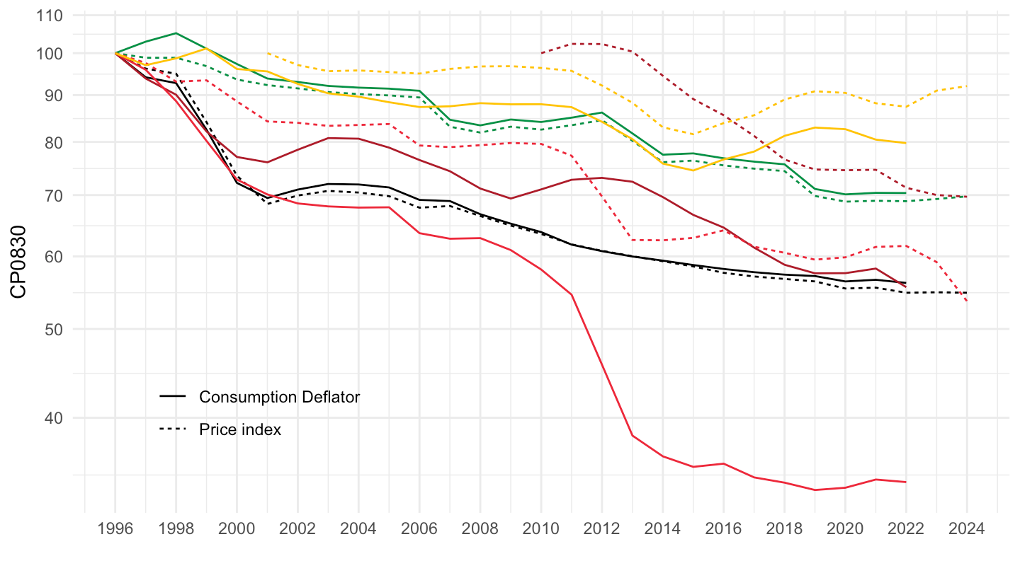
Annual Consumption Deflator Inflation
Code
cons_CP083 <- nama_10_co3_p3 %>%
  filter(unit == "PD15_EUR",
         geo %in% c("FR", "NL", "IT", "DE", "ES"),
         coicop == "CP083") %>%
  left_join(geo, by = "geo") %>%
  year_to_date %>%
  filter(date >= as.Date("1996-01-01")) %>%
  left_join(colors, by = c("Geo" = "country")) %>%
  group_by(Geo) %>%
  arrange(date) %>%
  mutate(values = 100*values/values[1]) %>%
  ungroup %>%
  mutate(variable = "Consumption Deflator")

cons_CP083 %>%
  ggplot + geom_line(aes(x = date, y = values, color = color)) +
  theme_minimal()  + add_5flags +
  scale_color_identity() + xlab("") + ylab("Communications (083)") +
  scale_x_date(breaks = as.Date(paste0(seq(1960, 2100, 2), "-01-01")),
               labels = date_format("%Y")) +
  theme(legend.position = c(0.2, 0.85),
        legend.title = element_blank()) +
  scale_y_log10(breaks = seq(10, 300, 10))
CP071
Bind
Code
compare_coicop("CP071", legend.position = c(0.2, 0.8))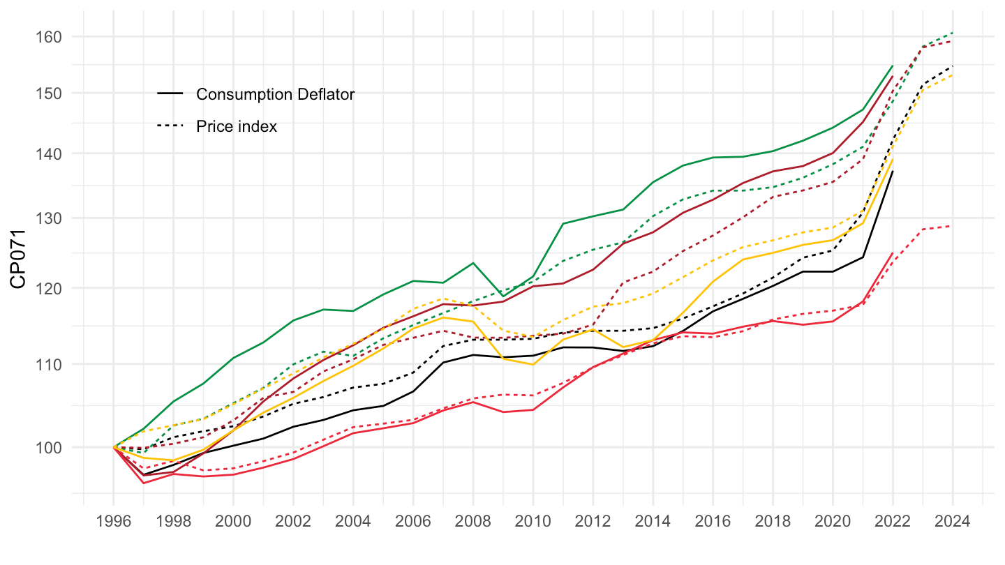
CP041
Bind
Code
compare_coicop("CP041", legend.position = c(0.2, 0.8))
1999-
Code
compare_coicop("CP041", legend.position = c(0.2, 0.8), start = 1999)
2000-
Code
compare_coicop("CP041", legend.position = c(0.2, 0.8), start = 2000)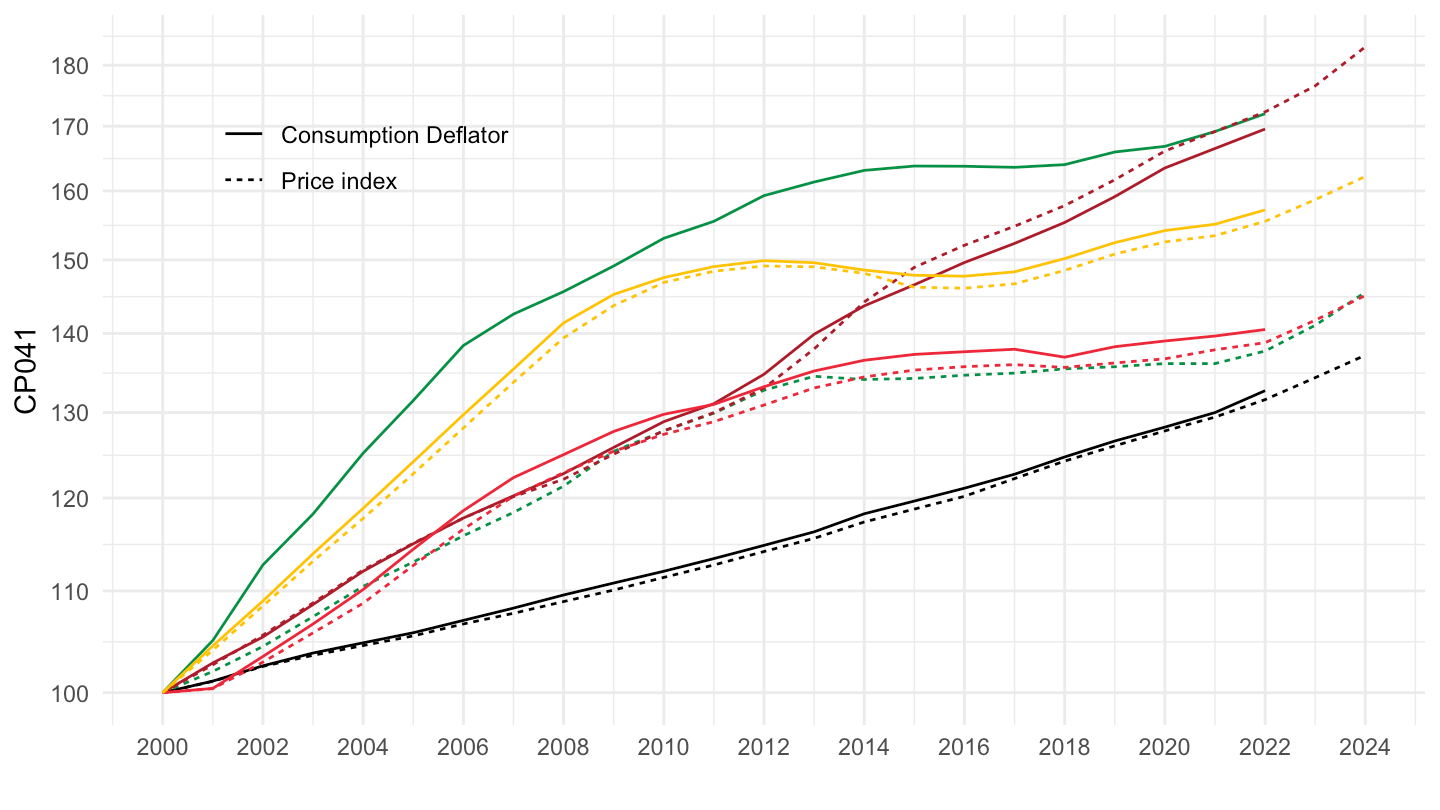
CP01
Bind
Code
compare_coicop("CP01", legend.position = c(0.2, 0.8))
CP02
Bind
Code
compare_coicop("CP02", legend.position = c(0.2, 0.8))
CP022
Bind
Code
compare_coicop("CP022", legend.position = c(0.2, 0.8), ytick = 50)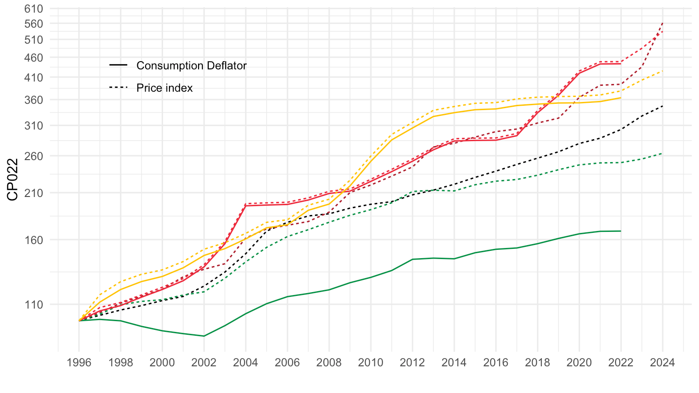
CP03
Bind
Code
compare_coicop("CP03", legend.position = c(0.2, 0.8))
CP04
Bind
Code
compare_coicop("CP04", legend.position = c(0.2, 0.8))
CP05
Bind
Code
compare_coicop("CP05", legend.position = c(0.2, 0.8))
CP06
Bind
Code
compare_coicop("CP06", legend.position = c(0.2, 0.8))
CP07
Bind
Code
compare_coicop("CP07", legend.position = c(0.2, 0.8))
CP09
Bind
Code
compare_coicop("CP09")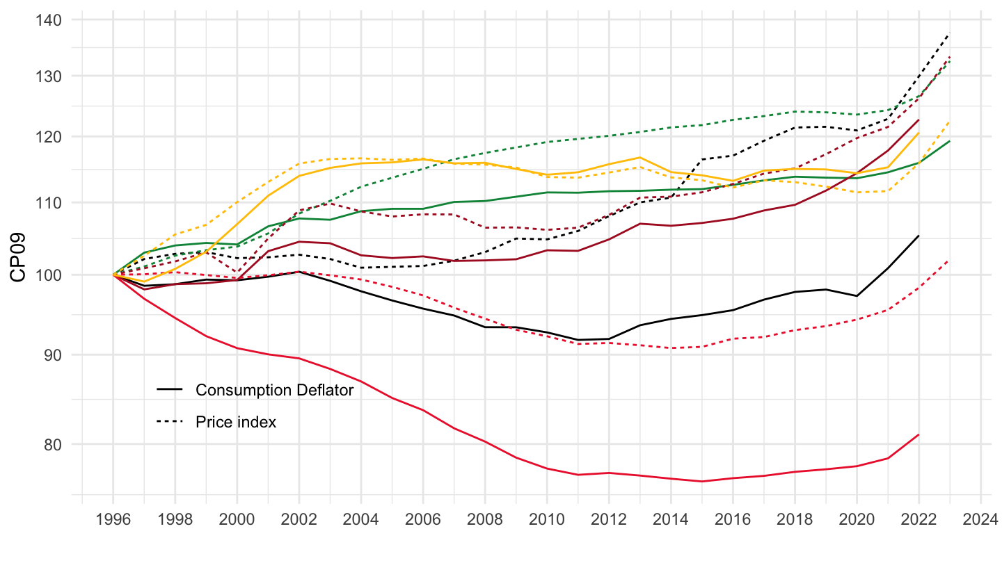
CP091
Bind
Code
compare_coicop("CP091")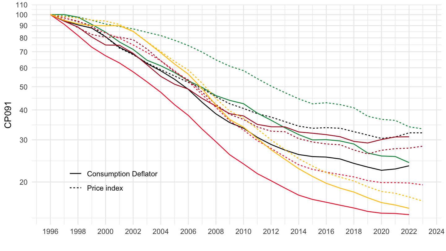
CP10
Bind
Code
compare_coicop("CP10", legend.position = c(0.2, 0.8))
CP11
Bind
Code
compare_coicop("CP11", legend.position = c(0.2, 0.8))
CP12
Bind
Code
compare_coicop("CP12", legend.position = c(0.2, 0.8))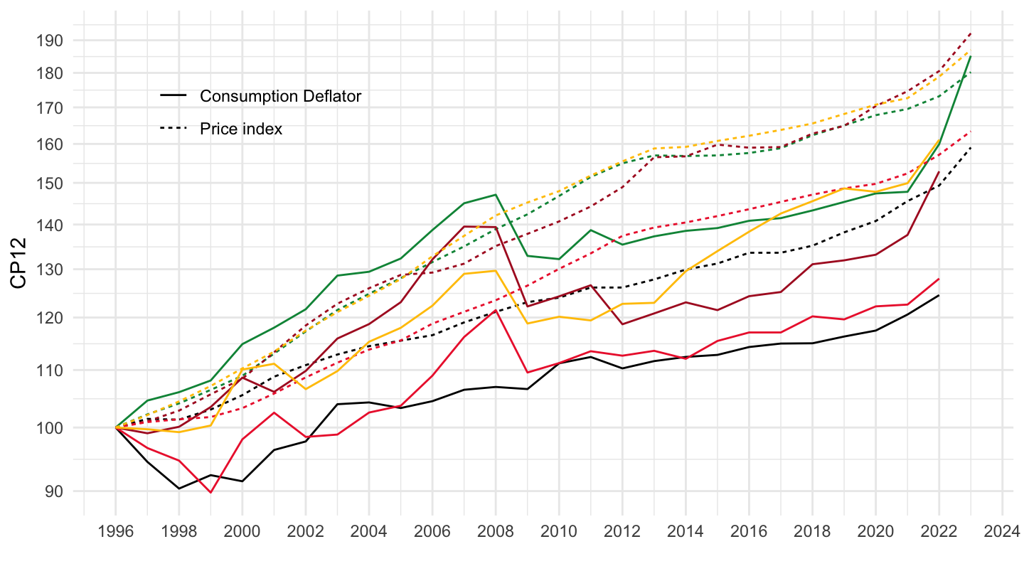
CP082_083 - Telephone and telefax equipment
Code
prc_hicp_aind %>%
  filter(unit == "INX_A_AVG",
         coicop %in% c("CP082_083"),
         geo %in% c("DE", "FR", "IT", "ES", "NL")) %>%
  left_join(geo, by = "geo") %>%
  select(geo, Geo, coicop, time, values) %>%
  arrange(time) %>%
  year_to_date %>%
  group_by(Geo) %>%
  arrange(date) %>%
  mutate(values = 100*values/values[1]) %>%
  left_join(colors, by = c("Geo" = "country")) %>%
  ggplot(.) + geom_line(aes(x = date, y = values, color = color)) +
  theme_minimal() + xlab("") + ylab("CP082_083") +
  scale_x_date(breaks = seq(1960, 2100, 2) %>% paste0("-01-01") %>% as.Date,
               labels = date_format("%Y")) +
  scale_y_log10(breaks = c(seq(0, 200, 10), 2, 3, 5, 15, 8, 4)) +
  scale_color_identity() + add_5flags +
  theme(legend.position = "none")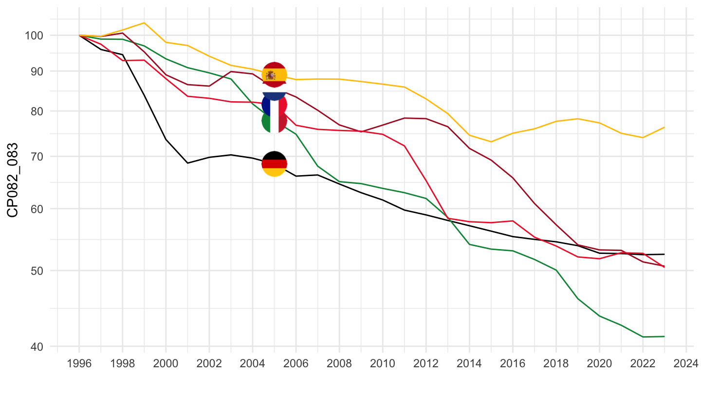
CP0820 - Telephone and telefax equipment
Code
prc_hicp_aind %>%
  filter(unit == "INX_A_AVG",
         coicop %in% c("CP0820"),
         geo %in% c("DE", "FR", "IT", "ES", "NL")) %>%
  left_join(geo, by = "geo") %>%
  select(geo, Geo, coicop, time, values) %>%
  arrange(time) %>%
  year_to_date %>%
  group_by(Geo) %>%
  arrange(date) %>%
  mutate(values = 100*values/values[1]) %>%
  left_join(colors, by = c("Geo" = "country")) %>%
  ggplot(.) + geom_line(aes(x = date, y = values, color = color)) +
  theme_minimal() + xlab("") + ylab("CP0820 - Telephone and telefax equipment") +
  scale_x_date(breaks = seq(1960, 2100, 2) %>% paste0("-01-01") %>% as.Date,
               labels = date_format("%Y")) +
  scale_y_log10(breaks = c(seq(0, 200, 10), 2, 3, 5, 15, 8, 4)) +
  scale_color_identity() + add_3flags +
  theme(legend.position = "none")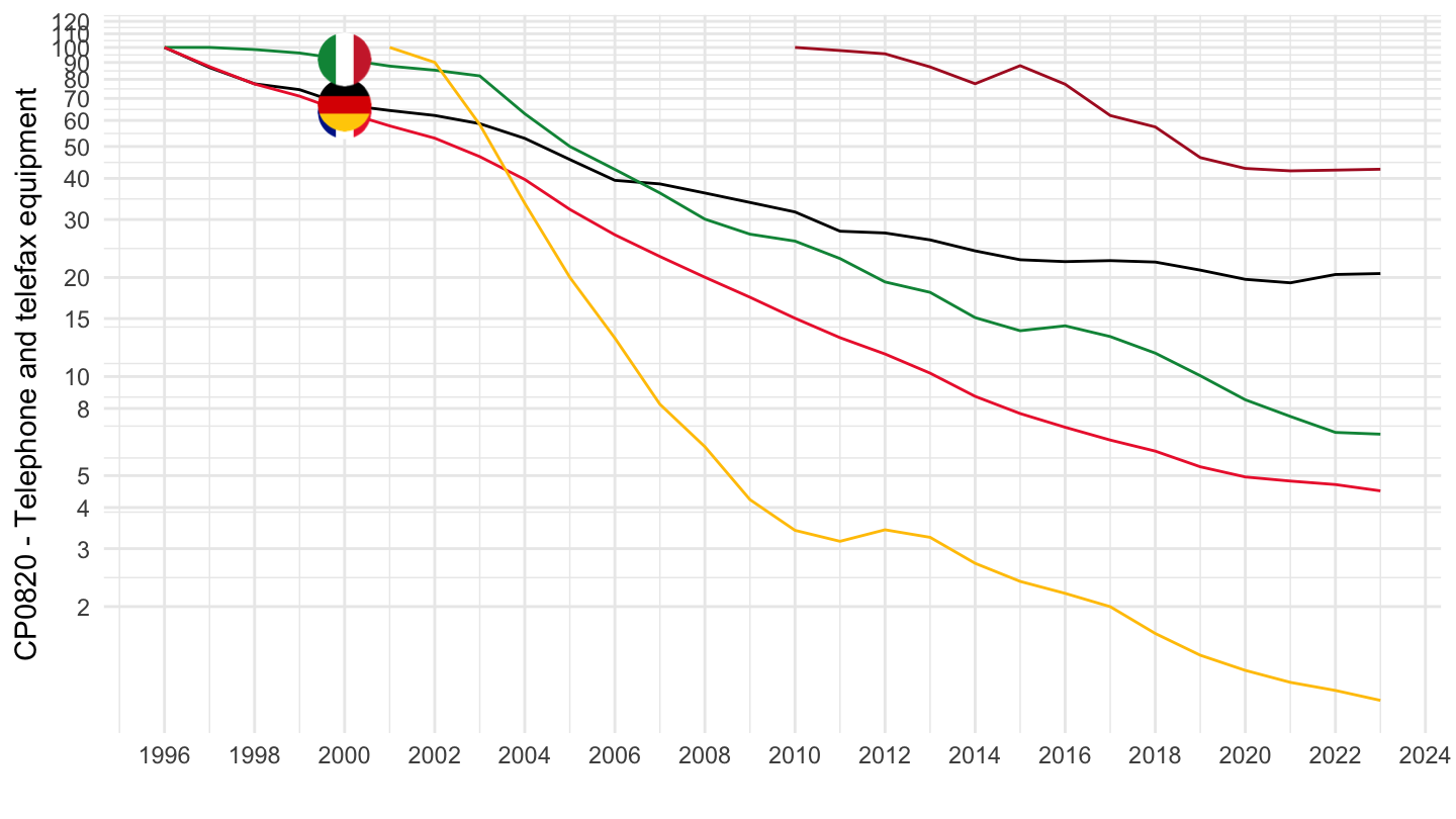
Code
prc_hicp_aind %>%
  filter(unit == "INX_A_AVG",
         coicop %in% c("CP082_083"),
         geo %in% c("DE", "FR", "IT", "ES", "NL")) %>%
  left_join(geo, by = "geo") %>%
  select(geo, Geo, coicop, time, values) %>%
  arrange(time) %>%
  year_to_date %>%
  group_by(Geo) %>%
  arrange(date) %>%
  mutate(values = 100*values/values[1]) %>%
  left_join(colors, by = c("Geo" = "country")) %>%
  ggplot(.) + geom_line(aes(x = date, y = values, color = color)) +
  theme_minimal() + xlab("") + ylab("CP082_083") +
  scale_x_date(breaks = seq(1960, 2100, 2) %>% paste0("-01-01") %>% as.Date,
               labels = date_format("%Y")) +
  scale_y_log10(breaks = c(seq(0, 200, 10), 2, 3, 5, 15, 8, 4)) +
  scale_color_identity() + add_5flags +
  theme(legend.position = "none")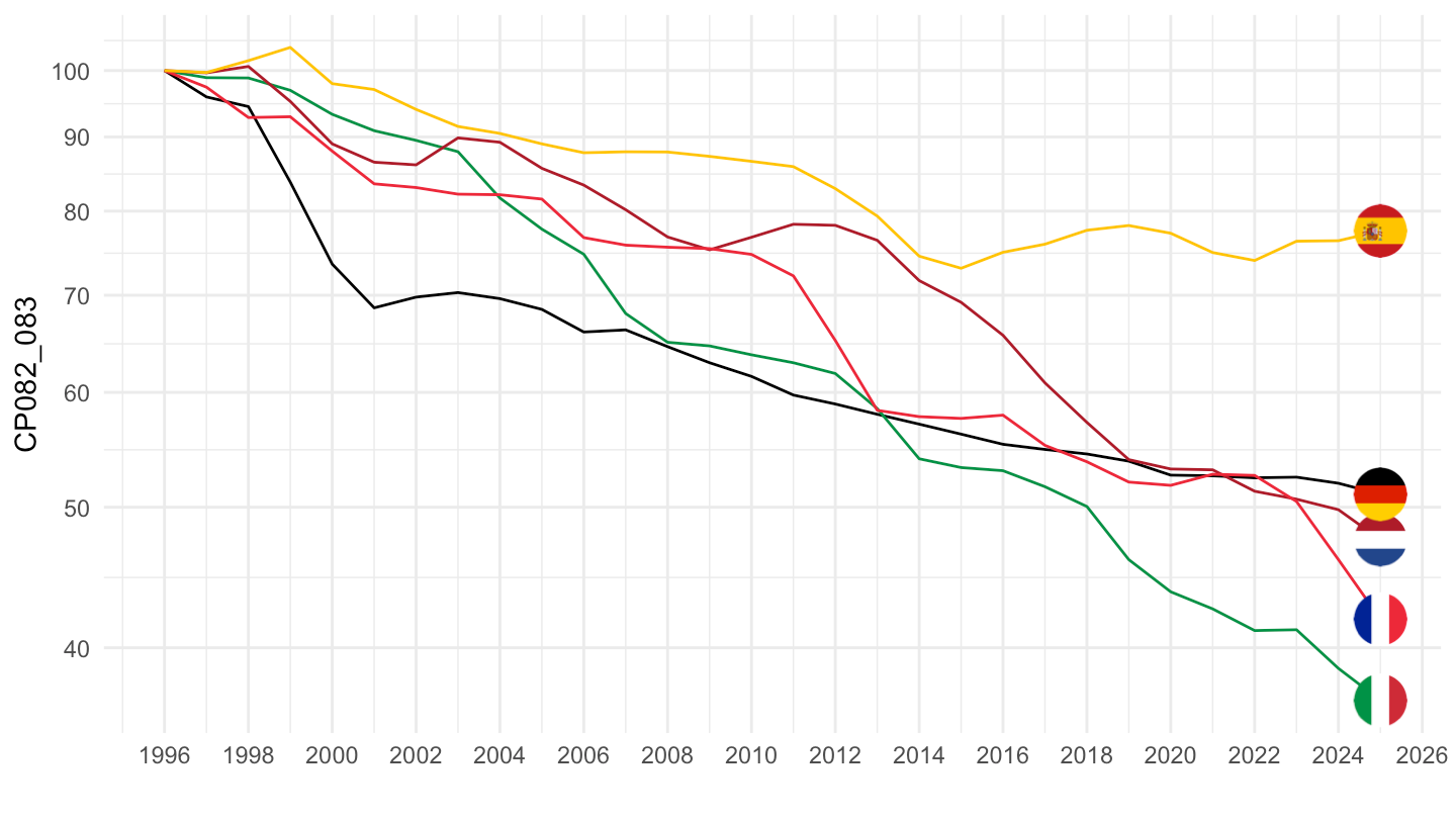
CP091
Code
prc_hicp_aind %>%
  filter(unit == "INX_A_AVG",
         coicop %in% c("CP091"),
         geo %in% c("DE", "FR", "IT", "ES", "NL")) %>%
  left_join(geo, by = "geo") %>%
  select(geo, Geo, coicop, time, values) %>%
  arrange(time) %>%
  year_to_date %>%
  group_by(Geo) %>%
  arrange(date) %>%
  mutate(values = 100*values/values[1]) %>%
  left_join(colors, by = c("Geo" = "country")) %>%
  ggplot(.) + geom_line(aes(x = date, y = values, color = color)) +
  theme_minimal() + xlab("") + ylab("CP091") +
  scale_x_date(breaks = seq(1960, 2100, 2) %>% paste0("-01-01") %>% as.Date,
               labels = date_format("%Y")) +
  scale_y_log10(breaks = c(seq(0, 200, 10), 2, 3, 5, 15, 8, 4)) +
  scale_color_identity() + add_5flags +
  theme(legend.position = "none")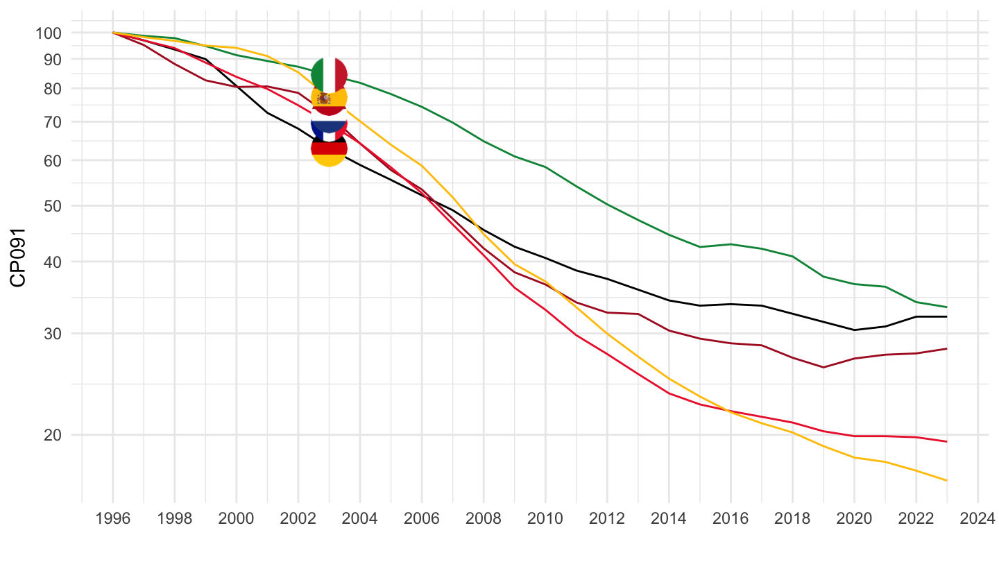
CP071 - Cars
Code
prc_hicp_aind %>%
  filter(unit == "INX_A_AVG",
         coicop %in% c("CP071"),
         geo %in% c("DE", "FR", "IT", "ES", "NL")) %>%
  left_join(geo, by = "geo") %>%
  select(geo, Geo, coicop, time, values) %>%
  arrange(time) %>%
  year_to_date %>%
  group_by(Geo) %>%
  arrange(date) %>%
  mutate(values = 100*values/values[1]) %>%
  left_join(colors, by = c("Geo" = "country")) %>%
  ggplot(.) + geom_line(aes(x = date, y = values, color = color)) +
  theme_minimal() + xlab("") + ylab("CP071 - Cars") +
  scale_x_date(breaks = seq(1960, 2100, 2) %>% paste0("-01-01") %>% as.Date,
               labels = date_format("%Y")) +
  scale_y_log10(breaks = c(seq(0, 200, 10), 2, 3, 5, 15, 8, 4)) +
  scale_color_identity() + add_5flags +
  theme(legend.position = "none")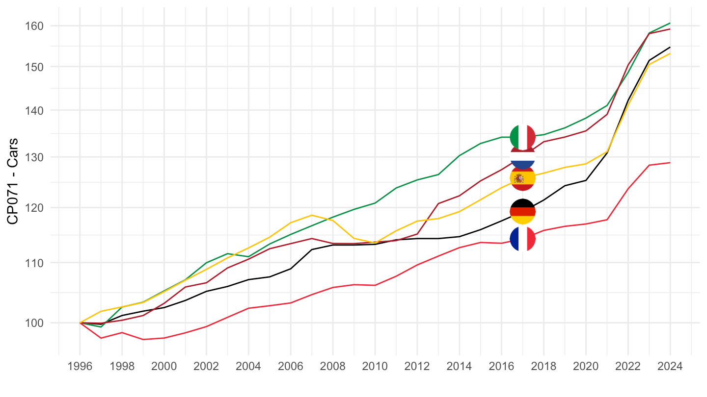
CP03 - Clothing
2017-
Code
prc_hicp_aind %>%
  filter(unit == "INX_A_AVG",
         coicop %in% c("CP03"),
         geo %in% c("DE", "FR", "IT", "ES", "EA20")) %>%
  left_join(geo, by = "geo") %>%
  select(geo, Geo, coicop, time, values) %>%
  arrange(time) %>%
  year_to_date %>%
  group_by(Geo) %>%
  arrange(date) %>%
  filter(date >= as.Date("2017-01-01")) %>%
  mutate(values = 100*values/values[1]) %>%
  left_join(colors, by = c("Geo" = "country")) %>%
  ggplot(.) + geom_line(aes(x = date, y = values, color = color)) +
  theme_minimal() + xlab("") + ylab("CP03 - Clothing and footwear") +
  scale_x_date(breaks = seq(1960, 2100, 1) %>% paste0("-01-01") %>% as.Date,
               labels = date_format("%Y")) +
  scale_y_log10(breaks = c(seq(0, 200, 1), 2, 3, 5, 15, 8, 4)) +
  scale_color_identity() + add_5flags +
  theme(legend.position = "none")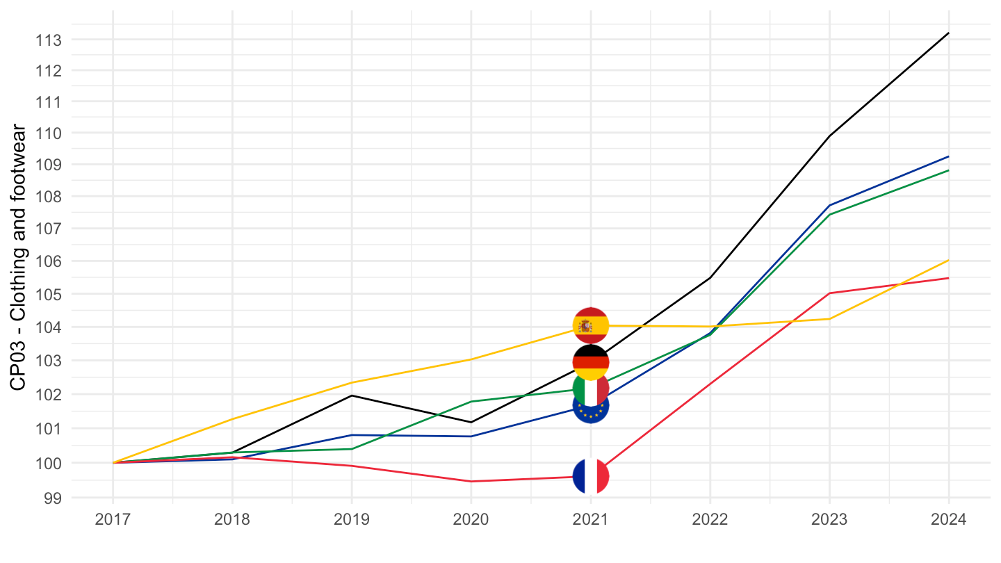
CP08202 - Mobile Telephone equipment
2017-
Code
prc_hicp_aind %>%
  filter(unit == "INX_A_AVG",
         coicop %in% c("CP08202"),
         geo %in% c("DE", "FR", "IT", "ES", "EA20")) %>%
  left_join(geo, by = "geo") %>%
  select(geo, Geo, coicop, time, values) %>%
  arrange(time) %>%
  year_to_date %>%
  group_by(Geo) %>%
  arrange(date) %>%
  filter(date >= as.Date("2017-01-01")) %>%
  mutate(values = 100*values/values[1]) %>%
  left_join(colors, by = c("Geo" = "country")) %>%
  ggplot(.) + geom_line(aes(x = date, y = values, color = color)) +
  theme_minimal() + xlab("") + ylab("CP08202 - Mobile Telephone equipment") +
  scale_x_date(breaks = seq(1960, 2100, 1) %>% paste0("-01-01") %>% as.Date,
               labels = date_format("%Y")) +
  scale_y_log10(breaks = c(seq(0, 200, 10), 2, 3, 5, 15, 8, 4)) +
  scale_color_identity() + add_5flags +
  theme(legend.position = "none")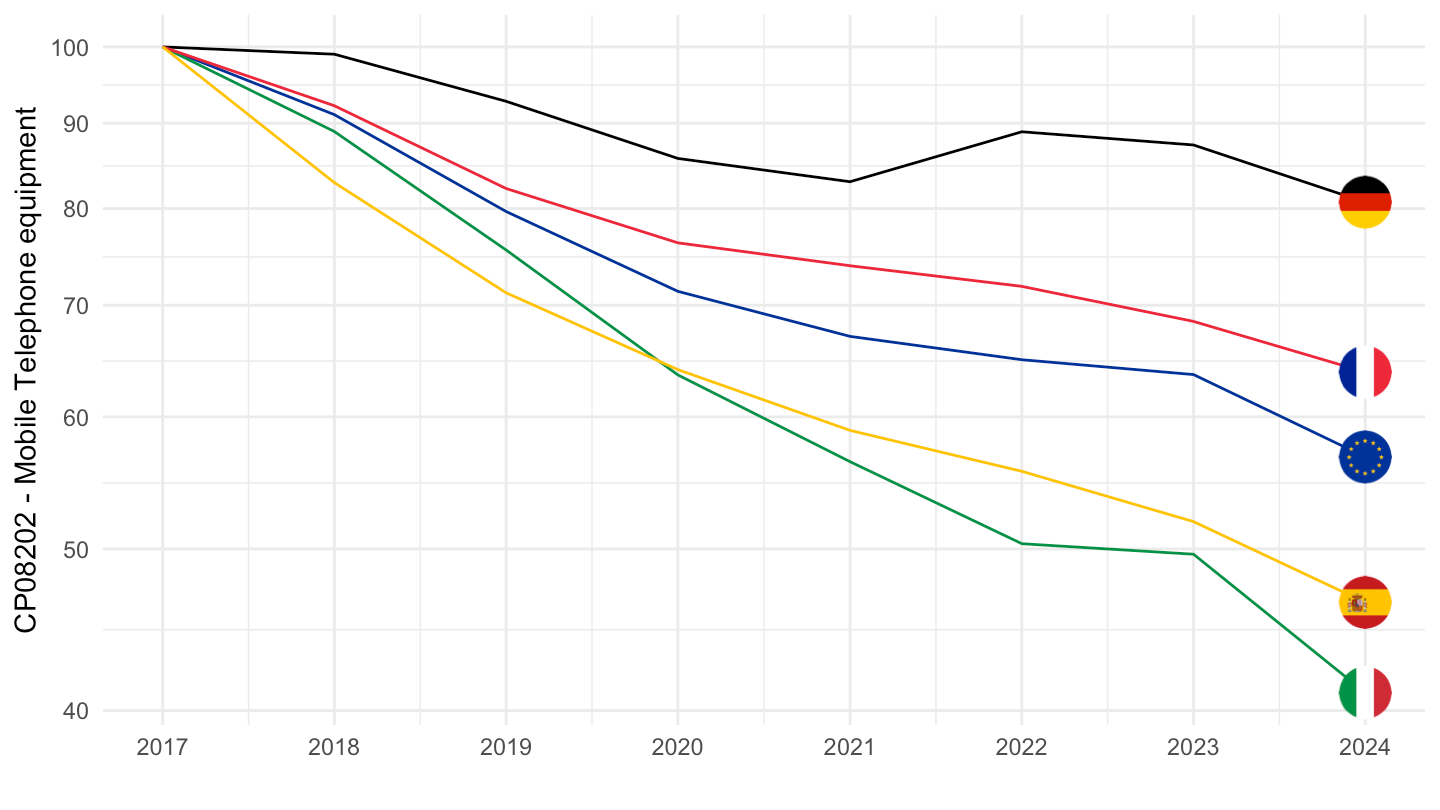
Greece, Europe, France, Spain, Italy, Germany
2011-2013 -
HICP
Code
prc_hicp_aind %>%
  filter(unit == "INX_A_AVG",
         coicop == "CP00",
         geo %in% c("EL", "FR", "ES", "IT", "DE")) %>%
  year_to_date %>%
  group_by(geo) %>%
  mutate(values = 100*values/values[date == as.Date("2011-01-01")]) %>%
  filter(date >= as.Date("2009-01-01"),
         date <= as.Date("2016-01-01")) %>%
  left_join(geo, by = "geo") %>%
  mutate(Geo = ifelse(geo == "EA", "Europe", Geo),
         Geo = ifelse(geo == "DE", "Germany", Geo)) %>%
  left_join(colors, by = c("Geo" = "country")) %>%
  ggplot(.) + geom_line(aes(x = date, y = values, color = color)) +
  theme_minimal() + xlab("") + ylab("100 = Janv. 2011") +
  scale_x_date(breaks = seq(1960, 2021, 1) %>% paste0("-01-01") %>% as.Date,
               labels = date_format("%Y")) +
  scale_color_identity() + add_5flags +
  scale_y_log10(breaks = seq(0, 200, 2)) +
  theme(legend.position = "none",
        legend.title = element_blank())
Rents
Code
prc_hicp_aind %>%
  filter(unit == "INX_A_AVG",
         coicop == "CP041",
         geo %in% c("EL", "FR", "ES", "IT", "DE")) %>%
  year_to_date %>%
  group_by(geo) %>%
  mutate(values = 100*values/values[date == as.Date("2011-01-01")]) %>%
  filter(date >= as.Date("2009-01-01"),
         date <= as.Date("2016-01-01")) %>%
  left_join(geo, by = "geo") %>%
  mutate(Geo = ifelse(geo == "EA", "Europe", Geo),
         Geo = ifelse(geo == "DE", "Germany", Geo)) %>%
  left_join(colors, by = c("Geo" = "country")) %>%
  ggplot(.) + geom_line(aes(x = date, y = values, color = color)) +
  theme_minimal() + xlab("") + ylab("100 = Janv. 2011") +
  scale_x_date(breaks = seq(1960, 2021, 1) %>% paste0("-01-01") %>% as.Date,
               labels = date_format("%Y")) +
  scale_color_identity() + add_5flags +
  scale_y_log10(breaks = seq(0, 200, 2)) +
  theme(legend.position = "none",
        legend.title = element_blank())
Real Rents
Code
prc_hicp_aind %>%
  filter(unit == "INX_A_AVG",
         coicop %in% c("CP041", "CP00"),
         geo %in% c("EL", "FR", "ES", "IT", "DE")) %>%
  left_join(geo, by = "geo") %>%
  select(geo, Geo, coicop, time, values) %>%
  spread(coicop, values) %>%
  mutate(values = 100*CP041/CP00) %>%
  year_to_date %>%
  group_by(geo) %>%
  mutate(values = 100*values/values[date == as.Date("2011-01-01")]) %>%
  filter(date >= as.Date("2009-01-01"),
         date <= as.Date("2016-01-01")) %>%
  mutate(Geo = ifelse(geo == "EA", "Europe", Geo),
         Geo = ifelse(geo == "DE", "Germany", Geo)) %>%
  left_join(colors, by = c("Geo" = "country")) %>%
  ggplot(.) + geom_line(aes(x = date, y = values, color = color)) +
  theme_minimal() + xlab("") + ylab("Real Rents (100 = Janv. 2011)") +
  scale_x_date(breaks = seq(1960, 2021, 1) %>% paste0("-01-01") %>% as.Date,
               labels = date_format("%Y")) +
  scale_color_identity() + add_5flags +
  scale_y_log10(breaks = seq(0, 200, 2)) +
  theme(legend.position = "none",
        legend.title = element_blank())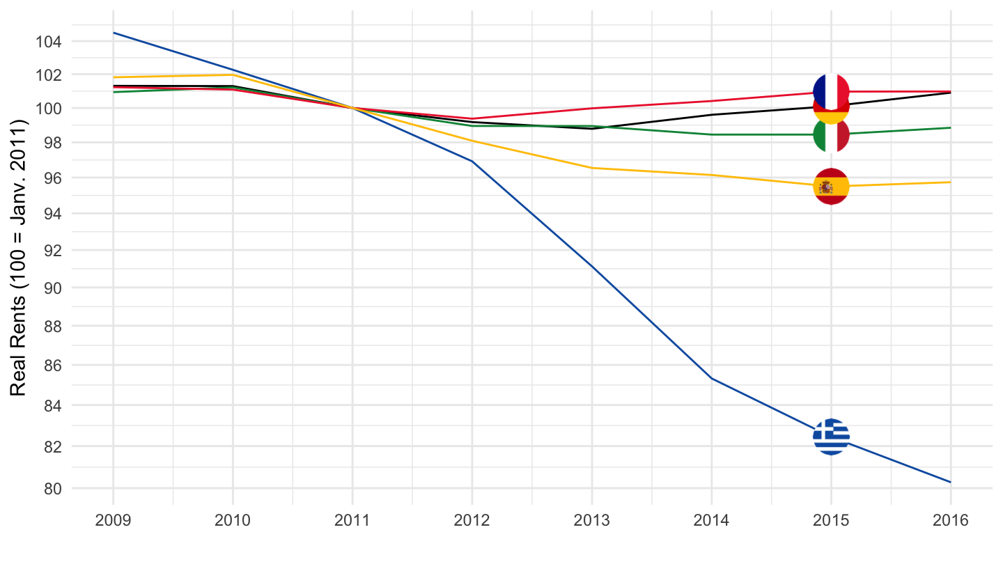
Europe - Real Rents
Value
Code
prc_hicp_aind %>%
  filter(unit == "INX_A_AVG",
         coicop %in% c("CP041", "CP00"),
         geo %in% c("EA")) %>%
  left_join(tibble(geo = c("EA", "EA18", "EA19"),
                   Geo = c("Euro Area (time-dep geography)")),
            by = "geo") %>%
  select(geo, Geo, coicop, time, values) %>%
  spread(coicop, values) %>%
  mutate(values = 100*CP041/CP00) %>%
  year_to_date %>%
  ggplot(.) + geom_line(aes(x = date, y = values)) +
  theme_minimal() + xlab("") + ylab("") +
  scale_x_date(breaks = seq(1960, 2100, 5) %>% paste0("-01-01") %>% as.Date,
               labels = date_format("%Y")) +
  scale_y_log10(breaks = seq(0, 200, 1)) +
  scale_color_manual(values = viridis(5)[1:4]) +
  theme(legend.position = c(0.5, 0.85),
        legend.title = element_blank())