Error in readChar(con, 5L, useBytes = TRUE) :
impossible d'ouvrir la connexionFinancial market data
Data - ECB
Info
LAST_COMPILE
| LAST_COMPILE |
|---|
| 2026-07-24 |
Last
| TIME_PERIOD | FREQ | Nobs |
|---|---|---|
| 2026-Q2 | Q | 23 |
| 2026-07-23 | D | 6 |
| 2026-06-17 | B | 6 |
| 2026-06 | M | 34 |
| 2025 | A | 24 |
Last Day
| TITLE | TIME_PERIOD | OBS_VALUE |
|---|---|---|
| Deposit facility - date of changes (raw data) - Change in percentage points compared to previous rate | 2026-07-23 | 0.25 |
| Deposit facility - date of changes (raw data) - Level | 2026-07-23 | 2.25 |
| Marginal lending facility - date of changes (raw data) - Change in percentage points compared to previous rate | 2026-07-23 | 0.25 |
| Marginal lending facility - date of changes (raw data) - Level | 2026-07-23 | 2.65 |
| Main refinancing operations - fixed rate tenders (fixed rate) (date of changes) - Level | 2026-07-23 | 2.40 |
| Main refinancing operations - Minimum bid rate/fixed rate (date of changes) - Level | 2026-07-23 | 2.40 |
PROVIDER_FM_ID
Code
FM %>%
  left_join(PROVIDER_FM_ID,  by = "PROVIDER_FM_ID") %>%
  group_by(PROVIDER_FM_ID, PROVIDER_FM_ID_desc) %>%
  summarise(Nobs = n()) %>%
  arrange(-Nobs) %>%
  {if (is_html_output()) datatable(., filter = 'top', rownames = F) else .}
FREQ
Code
FM %>%
  left_join(FREQ,  by = "FREQ") %>%
  group_by(FREQ, Freq) %>%
  summarise(Nobs = n()) %>%
{if (is_html_output()) print_table(.) else .}| FREQ | Freq | Nobs |
|---|---|---|
| A | Annual | 930 |
| B | Daily - businessweek | 6312 |
| D | Daily | 60392 |
| M | Monthly | 21737 |
| Q | Quarterly | 3788 |
REF_AREA
Code
FM %>%
  left_join(REF_AREA,  by = "REF_AREA") %>%
  group_by(REF_AREA, Ref_area) %>%
  summarise(Nobs = n()) %>%
  mutate(Flag = gsub(" ", "-", str_to_lower(gsub(" ", "-", Ref_area))),
         Flag = paste0('<img src="../../icon/flag/vsmall/', Flag, '.png" alt="Flag">')) %>%
  select(Flag, everything()) %>%
  {if (is_html_output()) datatable(., filter = 'top', rownames = F, escape = F) else .}
CURRENCY
Code
FM %>%
  left_join(CURRENCY,  by = "CURRENCY") %>%
  group_by(CURRENCY, Currency) %>%
  summarise(Nobs = n()) %>%
  arrange(-Nobs) %>%
{if (is_html_output()) print_table(.) else .}| CURRENCY | Currency | Nobs |
|---|---|---|
| EUR | Euro | 75590 |
| GBP | UK pound sterling | 6742 |
| USD | US dollar | 6320 |
| JPY | Japanese yen | 3636 |
| DKK | Danish krone | 452 |
| SEK | Swedish krona | 419 |
PROVIDER_FM
Code
FM %>%
  left_join(PROVIDER_FM,  by = "PROVIDER_FM") %>%
  group_by(PROVIDER_FM, Provider_fm) %>%
  summarise(Nobs = n()) %>%
  arrange(-Nobs) %>%
{if (is_html_output()) print_table(.) else .}| PROVIDER_FM | Provider_fm | Nobs |
|---|---|---|
| 4F | ECB | 77079 |
| DS | DataStream | 10039 |
| RT | Reuters | 6041 |
INSTRUMENT_FM
Code
FM %>%
  left_join(INSTRUMENT_FM,  by = "INSTRUMENT_FM") %>%
  group_by(INSTRUMENT_FM, Instrument_fm) %>%
  summarise(Nobs = n()) %>%
  arrange(-Nobs) %>%
{if (is_html_output()) print_table(.) else .}| INSTRUMENT_FM | Instrument_fm | Nobs |
|---|---|---|
| KR | Key interest rate | 60987 |
| MM | Money Market | 12193 |
| EI | Equity/index | 9168 |
| BB | Benchmark bond | 7956 |
| CY | Commodity | 1136 |
| BZ | Zero-coupon yield bond | 890 |
| SP | Spread | 829 |
DATA_TYPE_FM
Code
FM %>%
  left_join(DATA_TYPE_FM,  by = "DATA_TYPE_FM") %>%
  group_by(DATA_TYPE_FM, Data_type_fm) %>%
  summarise(Nobs = n()) %>%
  arrange(-Nobs) %>%
{if (is_html_output()) print_table(.) else .}| DATA_TYPE_FM | Data_type_fm | Nobs |
|---|---|---|
| LEV | Level | 40468 |
| CHG | Change in percentage points compared to previous rate | 20316 |
| HSTA | Historical close, average of observations through period | 15909 |
| SPR | Spread | 5920 |
| YLDA | Yield, average of observations through period | 4566 |
| YLD | Yield | 3390 |
| YLDE | Yield, end of period | 890 |
| ASKA | Ask price or primary activity, average of observations through period | 871 |
| SPRE | Spread, end of period | 829 |
COLLECTION
Code
FM %>%
  left_join(COLLECTION,  by = "COLLECTION") %>%
  group_by(COLLECTION, Collection) %>%
  summarise(Nobs = n()) %>%
{if (is_html_output()) print_table(.) else .}| COLLECTION | Collection | Nobs |
|---|---|---|
| A | Average of observations through period | 21367 |
| E | End of period | 71792 |
UNIT
Code
FM %>%
  left_join(UNIT,  by = "UNIT") %>%
  group_by(UNIT, Unit) %>%
  summarise(Nobs = n()) %>%
{if (is_html_output()) print_table(.) else .}| UNIT | Unit | Nobs |
|---|---|---|
| PC | Percent | 20316 |
| PCPA | Percent per annum | 63510 |
| POINTS | Points | 9168 |
| USD | US dollar | 165 |
TITLE
Code
FM %>%
  group_by(TITLE) %>%
  summarise(Nobs = n()) %>%
  {if (is_html_output()) datatable(., filter = 'top', rownames = F) else .}
Real Rates
USA, Euro Area
1999
Code
plot <- FM %>%
  filter(PROVIDER_FM_ID %in% c("R_US10YT_RR", "R_U2_10Y")) %>%
  month_to_date %>%
  left_join(REF_AREA, by = "REF_AREA") %>%
  mutate(Ref_area = ifelse(REF_AREA == "U2", "Zone euro", "États-Unis")) %>%
  filter(date >= as.Date("1999-01-01")) %>%
  mutate(OBS_VALUE = OBS_VALUE/100) %>%
  ggplot(.) + theme_minimal() + xlab("") + ylab("Taux d'intérêt réels à 10 ans") +
  geom_line(aes(x = date, y = OBS_VALUE, color = Ref_area)) +
  scale_color_manual(values = c("#B22234", "#003399")) +
  geom_rect(data = nber_recessions %>%
              filter(Peak > as.Date("1999-01-01")),
            aes(xmin = Peak, xmax = Trough, ymin =-Inf, ymax = +Inf),
            fill = '#B22234', alpha = 0.1)  +
  geom_rect(data = cepr_recessions %>%
              filter(Peak > as.Date("1999-01-01")),
            aes(xmin = Peak, xmax = Trough, ymin = -Inf, ymax = +Inf),
            fill = '#003399', alpha = 0.1)  +
  scale_x_date(breaks = c(seq(1999, 2100, 5), seq(1997, 2100, 5)) %>% paste0("-01-01") %>% as.Date,
               labels = date_format("%Y")) +
  theme(legend.position = c(0.26, 0.2),
        legend.title = element_blank()) +
  scale_y_continuous(breaks = 0.01*seq(-10, 50, 1),
                     labels = percent_format(accuracy = 1)) +
  labs(caption = "Source: BCE, Données sur les marchés financiers")
save(plot, file = "FM_files/figure-html/real-rates-USA-EUR-1999-1.RData")
plot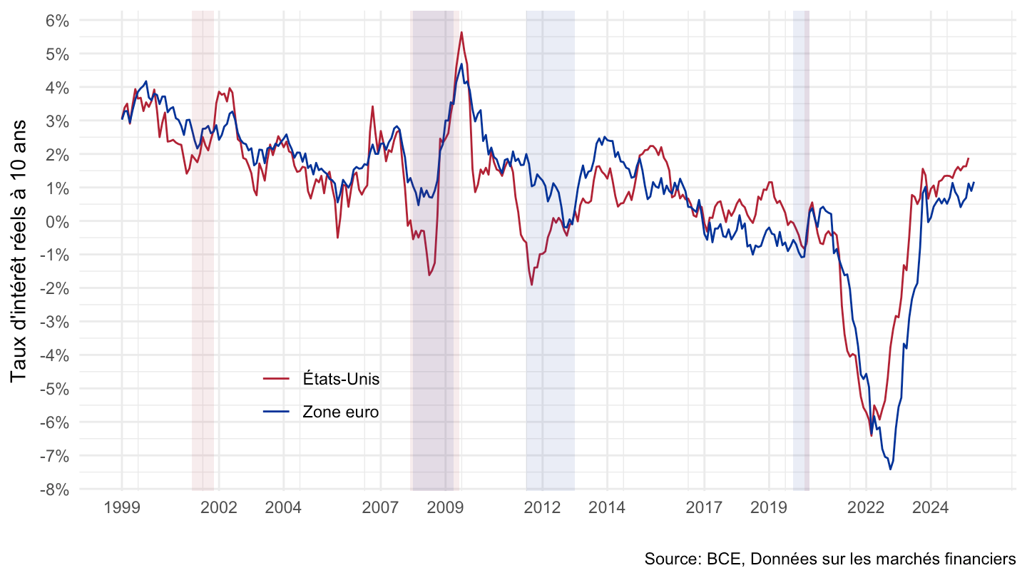
USA, Japan, Euro Area
All
Code
FM %>%
  filter(PROVIDER_FM_ID %in% c("R_US10YT_RR", "R_JP10YT_RR", "R_U2_10Y")) %>%
  month_to_date %>%
  left_join(REF_AREA, by = "REF_AREA") %>%
  mutate(Ref_area = ifelse(REF_AREA == "U2", "Europe", Ref_area)) %>%
  left_join(colors, by = c("Ref_area" = "country")) %>%
  mutate(color = ifelse(REF_AREA == "U2", color2, color)) %>%
  mutate(OBS_VALUE = OBS_VALUE/100) %>%
  ggplot(.) + theme_minimal() + xlab("") + ylab("Real rates, 10-year") +
  geom_line(aes(x = date, y = OBS_VALUE, color = color)) +
  add_flags(3) + scale_color_identity() +
  scale_x_date(breaks = seq(1900, 2100, 10) %>% paste0("-01-01") %>% as.Date,
               labels = date_format("%Y")) +
  scale_y_continuous(breaks = 0.01*seq(-10, 50, 1),
                     labels = percent_format(accuracy = 1))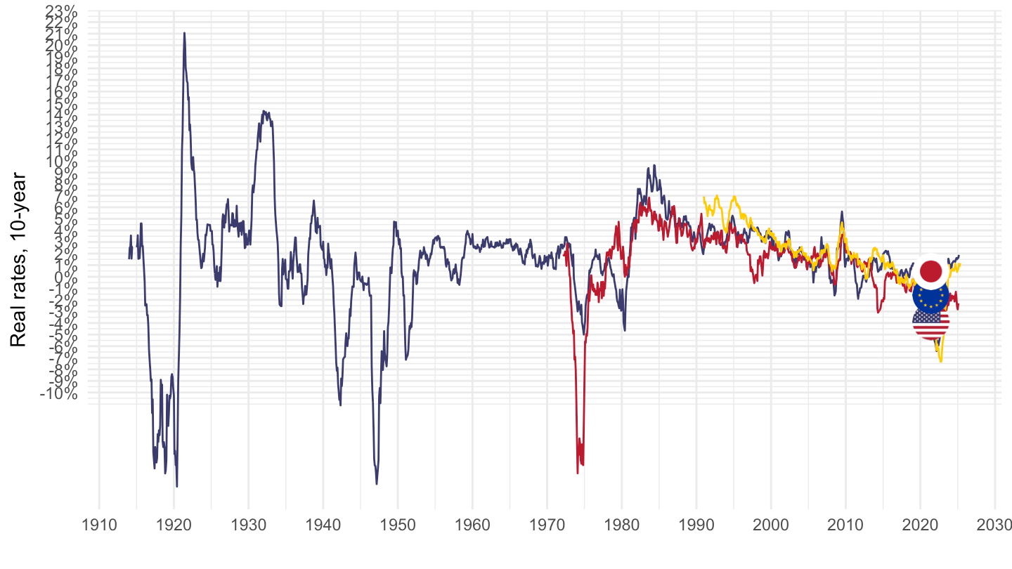
2010-
Code
FM %>%
  filter(PROVIDER_FM_ID %in% c("R_US10YT_RR", "R_JP10YT_RR", "R_U2_10Y")) %>%
  month_to_date %>%
  left_join(REF_AREA, by = "REF_AREA") %>%
  mutate(Ref_area = ifelse(REF_AREA == "U2", "Europe", Ref_area)) %>%
  filter(date >= as.Date("2010-01-01")) %>%
  left_join(colors, by = c("Ref_area" = "country")) %>%
  mutate(color = ifelse(REF_AREA == "U2", color2, color)) %>%
  mutate(OBS_VALUE = OBS_VALUE/100) %>%
  ggplot(.) + theme_minimal() + xlab("") + ylab("Real rates, 10-year") +
  geom_line(aes(x = date, y = OBS_VALUE, color = color)) +
  add_flags(3) + scale_color_identity() +
  scale_x_date(breaks = seq(1960, 2100, 1) %>% paste0("-01-01") %>% as.Date,
               labels = date_format("%Y")) +
  scale_y_continuous(breaks = 0.01*seq(-10, 50, 1),
                     labels = percent_format(accuracy = 1))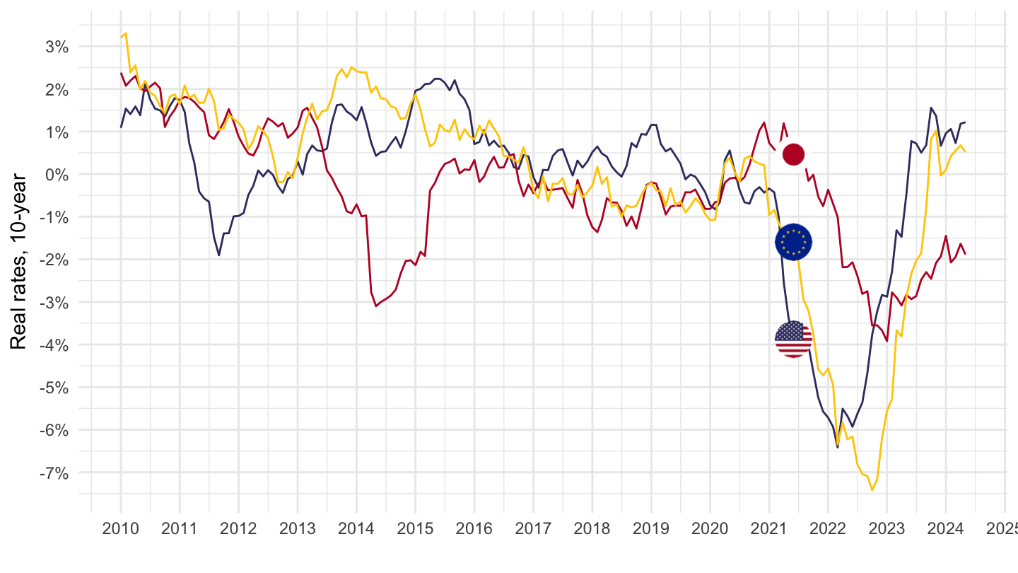
2015-
Code
FM %>%
  filter(PROVIDER_FM_ID %in% c("R_US10YT_RR", "R_JP10YT_RR", "R_U2_10Y")) %>%
  month_to_date %>%
  left_join(REF_AREA, by = "REF_AREA") %>%
  mutate(Ref_area = ifelse(REF_AREA == "U2", "Europe", Ref_area)) %>%
  filter(date >= as.Date("2015-01-01")) %>%
  left_join(colors, by = c("Ref_area" = "country")) %>%
  mutate(color = ifelse(REF_AREA == "U2", color2, color)) %>%
  mutate(OBS_VALUE = OBS_VALUE/100) %>%
  ggplot(.) + theme_minimal() + xlab("") + ylab("Real rates, 10-year") +
  geom_line(aes(x = date, y = OBS_VALUE, color = color)) +
  add_flags(3) + scale_color_identity() +
  scale_x_date(breaks = seq(1960, 2100, 1) %>% paste0("-01-01") %>% as.Date,
               labels = date_format("%Y")) +
  scale_y_continuous(breaks = 0.01*seq(-10, 50, 1),
                     labels = percent_format(accuracy = 1))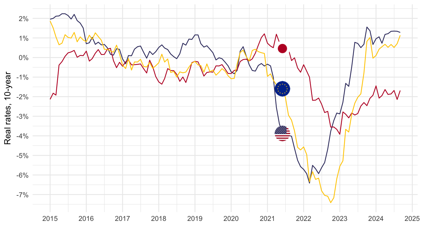
2017-
Code
FM %>%
  filter(PROVIDER_FM_ID %in% c("R_US10YT_RR", "R_JP10YT_RR", "R_U2_10Y")) %>%
  month_to_date %>%
  left_join(REF_AREA, by = "REF_AREA") %>%
  mutate(Ref_area = ifelse(REF_AREA == "U2", "Europe", Ref_area)) %>%
  filter(date >= as.Date("2017-01-01")) %>%
  left_join(colors, by = c("Ref_area" = "country")) %>%
  mutate(color = ifelse(REF_AREA == "U2", color2, color)) %>%
  mutate(OBS_VALUE = OBS_VALUE/100) %>%
  ggplot(.) + theme_minimal() + xlab("") + ylab("Real rates, 10-year") +
  geom_line(aes(x = date, y = OBS_VALUE, color = color)) +
  add_flags(3) + scale_color_identity() +
  scale_x_date(breaks = seq(1960, 2100, 1) %>% paste0("-01-01") %>% as.Date,
               labels = date_format("%Y")) +
  scale_y_continuous(breaks = 0.01*seq(-10, 50, 1),
                     labels = percent_format(accuracy = 1))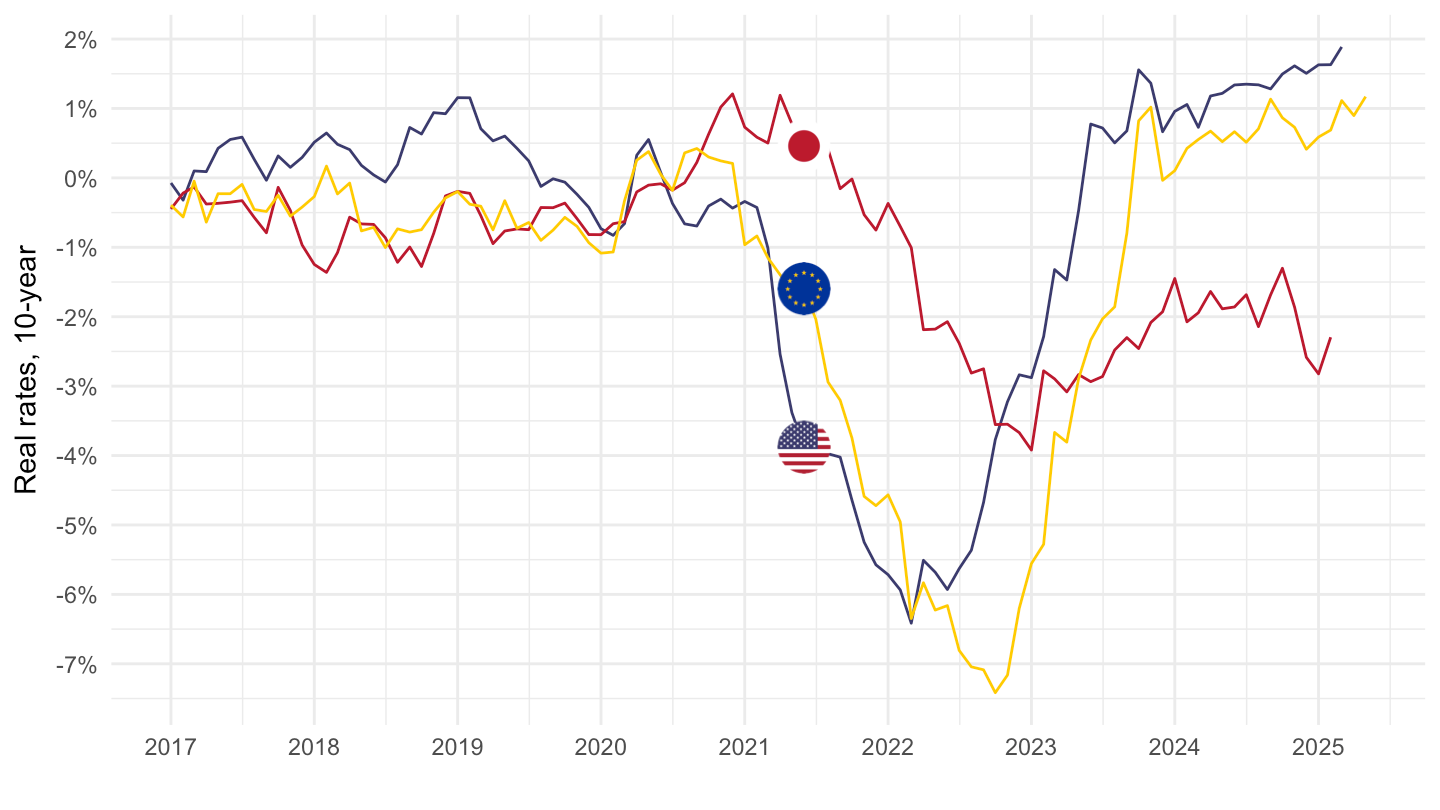
ECB Key Interest rates
EONIA
All
Code
FM %>%
  filter(PROVIDER_FM_ID %in% c("DFR", "MLFR", "MRR_RT", "EONIA"),
         FREQ == "M") %>%
  month_to_date %>%
  left_join(PROVIDER_FM_ID,  by = "PROVIDER_FM_ID") %>%
  ggplot(.) +
  geom_line(aes(x = date, y = OBS_VALUE / 100, color = PROVIDER_FM_ID_desc)) +
  theme_minimal() + xlab("") + ylab("Interest Rates (%)") +
  scale_x_date(breaks = seq(1960, 2025, 2) %>% paste0("-01-01") %>% as.Date,
               labels = date_format("%Y")) +
  scale_y_continuous(breaks = 0.01*seq(-10, 50, 1),
                     labels = percent_format(accuracy = 1)) +
  theme(legend.position = c(0.45, 0.92),
        legend.title = element_blank())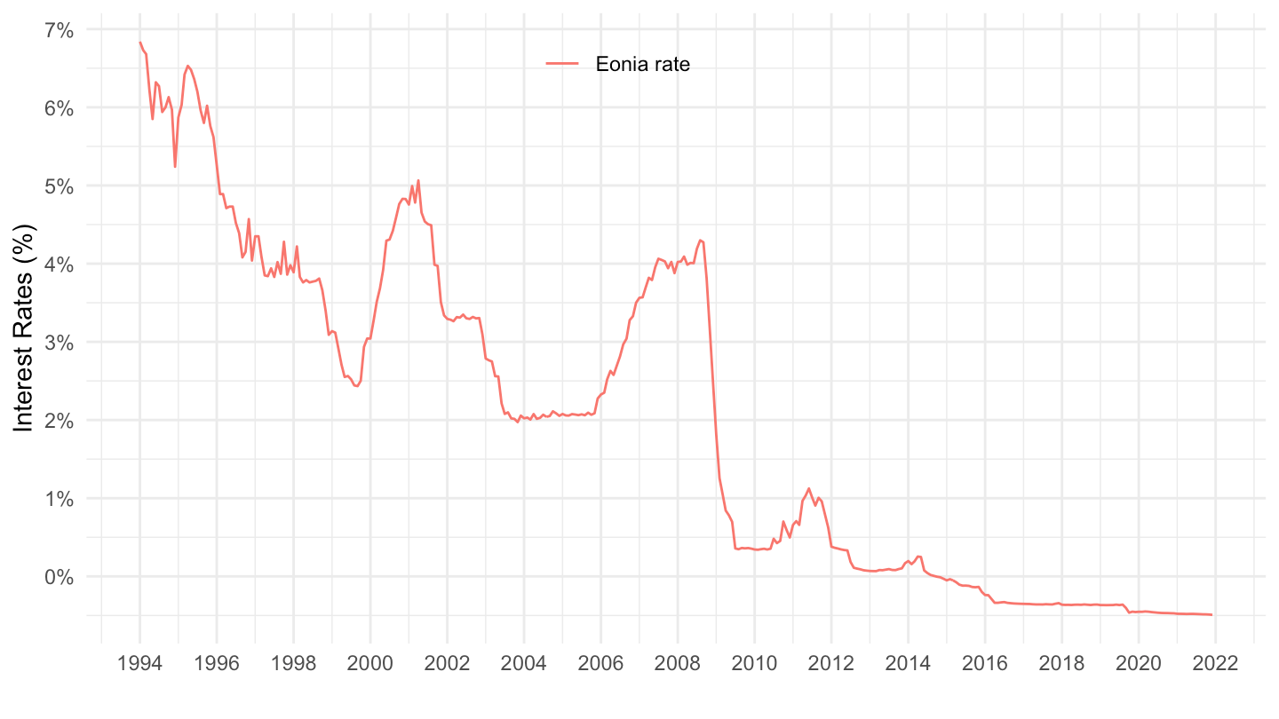
Deposit Facility, Marginal Lending Facility
All
Code
FM %>%
  filter(PROVIDER_FM_ID %in% c("DFR", "MLFR", "MRR_RT", "MRR_FR", "MRR_MBR", "MRR"),
         DATA_TYPE_FM == "LEV",
         FREQ == "D") %>%
  day_to_date %>%
  left_join(PROVIDER_FM_ID,  by = "PROVIDER_FM_ID") %>%
  ggplot(.) +
  geom_line(aes(x = date, y = OBS_VALUE / 100, color = PROVIDER_FM_ID_desc)) +
  theme_minimal() + xlab("") + ylab("Interest Rates (%)") +
  scale_x_date(breaks = seq(1960, 2025, 2) %>% paste0("-01-01") %>% as.Date,
               labels = date_format("%Y")) +
  scale_y_continuous(breaks = 0.01*seq(-10, 50, 1),
                     labels = percent_format(accuracy = 1)) +
  theme(legend.position = c(0.45, 0.92),
        legend.title = element_blank())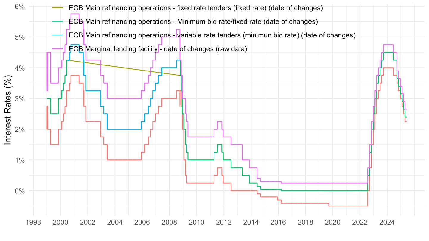
Deposit Facility, Marginal Lending Facility
All
Code
FM %>%
  filter(PROVIDER_FM_ID %in% c("DFR", "MLFR", "MRR_RT"),
         DATA_TYPE_FM == "LEV",
         FREQ == "D") %>%
  day_to_date %>%
  mutate(Provider_fm_id = factor(PROVIDER_FM_ID,
                                 levels = c("MLFR", "MRR_RT", "DFR"),
                                 labels = c("ECB Marginal lending facility",
                                            "ECB Main refinancing operations",
                                            "ECB Deposit facility"))) %>%
  left_join(PROVIDER_FM_ID,  by = "PROVIDER_FM_ID") %>%
  ggplot(.) +
  geom_line(aes(x = date, y = OBS_VALUE / 100, color = Provider_fm_id)) +
  theme_minimal() + xlab("") + ylab("Interest Rates (%)") +
  scale_x_date(breaks = seq(1960, 2025, 2) %>% paste0("-01-01") %>% as.Date,
               labels = date_format("%Y")) +
  scale_y_continuous(breaks = 0.01*seq(-10, 50, 1),
                     labels = percent_format(accuracy = 1)) +
  theme(legend.position = c(0.65, 0.92),
        legend.title = element_blank()) +
  geom_hline(yintercept = 3.75/100, linetype = "dashed")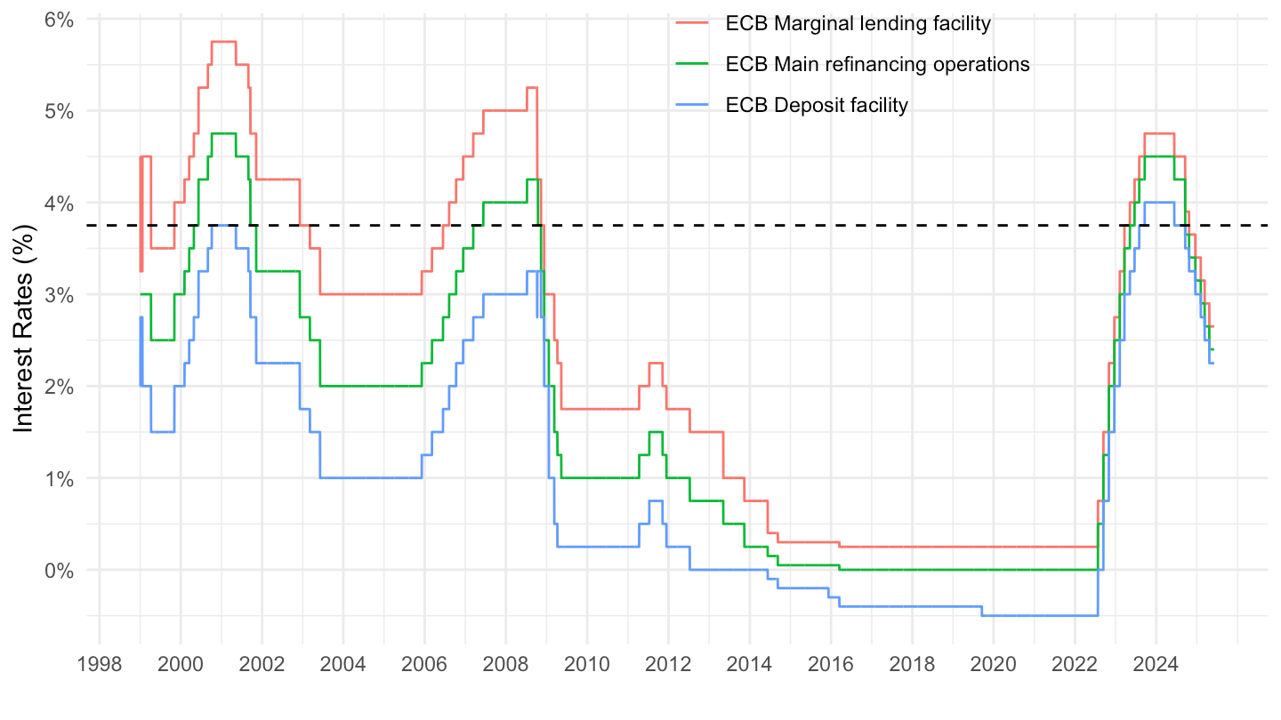
2010
Code
dates_ecb <- FM %>%
  filter(PROVIDER_FM_ID == "DFR") %>%
  day_to_date %>%
  mutate(OBS_VALUE = OBS_VALUE-lag(OBS_VALUE)) %>%
  filter(OBS_VALUE != 0) %>%
  pull(date)
FM %>%
  filter(PROVIDER_FM_ID %in% c("DFR", "MLFR", "MRR_RT"),
         DATA_TYPE_FM == "LEV",
         FREQ == "D") %>%
  day_to_date %>%
  left_join(PROVIDER_FM_ID,  by = "PROVIDER_FM_ID") %>%
  mutate(Provider_fm_id = factor(PROVIDER_FM_ID,
                                 levels = c("MLFR", "MRR_RT", "DFR"),
                                 labels = c("ECB Marginal lending facility",
                                            "ECB Main refinancing operations - Minimum bid rate/fixed rate",
                                            "ECB Deposit facility"))) %>%
  filter(date >= as.Date("2010-01-01"))%>%
  ggplot(.) +
  geom_line(aes(x = date, y = OBS_VALUE / 100, color = Provider_fm_id)) +
  theme_minimal() + xlab("") + ylab("Interest Rates (%)") +
  scale_x_date(breaks = dates_ecb,
               labels = date_format("%Y")) +
  scale_y_continuous(breaks = 0.01*seq(-10, 50, 0.5),
                     labels = percent_format(accuracy = .1)) +
  theme(legend.position = c(0.45, 0.92),
        legend.title = element_blank())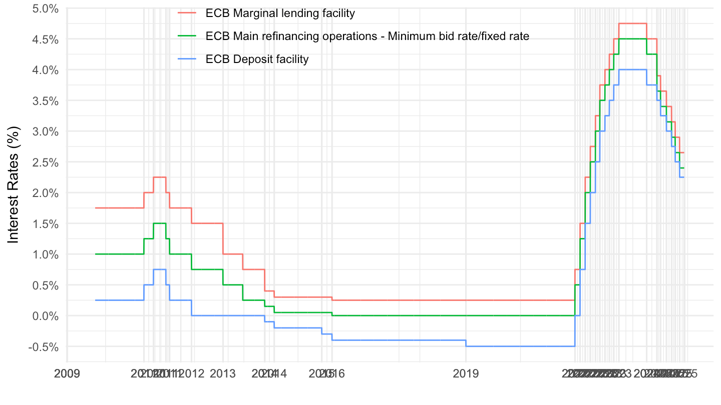
2016-
Code
FM %>%
  filter(PROVIDER_FM_ID %in% c("DFR", "MLFR", "MRR_RT"),
         DATA_TYPE_FM == "LEV",
         FREQ == "D") %>%
  day_to_date %>%
  left_join(PROVIDER_FM_ID,  by = "PROVIDER_FM_ID") %>%
  filter(date >= as.Date("2016-01-01"))%>%
  mutate(Provider_fm_id = factor(PROVIDER_FM_ID,
                                 levels = c("MLFR", "MRR_RT", "DFR"),
                                 labels = c("ECB Marginal lending facility",
                                            "ECB Main refinancing operations - Minimum bid rate/fixed rate",
                                            "ECB Deposit facility"))) %>%
  ggplot(.) +
  geom_line(aes(x = date, y = OBS_VALUE / 100, color = Provider_fm_id)) +
  theme_minimal() + xlab("") + ylab("Interest Rates (%)") +
  scale_x_date(breaks = seq(1960, 2025, 1) %>% paste0("-01-01") %>% as.Date,
               labels = date_format("%Y")) +
  scale_y_continuous(breaks = 0.01*seq(-10, 50, 1),
                     labels = percent_format(accuracy = 1)) +
  theme(legend.position = c(0.45, 0.92),
        legend.title = element_blank())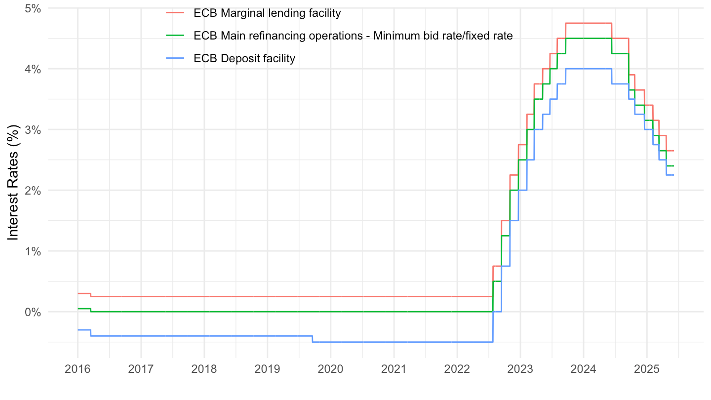
2022-
Code
FM %>%
  filter(PROVIDER_FM_ID %in% c("DFR", "MLFR", "MRR_RT"),
         DATA_TYPE_FM == "LEV",
         FREQ == "D") %>%
  day_to_date %>%
  filter(date >= as.Date("2022-01-01")) %>%
  add_row(date = as.Date("2025-06-11"), PROVIDER_FM_ID = "DFR", OBS_VALUE = 2) %>%
  add_row(date = as.Date("2025-06-11"), PROVIDER_FM_ID = "MRR_RT", OBS_VALUE = 2.15) %>%
  add_row(date = as.Date("2025-06-11"), PROVIDER_FM_ID = "MLFR", OBS_VALUE = 2.4) %>%
  add_row(date = as.Date("2025-06-10"), PROVIDER_FM_ID = "DFR", OBS_VALUE = 2.25) %>%
  add_row(date = as.Date("2025-06-10"), PROVIDER_FM_ID = "MRR_RT", OBS_VALUE = 2.4) %>%
  add_row(date = as.Date("2025-06-10"), PROVIDER_FM_ID = "MLFR", OBS_VALUE = 2.65) %>%
  arrange(desc(date)) %>%
  #add_row(date = as.Date("2024-09-17"), PROVIDER_FM_ID = "DFR", OBS_VALUE = 3.5) %>%
  #add_row(date = as.Date("2024-09-17"), PROVIDER_FM_ID = "MRR_RT", OBS_VALUE = 3.65) %>%
  #add_row(date = as.Date("2024-09-17"), PROVIDER_FM_ID = "MLFR", OBS_VALUE = 3.9) %>%
  left_join(PROVIDER_FM_ID,  by = "PROVIDER_FM_ID") %>%
  mutate(Provider_fm_id = factor(PROVIDER_FM_ID,
                                 levels = c("MLFR", "MRR_RT", "DFR"),
                                 labels = c("ECB Marginal lending facility",
                                            "ECB Main refinancing operations - Minimum bid rate/fixed rate",
                                            "ECB Deposit facility"))) %>%
  ggplot(.) +
  geom_line(aes(x = date, y = OBS_VALUE / 100, color = Provider_fm_id)) +
  theme_minimal() + xlab("") + ylab("Interest Rates (%)") +
  scale_x_date(breaks = c(dates_ecb),
               labels = date_format("%d %B %Y")) +
  scale_y_continuous(breaks = 0.01*seq(-10, 50, 0.5),
                     labels = percent_format(accuracy = .1)) +
  theme(legend.position = c(0.65, 0.2),
        legend.title = element_blank(),
        axis.text.x = element_text(angle = 45, vjust = 1, hjust = 1)) +
  geom_label_repel(data = . %>% filter(date == max(date)),
                   aes(x = date, y = OBS_VALUE / 100, label = percent(OBS_VALUE / 100, acc = 0.01), color = Provider_fm_id))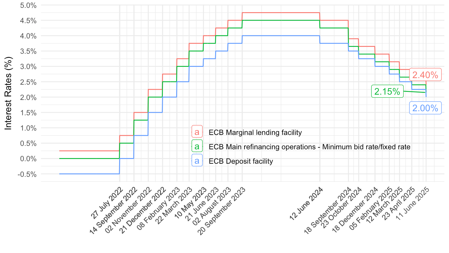
2022 - Dates of change
Schedules for the meetings of the Governing Council. html
Key ECB interest rates: Dates of change. html
Code
FM %>%
  filter(PROVIDER_FM_ID %in% c("DFR", "MLFR", "MRR_RT"),
         DATA_TYPE_FM == "LEV",
         FREQ == "D") %>%
  day_to_date %>%
  left_join(PROVIDER_FM_ID,  by = "PROVIDER_FM_ID") %>%
  mutate(Provider_fm_id = factor(PROVIDER_FM_ID,
                                 levels = c("MLFR", "MRR_RT", "DFR"),
                                 labels = c("ECB Marginal lending facility",
                                            "ECB Main refinancing operations",
                                            "ECB Deposit facility"))) %>%
  filter(date >= as.Date("2022-07-01")) %>%
  ggplot(.) +
  geom_line(aes(x = date, y = OBS_VALUE / 100, color = Provider_fm_id)) +
  theme_minimal() + xlab("") + ylab("Interest Rates (%)") +
  scale_x_date(breaks = c(dates_ecb, Sys.Date()),
               labels = date_format("%d %B %Y")) +
  scale_y_continuous(breaks = 0.01*seq(-10, 50, 0.5),
                     labels = percent_format(accuracy = .1)) +
  theme(legend.position = c(0.7, 0.2),
        legend.title = element_blank(),
        axis.text.x = element_text(angle = 45, vjust = 1, hjust = 1))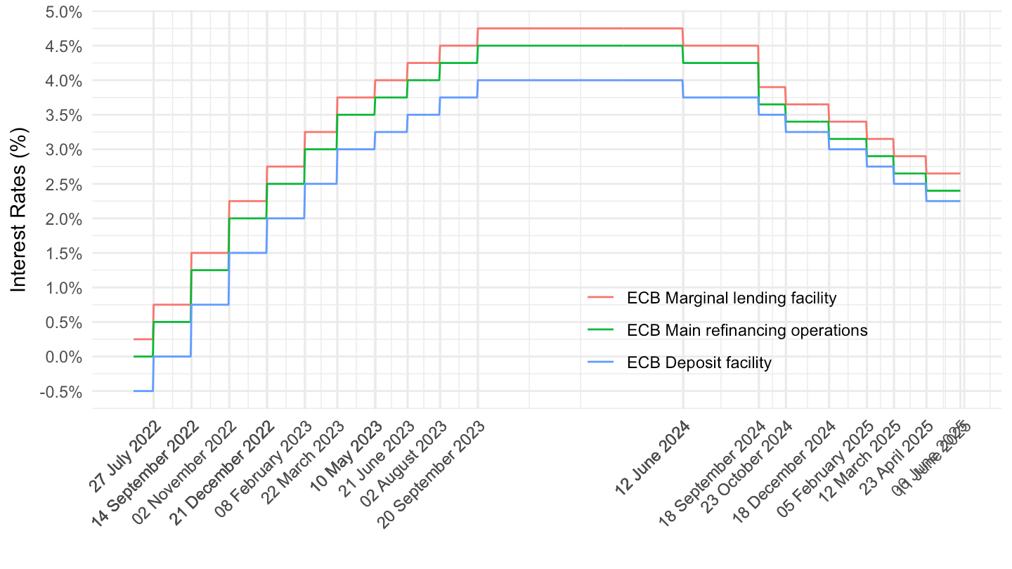
Around September 2022
Code
FM %>%
  filter(PROVIDER_FM_ID %in% c("DFR", "MLFR", "MRR_RT"),
         DATA_TYPE_FM == "LEV",
         FREQ == "D") %>%
  day_to_date %>%
  left_join(PROVIDER_FM_ID,  by = "PROVIDER_FM_ID") %>%
  filter(date >= as.Date("2022-09-05"),
         date <= as.Date("2022-09-20")) %>%
  ggplot(.) +
  geom_line(aes(x = date, y = OBS_VALUE / 100, color = PROVIDER_FM_ID_desc)) +
  theme_minimal() + xlab("") + ylab("Interest Rates (%)") +
  scale_x_date(breaks = seq(from = as.Date("2022-01-01"), as.Date("2026-01-01"), by = "1 day"),
               labels = date_format("%d %b %Y")) +
  scale_y_continuous(breaks = 0.01*seq(-10, 50, 0.25),
                     labels = percent_format(accuracy = .01)) +
  theme(legend.position = c(0.4, 0.92),
        legend.title = element_blank(),
        axis.text.x = element_text(angle = 45, vjust = 1, hjust = 1))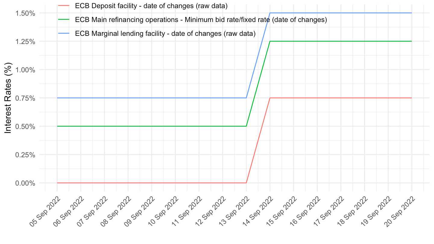
Japan
1970-
Code
FM %>%
  filter(PROVIDER_FM_ID %in% c("JP10YT_RR", "R_JP10YT_RR")) %>%
  month_to_date %>%
  left_join(PROVIDER_FM_ID,  by = "PROVIDER_FM_ID") %>%
  ggplot(.) +
  geom_line(aes(x = date, y = OBS_VALUE / 100, color = PROVIDER_FM_ID_desc)) +
  theme_minimal() + xlab("") + ylab("Interest Rates (%)") +
  scale_x_date(breaks = seq(1960, 2100, 5) %>% paste0("-01-01") %>% as.Date,
               labels = date_format("%Y")) +
  scale_y_continuous(breaks = 0.01*seq(-50, 50, 2),
                     labels = percent_format(accuracy = 1)) +
  theme(legend.position = c(0.75, 0.9),
        legend.title = element_blank())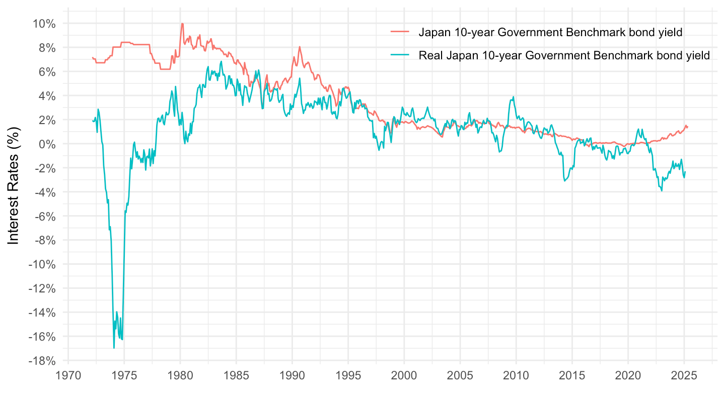
2000-
Code
FM %>%
  filter(PROVIDER_FM_ID %in% c("JP10YT_RR", "R_JP10YT_RR")) %>%
  month_to_date %>%
  filter(date >= as.Date("2000-01-01")) %>%
  left_join(PROVIDER_FM_ID,  by = "PROVIDER_FM_ID") %>%
  ggplot(.) +
  geom_line(aes(x = date, y = OBS_VALUE / 100, color = PROVIDER_FM_ID_desc)) +
  theme_minimal() + xlab("") + ylab("Interest Rates (%)") +
  scale_x_date(breaks = seq(1960, 2100, 2) %>% paste0("-01-01") %>% as.Date,
               labels = date_format("%Y")) +
  scale_y_continuous(breaks = 0.01*seq(-50, 50, 1),
                     labels = percent_format(accuracy = 1)) +

  theme(legend.position = c(0.75, 0.9),
        legend.title = element_blank())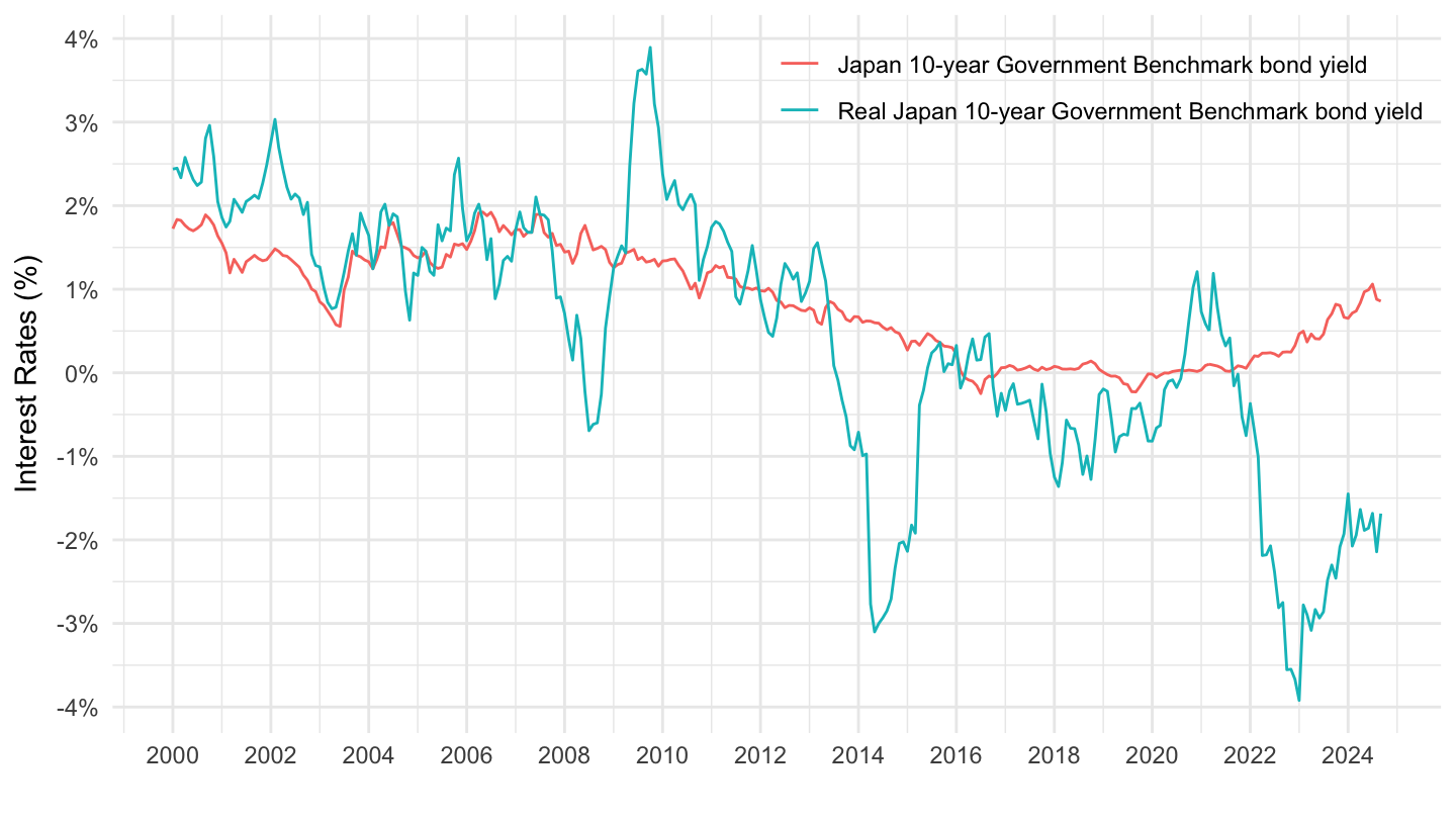
United States
1970-
Code
FM %>%
  filter(PROVIDER_FM_ID %in% c("US10YT_RR", "R_US10YT_RR")) %>%
  month_to_date %>%
  left_join(PROVIDER_FM_ID,  by = "PROVIDER_FM_ID") %>%
  ggplot(.) +
  geom_line(aes(x = date, y = OBS_VALUE / 100, color = PROVIDER_FM_ID_desc)) +
  theme_minimal() + xlab("") + ylab("Interest Rates (%)") +
  scale_x_date(breaks = seq(1900, 2100, 10) %>% paste0("-01-01") %>% as.Date,
               labels = date_format("%Y")) +
  scale_y_continuous(breaks = 0.01*seq(-50, 50, 2),
                     labels = percent_format(accuracy = 1)) +

  theme(legend.position = c(0.75, 0.9),
        legend.title = element_blank())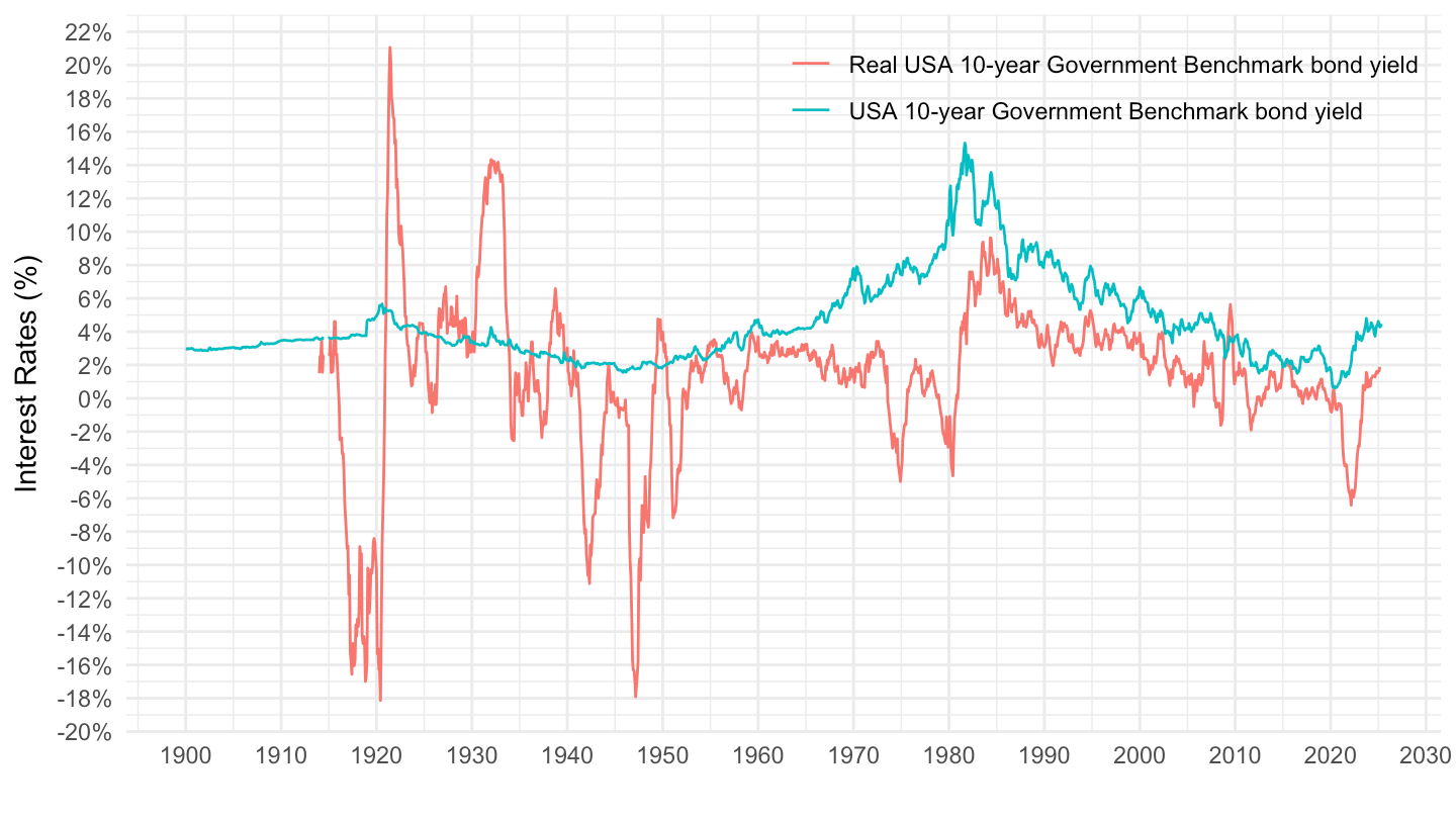
2000-
Code
FM %>%
  filter(PROVIDER_FM_ID %in% c("US10YT_RR", "R_US10YT_RR")) %>%
  month_to_date %>%
  filter(date >= as.Date("2000-01-01")) %>%
  left_join(PROVIDER_FM_ID,  by = "PROVIDER_FM_ID") %>%
  ggplot(.) +
  geom_line(aes(x = date, y = OBS_VALUE / 100, color = PROVIDER_FM_ID_desc)) +
  theme_minimal() + xlab("") + ylab("Interest Rates (%)") +
  scale_x_date(breaks = seq(1960, 2100, 2) %>% paste0("-01-01") %>% as.Date,
               labels = date_format("%Y")) +
  scale_y_continuous(breaks = 0.01*seq(-50, 50, 1),
                     labels = percent_format(accuracy = 1)) +

  theme(legend.position = c(0.75, 0.9),
        legend.title = element_blank())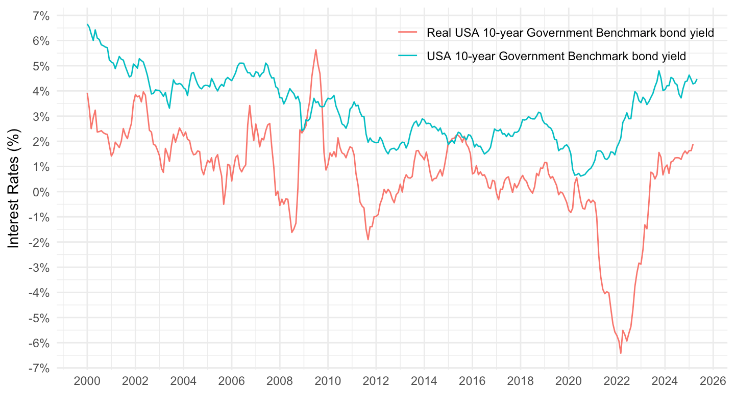
Euro area
1970-
Code
FM %>%
  filter(PROVIDER_FM_ID %in% c("U2_10Y", "R_U2_10Y")) %>%
  month_to_date %>%
  left_join(PROVIDER_FM_ID,  by = "PROVIDER_FM_ID") %>%
  ggplot(.) +
  geom_line(aes(x = date, y = OBS_VALUE / 100, color = PROVIDER_FM_ID_desc)) +
  theme_minimal() + xlab("") + ylab("Interest Rates (%)") +
  scale_x_date(breaks = seq(1900, 2100, 10) %>% paste0("-01-01") %>% as.Date,
               labels = date_format("%Y")) +
  scale_y_continuous(breaks = 0.01*seq(-50, 50, 2),
                     labels = percent_format(accuracy = 1)) +

  theme(legend.position = c(0.75, 0.9),
        legend.title = element_blank())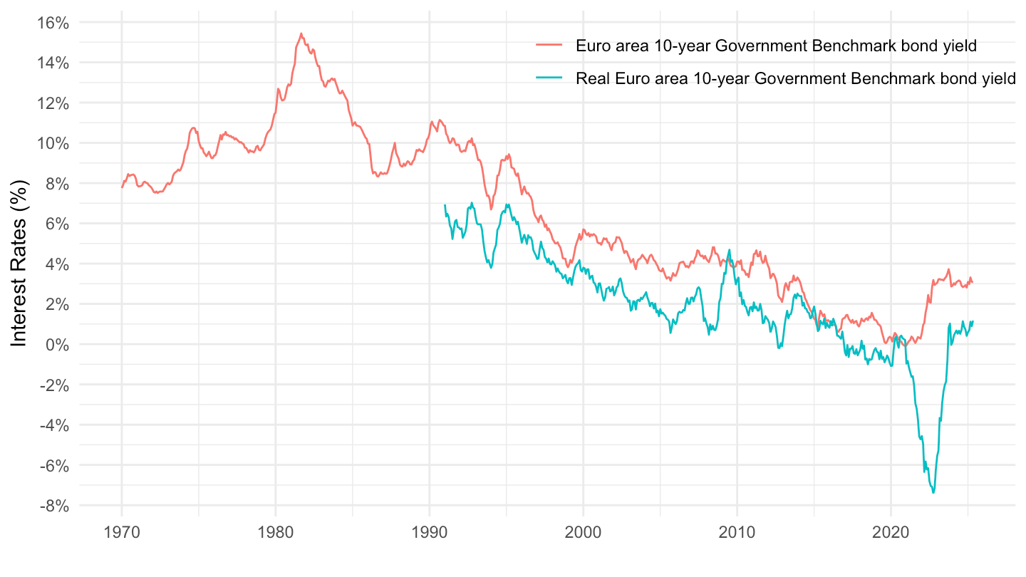
2000-
Code
FM %>%
  filter(PROVIDER_FM_ID %in% c("U2_10Y", "R_U2_10Y")) %>%
  month_to_date %>%
  filter(date >= as.Date("2000-01-01")) %>%
  left_join(PROVIDER_FM_ID,  by = "PROVIDER_FM_ID") %>%
  ggplot(.) +
  geom_line(aes(x = date, y = OBS_VALUE / 100, color = PROVIDER_FM_ID_desc)) +
  theme_minimal() + xlab("") + ylab("Interest Rates (%)") +
  scale_x_date(breaks = seq(1960, 2100, 2) %>% paste0("-01-01") %>% as.Date,
               labels = date_format("%Y")) +
  scale_y_continuous(breaks = 0.01*seq(-50, 50, 1),
                     labels = percent_format(accuracy = 1)) +

  theme(legend.position = c(0.35, 0.2),
        legend.title = element_blank())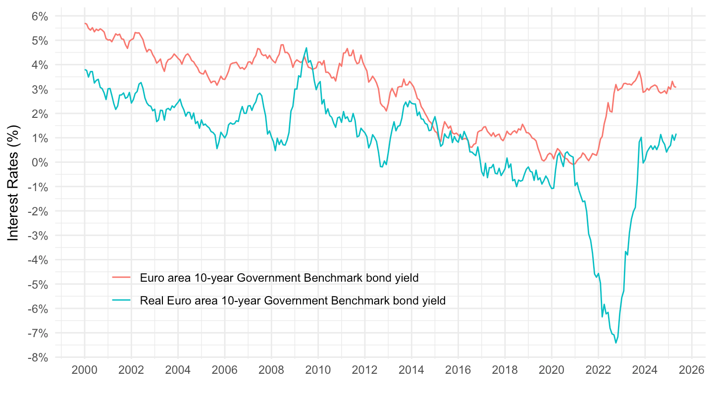
2015-
Code
FM %>%
  filter(PROVIDER_FM_ID %in% c("U2_10Y", "R_U2_10Y")) %>%
  month_to_date %>%
  filter(date >= as.Date("2015-01-01")) %>%
  left_join(PROVIDER_FM_ID,  by = "PROVIDER_FM_ID") %>%
  ggplot(.) +
  geom_line(aes(x = date, y = OBS_VALUE / 100, color = PROVIDER_FM_ID_desc)) +
  theme_minimal() + xlab("") + ylab("Interest Rates (%)") +
  scale_x_date(breaks = seq(1960, 2100, 1) %>% paste0("-01-01") %>% as.Date,
               labels = date_format("%Y")) +
  scale_y_continuous(breaks = 0.01*seq(-50, 50, 1),
                     labels = percent_format(accuracy = 1)) +

  theme(legend.position = c(0.35, 0.2),
        legend.title = element_blank())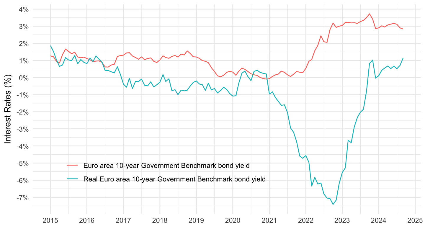
More…
Data on monetary policy
| source | dataset | Title | .html | .rData |
|---|---|---|---|---|
| bdf | FM | Marché financier, taux | 2026-07-22 | 2026-07-22 |
| ecb | FM | Financial market data | 2026-07-23 | 2026-07-22 |
| bdf | MIR | Taux d'intérêt - Zone euro | 2026-07-22 | 2026-07-22 |
| bdf | MIR1 | Taux d'intérêt - France | 2026-07-23 | 2026-07-23 |
| bis | CBPOL | Policy Rates, Daily | 2026-07-18 | 2026-07-22 |
| ecb | BSI | Balance Sheet Items | 2026-07-23 | 2026-07-22 |
| ecb | BSI_PUB | Balance Sheet Items - Published series | 2026-07-23 | 2026-07-22 |
| ecb | ILM | Internal Liquidity Management | 2026-07-23 | 2026-07-22 |
| ecb | ILM_PUB | Internal Liquidity Management - Published series | 2026-07-23 | 2026-07-22 |
| ecb | MIR | MFI Interest Rate Statistics | 2026-07-23 | 2026-07-22 |
| ecb | RAI | Risk Assessment Indicators | 2026-07-23 | 2026-07-23 |
| ecb | SUP | Supervisory Banking Statistics | 2026-07-23 | 2026-07-23 |
| ecb | YC | Financial market data - yield curve | 2026-07-23 | 2026-07-23 |
| ecb | YC_PUB | Financial market data - yield curve - Published series | 2026-07-23 | 2026-07-23 |
| ecb | liq_daily | Daily Liquidity | 2026-07-23 | 2026-07-23 |
| eurostat | ei_mfir_m | Interest rates - monthly data | 2026-07-23 | 2026-07-23 |
| eurostat | irt_st_m | Money market interest rates - monthly data | 2026-07-23 | 2026-07-23 |
| fred | r | Interest Rates | 2026-07-22 | 2026-07-22 |
| oecd | MEI | Main Economic Indicators | 2024-04-16 | 2025-07-24 |
| oecd | MEI_FIN | Monthly Monetary and Financial Statistics (MEI) | 2024-09-15 | 2025-07-24 |
Data on interest rates
| source | dataset | Title | .html | .rData |
|---|---|---|---|---|
| bdf | FM | Marché financier, taux | 2026-07-22 | 2026-07-22 |
| ecb | FM | Financial market data | 2026-07-23 | 2026-07-22 |
| bdf | MIR | Taux d'intérêt - Zone euro | 2026-07-22 | 2026-07-22 |
| bdf | MIR1 | Taux d'intérêt - France | 2026-07-23 | 2026-07-23 |
| bis | CBPOL_D | Policy Rates, Daily | 2026-07-18 | 2025-08-20 |
| bis | CBPOL_M | Policy Rates, Monthly | 2026-07-22 | 2024-04-19 |
| ecb | MIR | MFI Interest Rate Statistics | 2026-07-23 | 2026-07-22 |
| eurostat | ei_mfir_m | Interest rates - monthly data | 2026-07-23 | 2026-07-23 |
| eurostat | irt_lt_mcby_d | EMU convergence criterion series - daily data | 2026-07-23 | 2025-07-24 |
| eurostat | irt_st_m | Money market interest rates - monthly data | 2026-07-23 | 2026-07-23 |
| fred | r | Interest Rates | 2026-07-22 | 2026-07-22 |
| oecd | MEI | Main Economic Indicators | 2024-04-16 | 2025-07-24 |
| oecd | MEI_FIN | Monthly Monetary and Financial Statistics (MEI) | 2024-09-15 | 2025-07-24 |
| wdi | FR.INR.DPST | Deposit interest rate (%) | 2022-09-27 | 2026-07-22 |
| wdi | FR.INR.LEND | Lending interest rate (%) | 2026-07-22 | 2026-07-22 |
| wdi | FR.INR.RINR | Real interest rate (%) | 2026-01-11 | 2026-07-22 |