Policy Rates, Daily
Data - BIS
Info
LAST_COMPILE
| LAST_COMPILE |
|---|
| 2026-07-25 |
Last
| date | Nobs |
|---|---|
| 2026-07-21 | 15 |
iso3c, REF_AREA, Reference area
Code
CBPOL_D %>%

  left_join(REF_AREA, by = "REF_AREA") %>%
  group_by(REF_AREA, `Reference area`) %>%
  summarise(Nobs = n(),
            start = first(date),
            end = last(date)) %>%
  arrange(-Nobs) %>%
  mutate(Flag = gsub(" ", "-", str_to_lower(`Reference area`)),
         Flag = paste0('<img src="../../icon/flag/vsmall/', Flag, '.png" alt="Flag">')) %>%
  select(Flag, everything()) %>%
  {if (is_html_output()) datatable(., filter = 'top', rownames = F, escape = F) else .}
FREQ, Freq
Code
CBPOL_D %>%
  left_join(FREQ, by = "FREQ") %>%
  group_by(FREQ, Freq) %>%
  summarise(Nobs = n()) %>%
  arrange(-Nobs) %>%
{if (is_html_output()) print_table(.) else .}| FREQ | Freq | Nobs |
|---|---|---|
| D | Daily | 636384 |
Individual Countries
Poland
All
Code
CBPOL_D %>%

  left_join(REF_AREA, by = "REF_AREA") %>%
  filter(REF_AREA %in% c("PL")) %>%
  ggplot(.) + geom_line(aes(x = date, y = value/100)) +
  theme_minimal() + xlab("") + ylab("") +
  scale_x_date(breaks = seq(1940, 2100, 2) %>% paste0("-01-01") %>% as.Date,
               labels = date_format("%Y")) +
  scale_y_continuous(breaks = 0.01*seq(0, 10000, 1),
                labels = percent_format(accuracy = 1)) +
  scale_color_manual(values = viridis(4)[1:3]) +
  theme(legend.position = c(0.8, 0.80),
        legend.title = element_blank())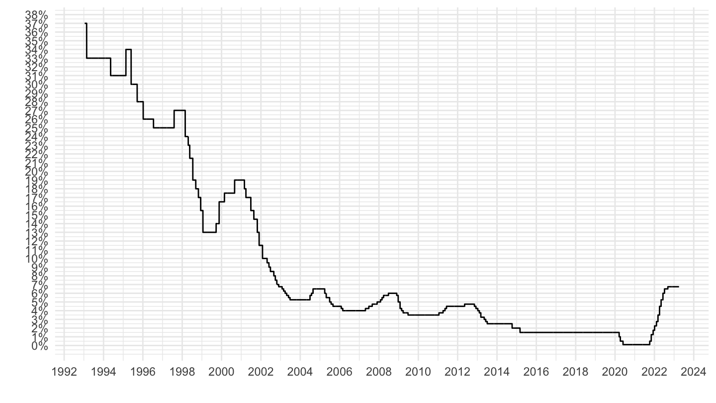
1999-
Code
CBPOL_D %>%

  left_join(REF_AREA, by = "REF_AREA") %>%
  filter(REF_AREA %in% c("PL"),
         date >= as.Date("1999-01-01")) %>%
  ggplot(.) + geom_line(aes(x = date, y = value/100)) +
  theme_minimal() + xlab("") + ylab("") +
  scale_x_date(breaks = seq(1940, 2100, 2) %>% paste0("-01-01") %>% as.Date,
               labels = date_format("%Y")) +
  scale_y_continuous(breaks = 0.01*seq(0, 10000, 1),
                labels = percent_format(accuracy = 1)) +
  scale_color_manual(values = viridis(4)[1:3]) +
  theme(legend.position = c(0.8, 0.80),
        legend.title = element_blank())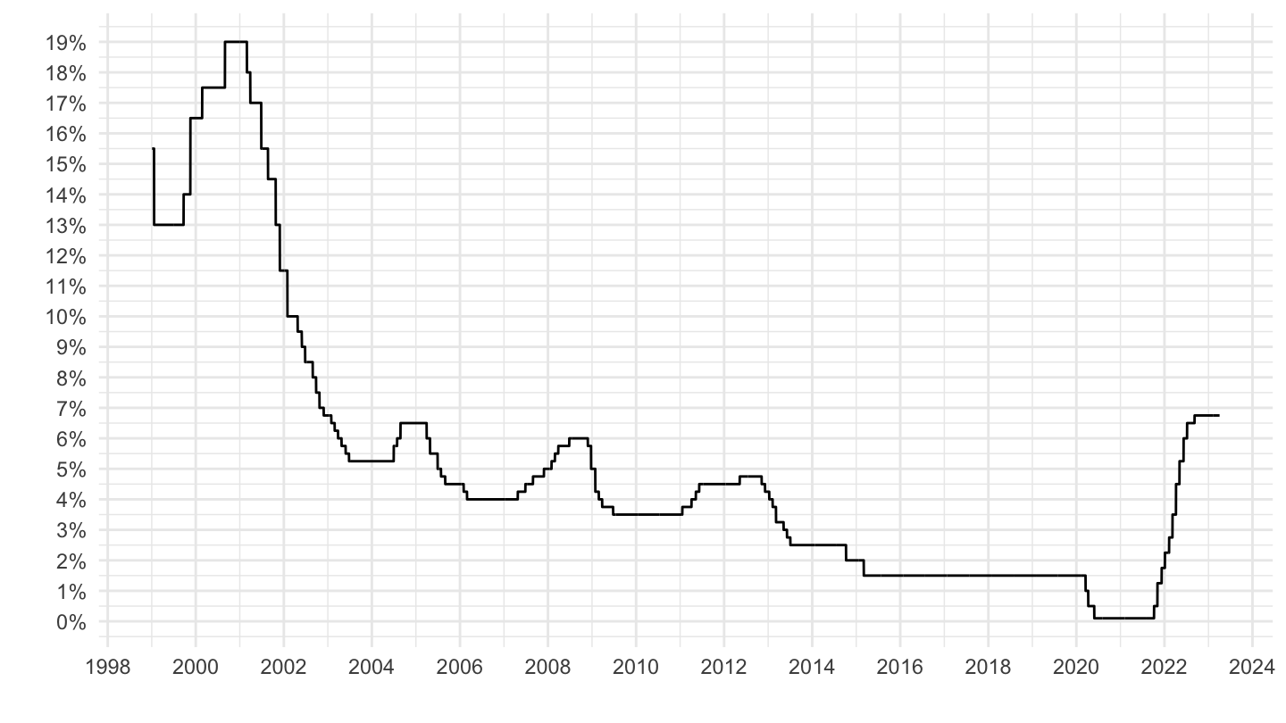
2003-
Code
CBPOL_D %>%

  left_join(REF_AREA, by = "REF_AREA") %>%
  filter(REF_AREA %in% c("PL"),
         date >= as.Date("2003-01-01")) %>%
  ggplot(.) + geom_line(aes(x = date, y = value/100)) +
  theme_minimal() + xlab("") + ylab("") +
  scale_x_date(breaks = seq(1940, 2100, 2) %>% paste0("-01-01") %>% as.Date,
               labels = date_format("%Y")) +
  scale_y_continuous(breaks = 0.01*seq(0, 10000, 1),
                labels = percent_format(accuracy = 1)) +
  scale_color_manual(values = viridis(4)[1:3]) +
  theme(legend.position = c(0.8, 0.80),
        legend.title = element_blank())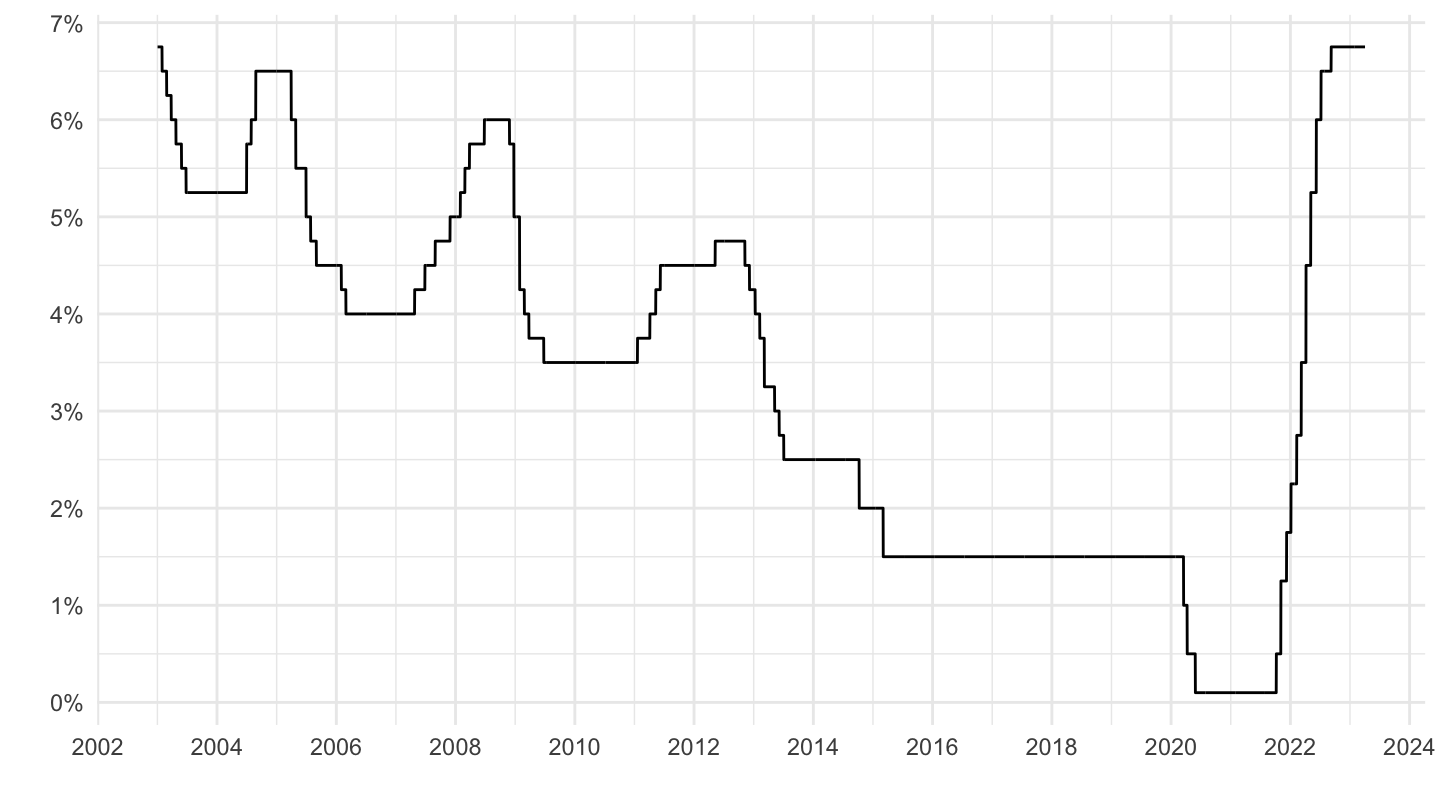
Iceland
All
Code
CBPOL_D %>%

  left_join(REF_AREA, by = "REF_AREA") %>%
  filter(REF_AREA %in% c("IS")) %>%
  ggplot(.) + geom_line(aes(x = date, y = value/100)) +
  theme_minimal() + xlab("") + ylab("") +
  scale_x_date(breaks = seq(1940, 2100, 2) %>% paste0("-01-01") %>% as.Date,
               labels = date_format("%Y")) +
  scale_y_continuous(breaks = 0.01*seq(0, 10000, 1),
                labels = percent_format(accuracy = 1)) +
  scale_color_manual(values = viridis(4)[1:3]) +
  theme(legend.position = c(0.8, 0.80),
        legend.title = element_blank())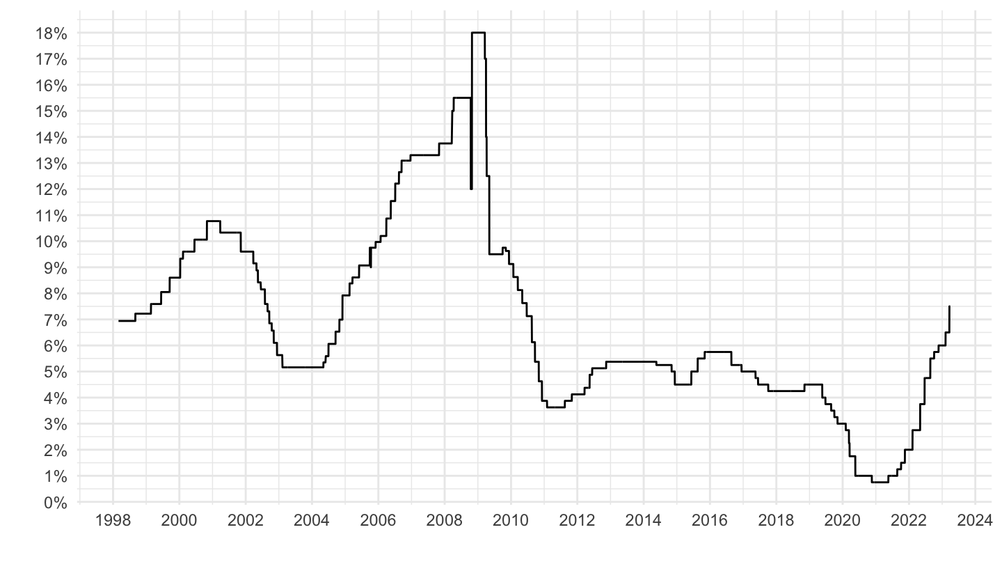
Israel
All
Code
CBPOL_D %>%

  left_join(REF_AREA, by = "REF_AREA") %>%
  filter(REF_AREA %in% c("IL")) %>%
  ggplot(.) + geom_line(aes(x = date, y = value/100)) +
  theme_minimal() + xlab("") + ylab("") +
  scale_x_date(breaks = seq(1940, 2100, 5) %>% paste0("-01-01") %>% as.Date,
               labels = date_format("%Y")) +
  scale_y_continuous(breaks = 0.01*seq(0, 10000, 1),
                labels = percent_format(accuracy = 1)) +
  scale_color_manual(values = viridis(4)[1:3]) +
  theme(legend.position = c(0.8, 0.80),
        legend.title = element_blank())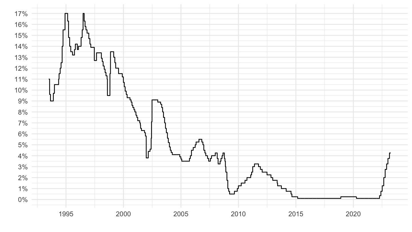
All - Stanley Fischer
Code
CBPOL_D %>%

  left_join(REF_AREA, by = "REF_AREA") %>%
  filter(REF_AREA %in% c("IL")) %>%
  ggplot(.) + geom_line(aes(x = date, y = value/100)) +
  theme_minimal() + xlab("") + ylab("") +
  scale_x_date(breaks = seq(1940, 2100, 5) %>% paste0("-01-01") %>% as.Date,
               labels = date_format("%Y")) +
  scale_y_continuous(breaks = 0.01*seq(0, 10000, 1),
                labels = percent_format(accuracy = 1)) +
  scale_color_manual(values = viridis(4)[1:3]) +
  theme(legend.position = c(0.8, 0.80),
        legend.title = element_blank()) +
    geom_rect(data = data_frame(start = as.Date("2005-05-01"),
                                end = as.Date("2013-06-30")),
              aes(xmin = start, xmax = end, ymin = -Inf, ymax = +Inf),
              fill = viridis(4)[4], alpha = 0.2)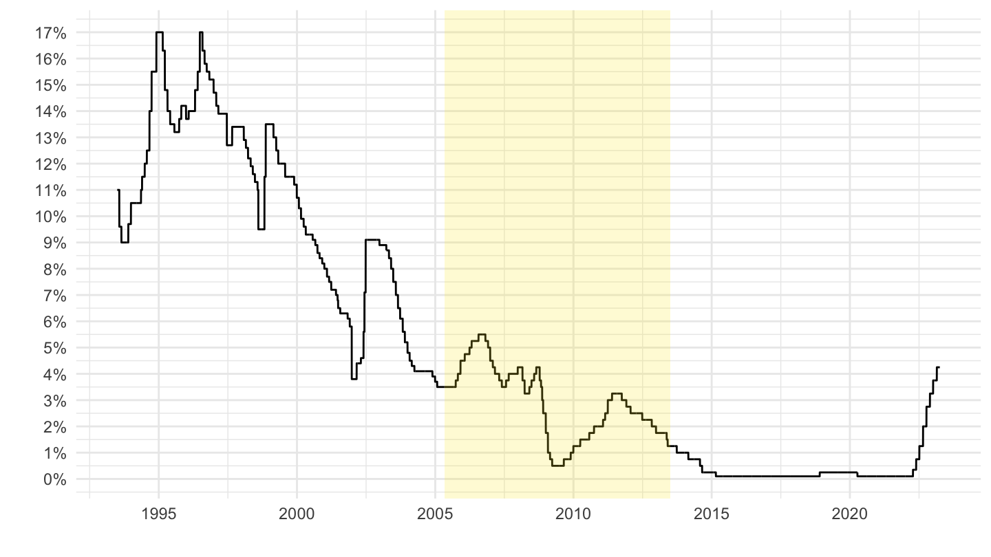
2004-
Code
CBPOL_D %>%

  left_join(REF_AREA, by = "REF_AREA") %>%
  filter(REF_AREA %in% c("IL"),
         date >= as.Date("2004-01-01")) %>%
  ggplot(.) + geom_line(aes(x = date, y = value/100)) +
  theme_minimal() + xlab("") + ylab("") +
  scale_x_date(breaks = seq(1940, 2100, 2) %>% paste0("-01-01") %>% as.Date,
               labels = date_format("%Y")) +
  scale_y_continuous(breaks = 0.01*seq(0, 10000, 1),
                labels = percent_format(accuracy = 1)) +
  scale_color_manual(values = viridis(4)[1:3]) +
  theme(legend.position = c(0.8, 0.80),
        legend.title = element_blank())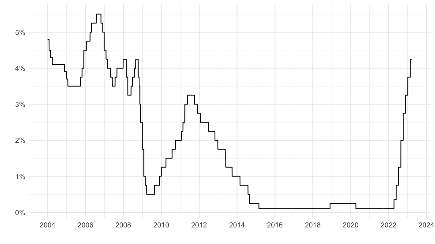
2004- Stanley Fischer
Code
CBPOL_D %>%

  left_join(REF_AREA, by = "REF_AREA") %>%
  filter(REF_AREA %in% c("IL"),
         date >= as.Date("2004-01-01")) %>%
  ggplot(.) + geom_line(aes(x = date, y = value/100)) +
  theme_minimal() + xlab("") + ylab("") +
  scale_x_date(breaks = seq(1940, 2100, 2) %>% paste0("-01-01") %>% as.Date,
               labels = date_format("%Y")) +
  scale_y_continuous(breaks = 0.01*seq(0, 10000, 1),
                labels = percent_format(accuracy = 1)) +
  scale_color_manual(values = viridis(4)[1:3]) +
  theme(legend.position = c(0.8, 0.80),
        legend.title = element_blank()) +
    geom_rect(data = data_frame(start = as.Date("2005-05-01"),
                                end = as.Date("2013-06-30")),
              aes(xmin = start, xmax = end, ymin = -Inf, ymax = +Inf),
              fill = viridis(4)[4], alpha = 0.2)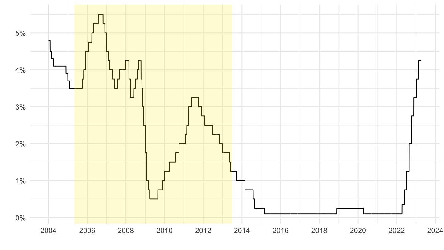
Japan
All
Code
CBPOL_D %>%

  left_join(REF_AREA, by = "REF_AREA") %>%
  filter(REF_AREA %in% c("JP")) %>%
  ggplot(.) + geom_line(aes(x = date, y = value/100)) +
  theme_minimal() + xlab("") + ylab("") +
  scale_x_date(breaks = seq(1940, 2100, 5) %>% paste0("-01-01") %>% as.Date,
               labels = date_format("%Y")) +
  scale_y_continuous(breaks = 0.01*seq(0, 10000, 1),
                labels = percent_format(accuracy = 1)) +
  scale_color_manual(values = viridis(4)[1:3]) +
  theme(legend.position = c(0.8, 0.80),
        legend.title = element_blank())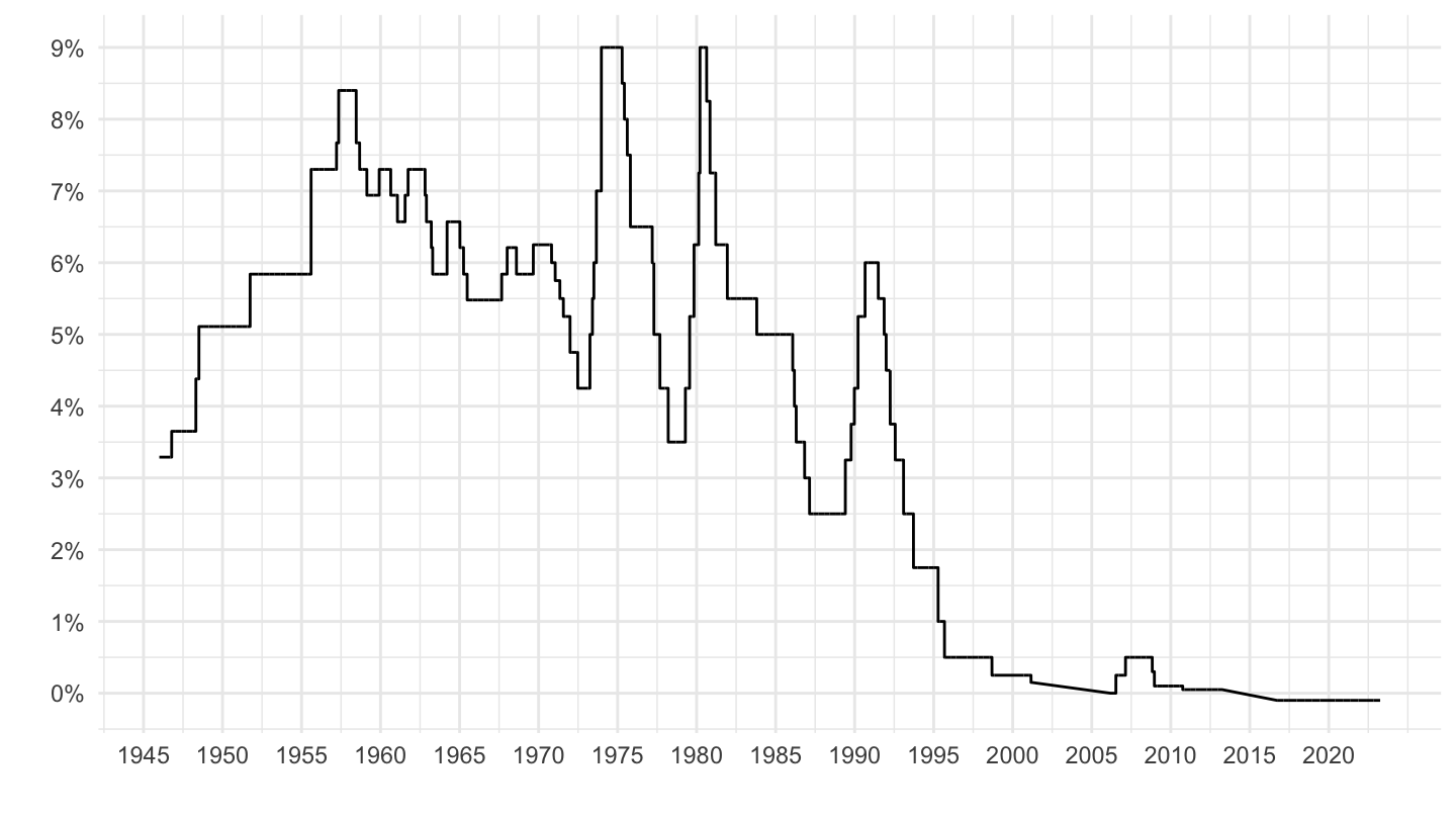
1980-
Code
CBPOL_D %>%

  left_join(REF_AREA, by = "REF_AREA") %>%
  filter(REF_AREA %in% c("JP"),
         date >= as.Date("1980-01-01")) %>%
  ggplot(.) + geom_line(aes(x = date, y = value/100)) +
  theme_minimal() + xlab("") + ylab("") +
  scale_x_date(breaks = seq(1940, 2100, 2) %>% paste0("-01-01") %>% as.Date,
               labels = date_format("%Y")) +
  scale_y_continuous(breaks = 0.01*seq(0, 10000, 0.5),
                labels = percent_format(accuracy = .1)) +
  scale_color_manual(values = viridis(4)[1:3]) +
  theme(legend.position = c(0.8, 0.80),
        legend.title = element_blank())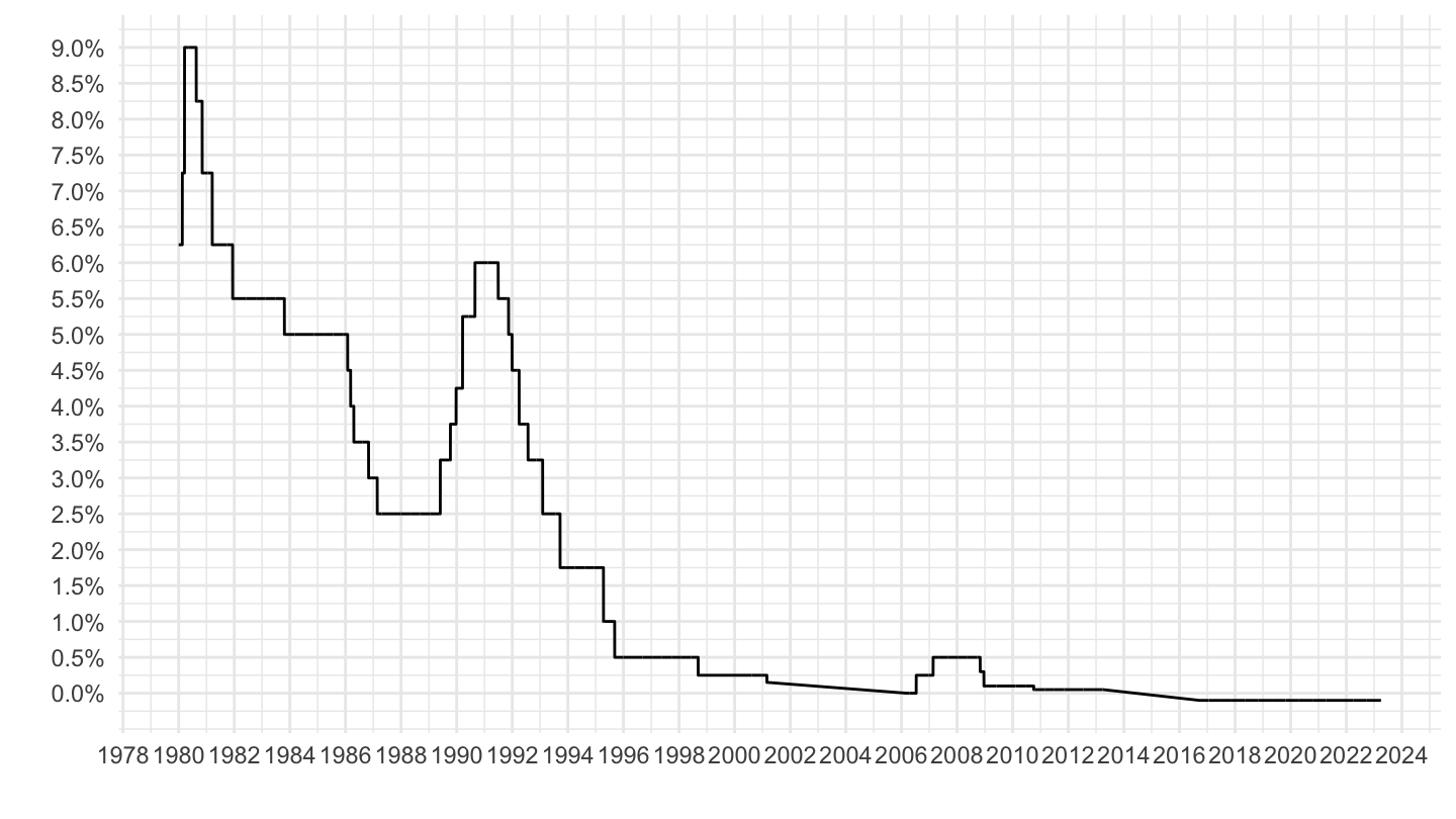
1990-
Code
CBPOL_D %>%

  left_join(REF_AREA, by = "REF_AREA") %>%
  filter(REF_AREA %in% c("JP"),
         date >= as.Date("1990-01-01")) %>%
  ggplot(.) + geom_line(aes(x = date, y = value/100)) +
  theme_minimal() + xlab("") + ylab("") +
  scale_x_date(breaks = seq(1940, 2100, 2) %>% paste0("-01-01") %>% as.Date,
               labels = date_format("%Y")) +
  scale_y_continuous(breaks = 0.01*seq(0, 10000, 0.5),
                labels = percent_format(accuracy = .1)) +
  scale_color_manual(values = viridis(4)[1:3]) +
  theme(legend.position = c(0.8, 0.80),
        legend.title = element_blank())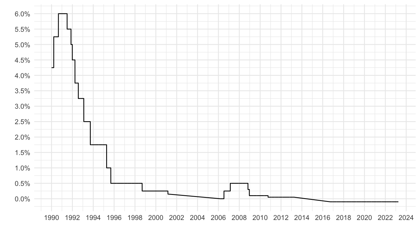
2000-
Code
CBPOL_D %>%

  left_join(REF_AREA, by = "REF_AREA") %>%
  filter(REF_AREA %in% c("JP"),
         date >= as.Date("2000-01-01")) %>%
  ggplot(.) + geom_line(aes(x = date, y = value/100)) +
  theme_minimal() + xlab("") + ylab("") +
  scale_x_date(breaks = seq(1940, 2100, 2) %>% paste0("-01-01") %>% as.Date,
               labels = date_format("%Y")) +
  scale_y_continuous(breaks = 0.01*seq(0, 10000, 0.1),
                labels = percent_format(accuracy = .1)) +
  scale_color_manual(values = viridis(4)[1:3]) +
  theme(legend.position = c(0.8, 0.80),
        legend.title = element_blank())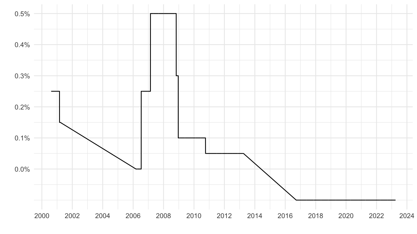
2010-
Code
CBPOL_D %>%

  left_join(REF_AREA, by = "REF_AREA") %>%
  filter(REF_AREA %in% c("JP"),
         date >= as.Date("2010-01-01")) %>%
  ggplot(.) + geom_line(aes(x = date, y = value/100)) +
  theme_minimal() + xlab("") + ylab("") +
  scale_x_date(breaks = seq(1940, 2100, 2) %>% paste0("-01-01") %>% as.Date,
               labels = date_format("%Y")) +
  scale_y_continuous(breaks = 0.01*seq(0, 10000, 0.1),
                labels = percent_format(accuracy = .1)) +
  scale_color_manual(values = viridis(4)[1:3]) +
  theme(legend.position = c(0.8, 0.80),
        legend.title = element_blank())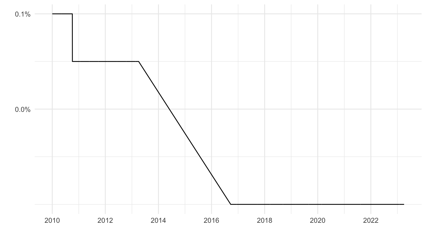
2 Countries
United States, Euro area (1980-)
1999-
English
Code
CBPOL_D %>%

  left_join(REF_AREA, by = "REF_AREA") %>%
  filter(REF_AREA %in% c("US", "XM"),
         date >= as.Date("1999-01-01")) %>%
  mutate(value = value/100,
         OBS_VALUE = value,
         `Reference area` = ifelse(REF_AREA == "XM", "Europe", `Reference area`)) %>%
  ggplot(.) + geom_line(aes(x = date, y = value, color = `Reference area`)) +
  theme_minimal() + xlab("") + ylab("") + add_flags +
  scale_x_date(breaks = seq(1940, 2100, 2) %>% paste0("-01-01") %>% as.Date,
               labels = date_format("%Y")) +
  scale_y_continuous(breaks = 0.01*seq(-5, 30, 1),
                labels = percent_format(accuracy = 1)) +
  scale_color_manual(values = c("#003399", "#B22234")) +
  theme(legend.position = c(0.8, 0.80),
        legend.title = element_blank())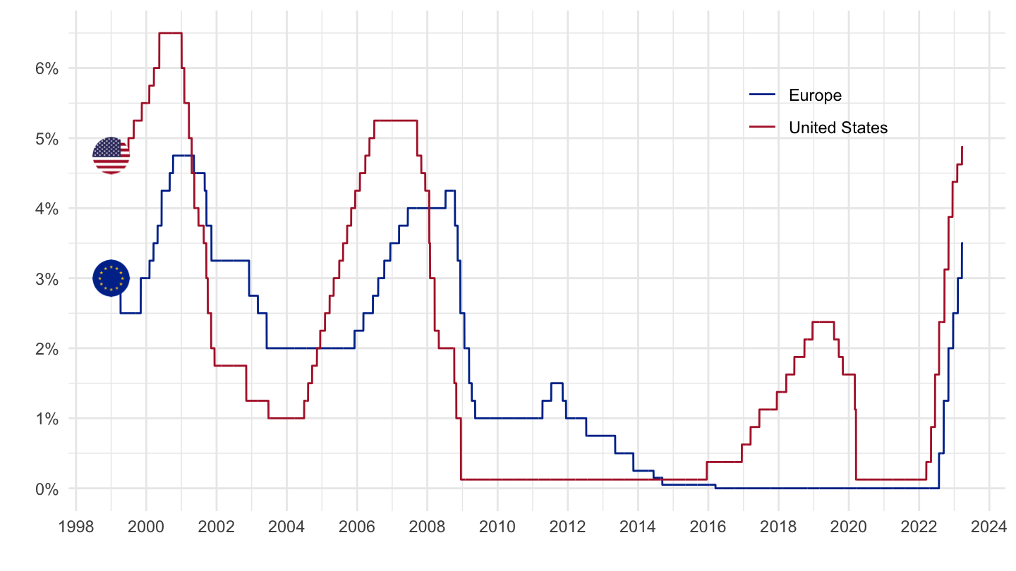
French
Code
plot <- CBPOL_D %>%
  left_join(REF_AREA, by = "REF_AREA") %>%
  filter(REF_AREA %in% c("US", "XM"),
         date >= as.Date("1999-01-01")) %>%
  mutate(value = value/100,
         OBS_VALUE = value,
         `Reference area` = ifelse(REF_AREA == "XM", "Europe", `Reference area`),
         Ref_area2 = ifelse(REF_AREA == "XM", "Zone euro", "États-Unis")) %>%
  ggplot(.) + geom_line(aes(x = date, y = value, color = Ref_area2)) +
  theme_minimal() + xlab("") + ylab("") +
  scale_x_date(breaks = seq(1999, 2100, 2) %>% paste0("-01-01") %>% as.Date,
               labels = date_format("%Y")) +
  scale_y_continuous(breaks = 0.01*seq(-5, 30, 1),
                labels = percent_format(accuracy = 1)) +
  scale_color_manual(values = c( "#B22234", "#003399")) +
  theme(legend.position = c(0.8, 0.80),
        legend.title = element_blank()) +
  geom_rect(data = nber_recessions %>%
              filter(Peak > as.Date("1999-01-01")),
            aes(xmin = Peak, xmax = Trough, ymin = -Inf, ymax = +Inf),
            fill = '#B22234', alpha = 0.1)  +
  geom_rect(data = cepr_recessions %>%
              filter(Peak > as.Date("1999-01-01")),
            aes(xmin = Peak, xmax = Trough, ymin = -Inf, ymax = +Inf),
            fill = '#003399', alpha = 0.1)
plot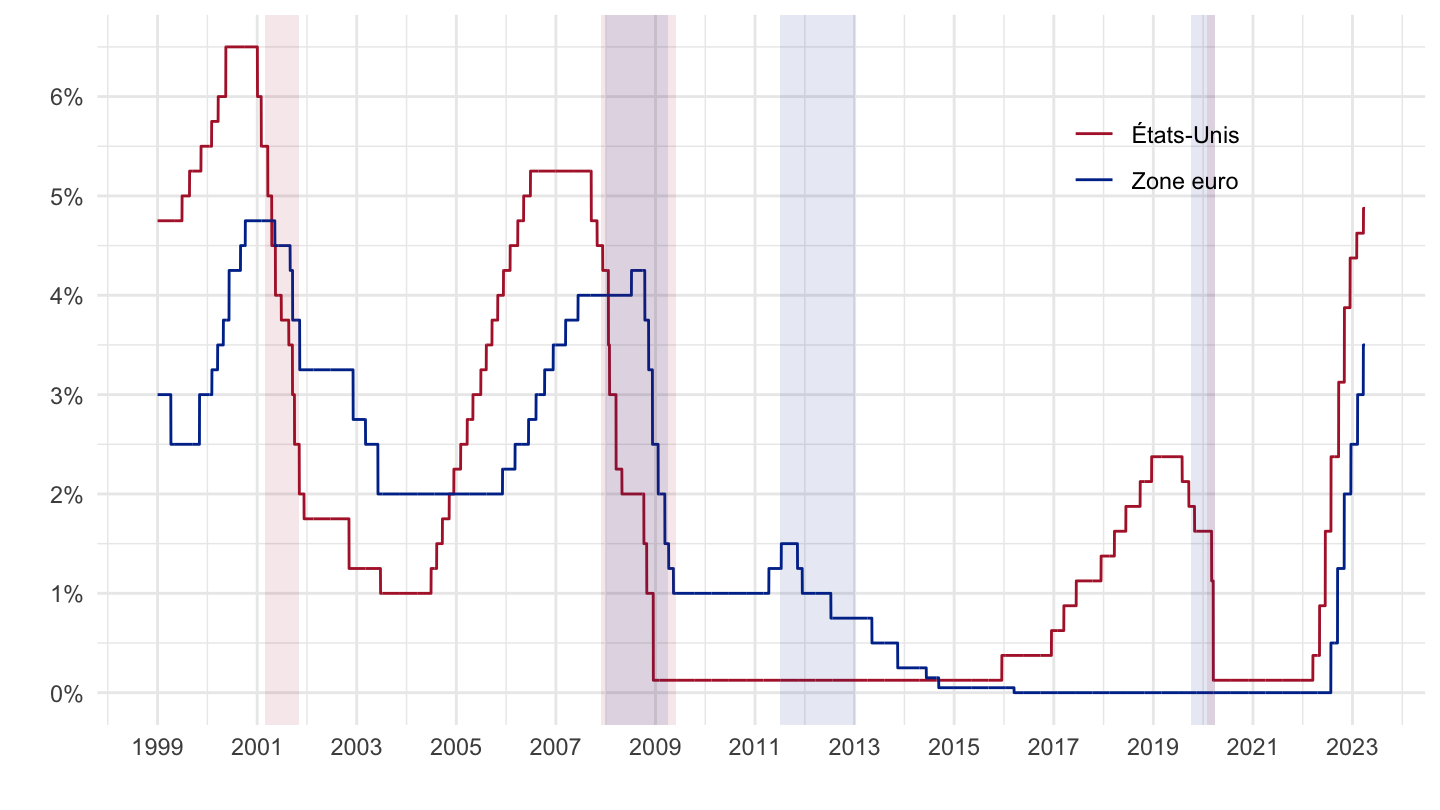
Code
save(plot, file = "CBPOL_D_files/figure-html/US-XM-1999-francais-1.RData")2008-
Code
CBPOL_D %>%

  left_join(REF_AREA, by = "REF_AREA") %>%
  filter(REF_AREA %in% c("US", "XM"),
         date >= as.Date("2008-01-01")) %>%
  mutate(value = value/100,
         OBS_VALUE = value,
         `Reference area` = ifelse(REF_AREA == "XM", "Europe", `Reference area`)) %>%
  arrange(desc(date)) %>%
  left_join(colors, by = c("Reference area" = "country")) %>%
  mutate(color = ifelse(REF_AREA == "XM", color2, color)) %>%
  ggplot(.) + geom_line(aes(x = date, y = value, color = color)) +
  theme_minimal() + xlab("") + ylab("") + add_flags + scale_color_identity() +
  scale_x_date(breaks = seq(1940, 2100, 2) %>% paste0("-01-01") %>% as.Date,
               labels = date_format("%Y")) +
  scale_y_continuous(breaks = 0.01*seq(-5, 30, 1),
                labels = percent_format(accuracy = 1))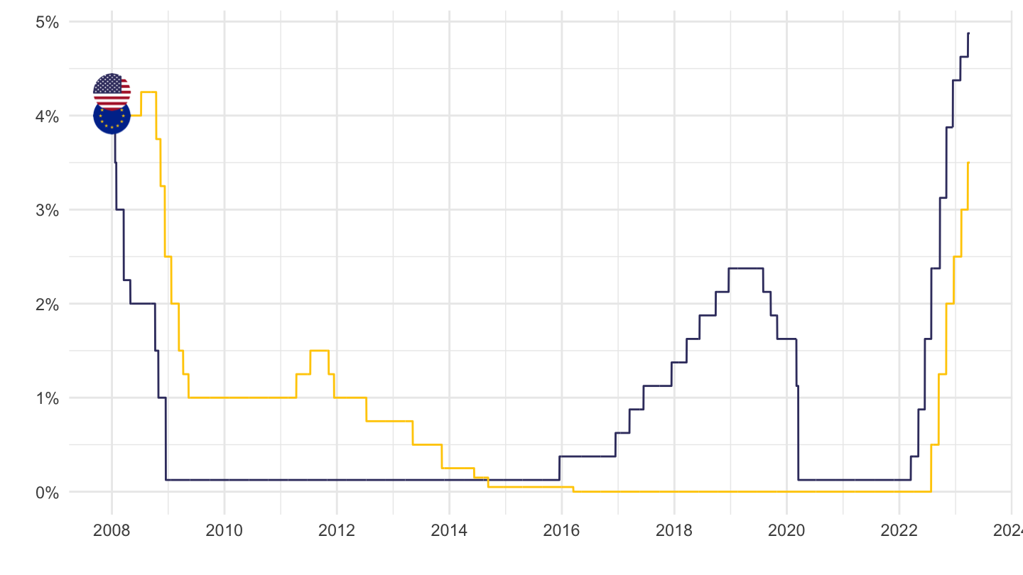
2013-
Code
CBPOL_D %>%

  left_join(REF_AREA, by = "REF_AREA") %>%
  filter(REF_AREA %in% c("US", "XM"),
         date >= as.Date("2013-01-01")) %>%
  mutate(value = value/100,
         OBS_VALUE = value,
         `Reference area` = ifelse(REF_AREA == "XM", "Europe", `Reference area`)) %>%
  arrange(desc(date)) %>%
  left_join(colors, by = c("Reference area" = "country")) %>%
  mutate(color = ifelse(REF_AREA == "XM", color2, color)) %>%
  ggplot(.) + geom_line(aes(x = date, y = value, color = color)) +
  theme_minimal() + xlab("") + ylab("") + add_flags + scale_color_identity() +
  scale_x_date(breaks = seq(1940, 2100, 1) %>% paste0("-01-01") %>% as.Date,
               labels = date_format("%Y")) +
  scale_y_continuous(breaks = 0.01*seq(-5, 30, 1),
                labels = percent_format(accuracy = 1))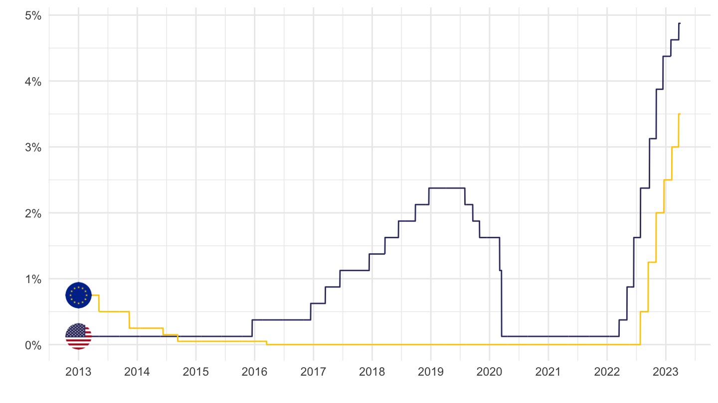
Last 10 years
Code
CBPOL_D %>%

  left_join(REF_AREA, by = "REF_AREA") %>%
  filter(REF_AREA %in% c("US", "XM"),
         date >= Sys.Date() - years(10)) %>%
  mutate(value = value/100,
         OBS_VALUE = value,
         `Reference area` = ifelse(REF_AREA == "XM", "Europe", `Reference area`)) %>%
  arrange(desc(date)) %>%
  left_join(colors, by = c("Reference area" = "country")) %>%
  mutate(color = ifelse(REF_AREA == "XM", color2, color)) %>%
  ggplot(.) + geom_line(aes(x = date, y = value, color = color)) +
  theme_minimal() + xlab("") + ylab("") + add_flags + scale_color_identity() +
  scale_x_date(breaks = seq(1940, 2100, 1) %>% paste0("-01-01") %>% as.Date,
               labels = date_format("%Y")) +
  scale_y_continuous(breaks = 0.01*seq(-5, 30, 1),
                labels = percent_format(accuracy = 1))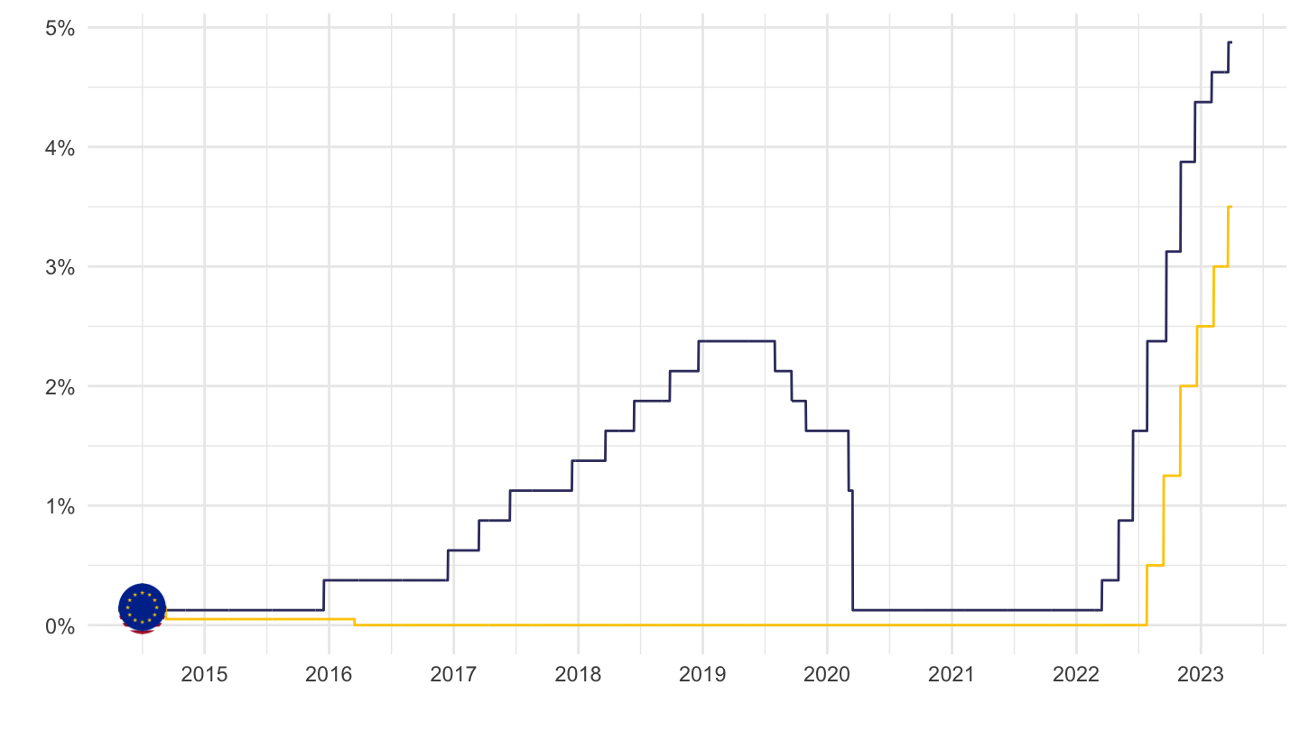
2022-
Dates
Code
dates_ecb <- CBPOL_D %>%
  filter(REF_AREA == "XM",
         date >= as.Date("2022-01-01")) %>%
  mutate(value = value-lag(value), OBS_VALUE = value) %>%
  filter(value != 0) %>%
  pull(date)
dates_fed <- CBPOL_D %>%
  filter(REF_AREA == "US",
         date >= as.Date("2022-01-01")) %>%
  mutate(value = value-lag(value), OBS_VALUE = value) %>%
  filter(value != 0) %>%
  pull(date)
CBPOL_D %>%
  left_join(REF_AREA, by = "REF_AREA") %>%
  filter(REF_AREA %in% c("US", "XM"),
         date >= as.Date("2022-01-01")) %>%
  mutate(value = value/100,
         OBS_VALUE = value,
         `Reference area` = ifelse(REF_AREA == "XM", "Euro area, Main Refinancing Operations", "US, Fed Funds rate")) %>%
  arrange(desc(date)) %>%
  ggplot(.) + geom_line(aes(x = date, y = value, color = `Reference area`)) +
  theme_minimal() + xlab("") + ylab("") + scale_color_identity() +
  scale_color_manual(values = c("#003399", "#B22234")) +
  scale_x_date(breaks = c(dates_ecb),
               labels = date_format("%d %b %Y"),
               sec.axis = dup_axis(breaks = dates_fed)) +
  scale_y_continuous(breaks = 0.01*seq(-5, 30, 1),
                labels = percent_format(accuracy = 1),
                limits = c(0, 0.06)) +
  theme(legend.position = c(0.25, 0.85),
        legend.title = element_blank(),
        axis.text.x.top = element_text(angle = 45, hjust = 0, colour = "#B22234"),
        axis.text.x.bottom = element_text(angle = 45, hjust = 1, colour = "#003399"))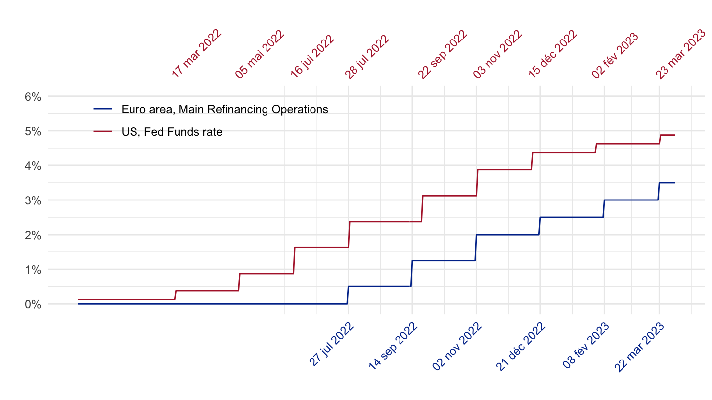
Dates
Code
dates_ecb <- CBPOL_D %>%
  filter(REF_AREA == "XM",
         date >= as.Date("2022-01-01")) %>%
  mutate(value = value-lag(value), OBS_VALUE = value) %>%
  filter(value != 0) %>%
  pull(date)
dates_fed <- CBPOL_D %>%
  filter(REF_AREA == "US",
         date >= as.Date("2022-01-01")) %>%
  mutate(value = value-lag(value), OBS_VALUE = value) %>%
  filter(value != 0) %>%
  pull(date)
CBPOL_D %>%
  left_join(REF_AREA, by = "REF_AREA") %>%
  filter(REF_AREA %in% c("US", "XM"),
         date >= as.Date("2022-01-01")) %>%
  mutate(value = value/100,
         OBS_VALUE = value,
         `Reference area` = ifelse(REF_AREA == "XM", "Euro area, Main Refinancing Operations",
                           "US, Fed Funds rate")) %>%
  arrange(desc(date)) %>%
  ggplot(.) + geom_line(aes(x = date, y = value, color = `Reference area`)) +
  theme_minimal() + xlab("") + ylab("") + scale_color_identity() +
  scale_color_manual(values = c("#003399", "#B22234")) +
  scale_x_date(breaks = c(dates_ecb),
               labels = date_format("%d %b %Y"),
               sec.axis = dup_axis(breaks = dates_fed)) +
  scale_y_continuous(breaks = 0.01*seq(-5, 30, 1),
                labels = percent_format(accuracy = 1),
                limits = c(0, 0.06)) +
  theme(legend.position = "top",
        legend.title = element_blank(),
        axis.text.x.top = element_text(angle = 45, hjust = 0, colour = "#B22234"),
        axis.text.x.bottom = element_text(angle = 45, hjust = 1, colour = "#003399")) +
  sapply(dates_fed, function(x) geom_vline(xintercept = x, linetype = "dotted", colour = "#B22234")) +
  sapply(dates_ecb, function(x) geom_vline(xintercept = x, linetype = "dotted", colour = "#003399"))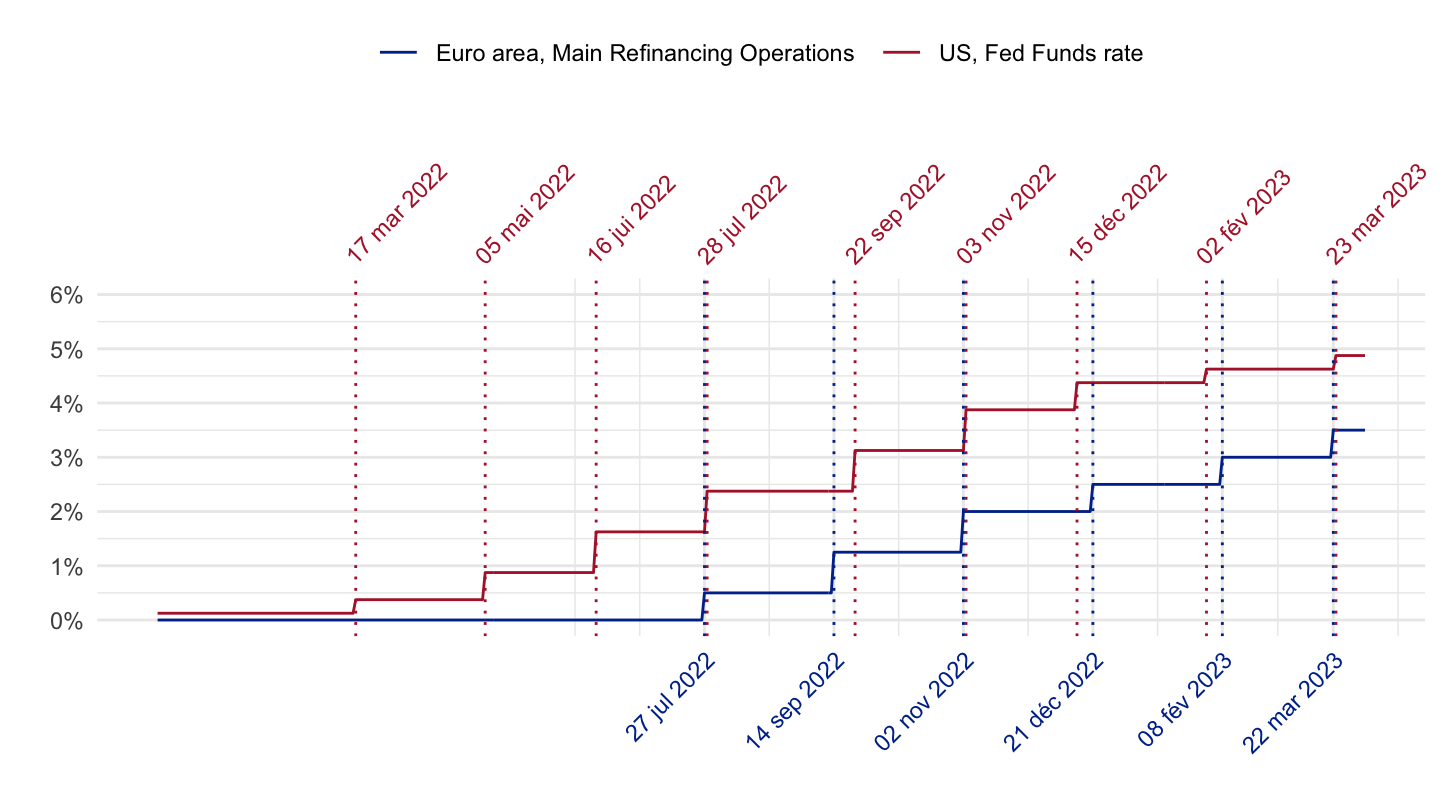
Dates, deposit
English
Code
Sys.setlocale("LC_TIME", "en_CA.UTF-8")# [1] "en_CA.UTF-8"Code
dates_ecb <- CBPOL_D %>%
  filter(REF_AREA == "XM",
         date >= as.Date("2022-01-01")) %>%
  mutate(value = value-lag(value), OBS_VALUE = value) %>%
  filter(value != 0) %>%
  pull(date)
dates_fed <- CBPOL_D %>%
  filter(REF_AREA == "US",
         date >= as.Date("2022-01-01")) %>%
  mutate(value = value-lag(value), OBS_VALUE = value) %>%
  filter(value != 0) %>%
  pull(date)

CBPOL_D %>%
  left_join(REF_AREA, by = "REF_AREA") %>%
  filter(REF_AREA %in% c("US", "XM"),
         date >= as.Date("2022-01-01")) %>%
  mutate(value = value/100,
         OBS_VALUE = value,
         `Reference area` = ifelse(REF_AREA == "XM", "Euro area, Deposit facility rate",
                           "US, Federal funds rate (midpoint)")) %>%
  arrange(desc(date)) %>%
  mutate(value = ifelse(REF_AREA == "XM", value - 0.005, value),
         OBS_VALUE = value) %>%
  ggplot(.) + geom_line(aes(x = date, y = value, color = `Reference area`)) +
  theme_minimal() + xlab("") + ylab("") + scale_color_identity() +
  scale_color_manual(values = c("#003399", "#B22234")) +
  scale_x_date(breaks = c(dates_ecb),
               labels = date_format("%d %b %Y"),
               sec.axis = dup_axis(breaks = dates_fed)) +
  scale_y_continuous(breaks = 0.01*seq(-5, 30, 1),
                labels = percent_format(accuracy = 1),
                limits = c(-0.01, 0.06)) +
  theme(legend.position = "top",
        legend.title = element_blank(),
        axis.text.x.top = element_text(angle = 45, hjust = 0, colour = "#B22234"),
        axis.text.x.bottom = element_text(angle = 45, hjust = 1, colour = "#003399")) +
  sapply(dates_fed, function(x) geom_vline(xintercept = x, linetype = "dotted", colour = "#B22234")) +
  sapply(dates_ecb, function(x) geom_vline(xintercept = x, linetype = "dotted", colour = "#003399"))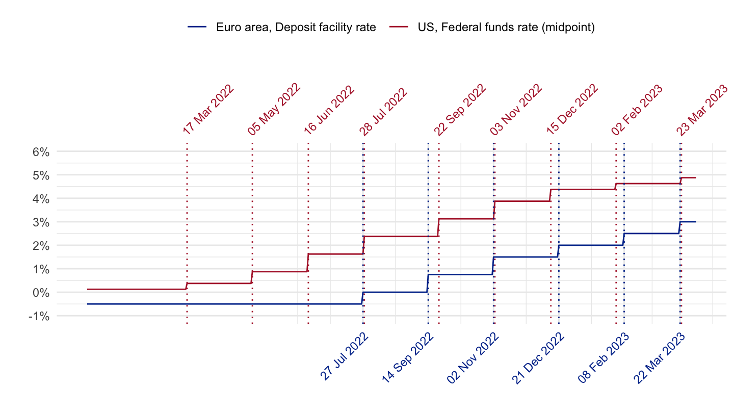
French
Code
Sys.setlocale("LC_TIME", "fr_CA.UTF-8")# [1] "fr_CA.UTF-8"Code
dates_ecb <- CBPOL_D %>%
  filter(REF_AREA == "XM",
         date >= as.Date("2022-01-01")) %>%
  mutate(value = value-lag(value), OBS_VALUE = value) %>%
  filter(value != 0) %>%
  pull(date)
dates_fed <- CBPOL_D %>%
  filter(REF_AREA == "US",
         date >= as.Date("2022-01-01")) %>%
  mutate(value = value-lag(value), OBS_VALUE = value) %>%
  filter(value != 0) %>%
  pull(date)

dates_ecb <- c(dates_ecb, as.Date("2024-09-12"))

CBPOL_D %>%
  left_join(REF_AREA, by = "REF_AREA") %>%
  filter(REF_AREA %in% c("US", "XM"),
         date >= as.Date("2022-01-01")) %>%
  mutate(value = value/100,
         OBS_VALUE = value,
         `Reference area` = ifelse(REF_AREA == "XM",
                           "Zone euro, Taux de la facilité de dépôt",
                           "États-Unis, Taux des Feds Funds"),
         `Reference area` = factor(`Reference area`, levels = c("Zone euro, Taux de la facilité de dépôt",
                           "États-Unis, Taux des Feds Funds"))) %>%
  arrange(desc(date)) %>%
  mutate(value = ifelse(REF_AREA == "XM", value - 0.005, value),
         OBS_VALUE = value) %>%
  ggplot(.) + geom_line(aes(x = date, y = value, color = `Reference area`)) +
  theme_minimal() + xlab("") + ylab("") + scale_color_identity() +
  scale_color_manual(values = c("#003399", "#B22234")) +
  scale_x_date(breaks = c(dates_ecb),
               labels = date_format("%d %b %Y"),
               sec.axis = dup_axis(breaks = dates_fed)) +
  scale_y_continuous(breaks = 0.01*seq(-5, 30, 1),
                labels = percent_format(accuracy = 1),
                limits = c(-0.01, 0.06)) +
  theme(legend.position = "top",
        legend.title = element_blank(),
        axis.text.x.top = element_text(angle = 45, hjust = 0, colour = "#B22234"),
        axis.text.x.bottom = element_text(angle = 45, hjust = 1, colour = "#003399")) +
  sapply(dates_fed, function(x) geom_vline(xintercept = x, linetype = "dotted", colour = "#B22234")) +
  sapply(dates_ecb, function(x) geom_vline(xintercept = x, linetype = "dotted", colour = "#003399"))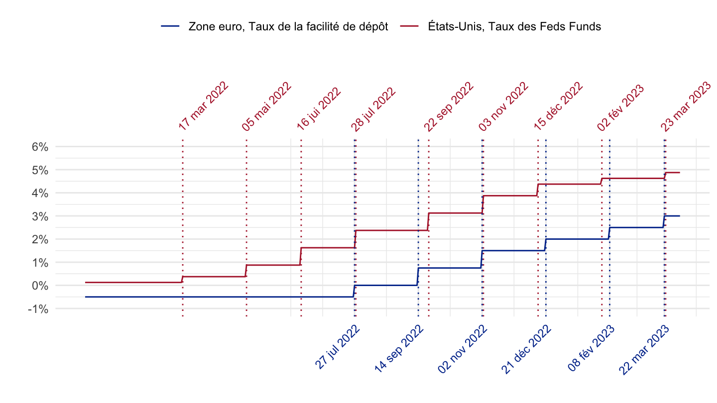
Code
Sys.setlocale("LC_TIME", "en_CA.UTF-8")# [1] "en_CA.UTF-8"2007-2014
All
Code
CBPOL_D %>%
  left_join(REF_AREA, by = "REF_AREA") %>%
  filter(REF_AREA %in% c("US", "XM"),
         date >= as.Date("2007-01-01"),
         date <= as.Date("2014-12-31")) %>%
  mutate(value = value/100,
         OBS_VALUE = value,
         `Reference area` = ifelse(REF_AREA == "XM", "Europe", `Reference area`)) %>%
  ggplot(.) + geom_line(aes(x = date, y = value, color = `Reference area`)) +
  theme_minimal() + xlab("") + ylab("") + add_flags +
  scale_x_date(breaks = seq(1940, 2100, 1) %>% paste0("-01-01") %>% as.Date,
               labels = date_format("%Y")) +
  scale_y_continuous(breaks = 0.01*seq(-5, 30, .5),
                labels = percent_format(accuracy = .1)) +
  scale_color_manual(values = c("#003399", "#B22234")) +
  theme(legend.position = c(0.8, 0.80),
        legend.title = element_blank())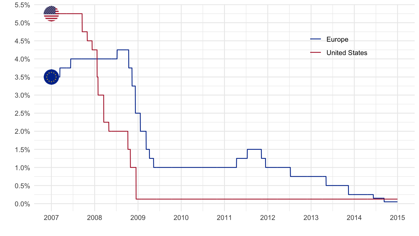
Dates
Code
dates_ecb <- CBPOL_D %>%
  filter(REF_AREA == "XM",
         date >= as.Date("2007-01-01"),
         date <= as.Date("2015-01-01")) %>%
  mutate(value = value-lag(value), OBS_VALUE = value) %>%
  filter(value != 0) %>%
  pull(date)
dates_fed <- CBPOL_D %>%
  filter(REF_AREA == "US",
         date >= as.Date("2007-01-01"),
         date <= as.Date("2015-01-01")) %>%
  mutate(value = value-lag(value), OBS_VALUE = value) %>%
  filter(value != 0) %>%
  pull(date)
CBPOL_D %>%
  left_join(REF_AREA, by = "REF_AREA") %>%
  filter(REF_AREA %in% c("US", "XM"),
         date >= as.Date("2007-01-01"),
         date <= as.Date("2015-01-01")) %>%
  mutate(value = value/100,
         OBS_VALUE = value,
         `Reference area` = ifelse(REF_AREA == "XM", "Euro area, Main Refinancing Operations", "US, Fed Funds rate")) %>%
  arrange(desc(date)) %>%
  ggplot(.) + geom_line(aes(x = date, y = value, color = `Reference area`)) +
  theme_minimal() + xlab("") + ylab("") + scale_color_identity() +
  scale_color_manual(values = c("#003399", "#B22234")) +
  scale_x_date(breaks = c(dates_ecb),
               labels = date_format("%d %b %Y"),
               sec.axis = dup_axis(breaks = dates_fed)) +
  scale_y_continuous(breaks = 0.01*seq(-5, 30, 0.25),
                labels = percent_format(accuracy = .01)) +
  theme(legend.position = c(0.65, 0.85),
        legend.title = element_blank(),
        axis.text.x.top = element_text(angle = 45, hjust = 0, colour = "#B22234"),
        axis.text.x.bottom = element_text(angle = 45, hjust = 1, colour = "#003399"))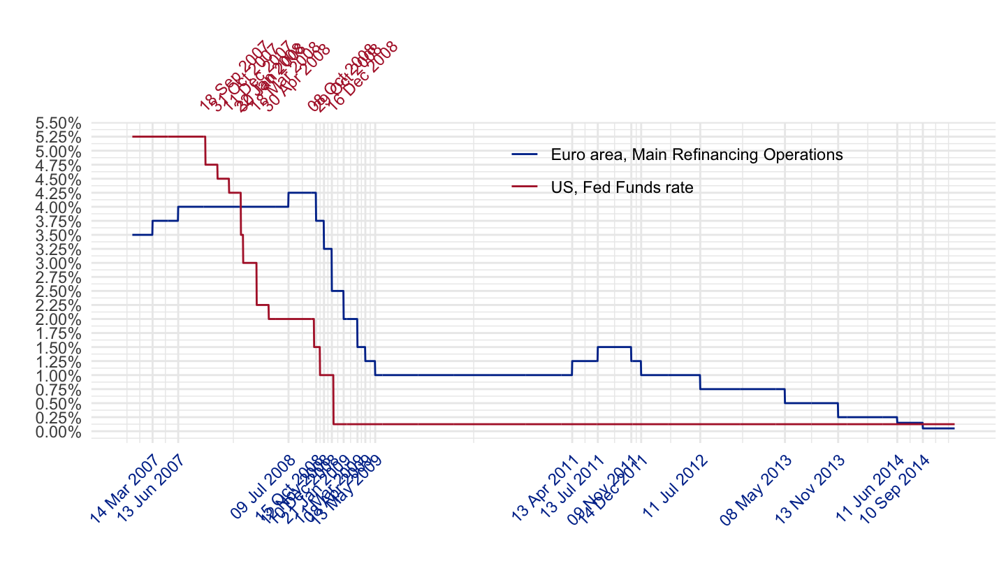
2009-2014
All
Code
CBPOL_D %>%
  left_join(REF_AREA, by = "REF_AREA") %>%
  filter(REF_AREA %in% c("US", "XM"),
         date >= as.Date("2009-01-01"),
         date <= as.Date("2014-12-31")) %>%
  mutate(value = value/100,
         OBS_VALUE = value,
         `Reference area` = ifelse(REF_AREA == "XM", "Europe", `Reference area`)) %>%
  ggplot(.) + geom_line(aes(x = date, y = value, color = `Reference area`)) +
  theme_minimal() + xlab("") + ylab("") + add_flags +
  scale_x_date(breaks = seq(1940, 2100, 1) %>% paste0("-01-01") %>% as.Date,
               labels = date_format("%Y")) +
  scale_y_continuous(breaks = 0.01*seq(-5, 30, .5),
                labels = percent_format(accuracy = .1)) +
  scale_color_manual(values = c("#003399", "#B22234")) +
  theme(legend.position = c(0.8, 0.80),
        legend.title = element_blank())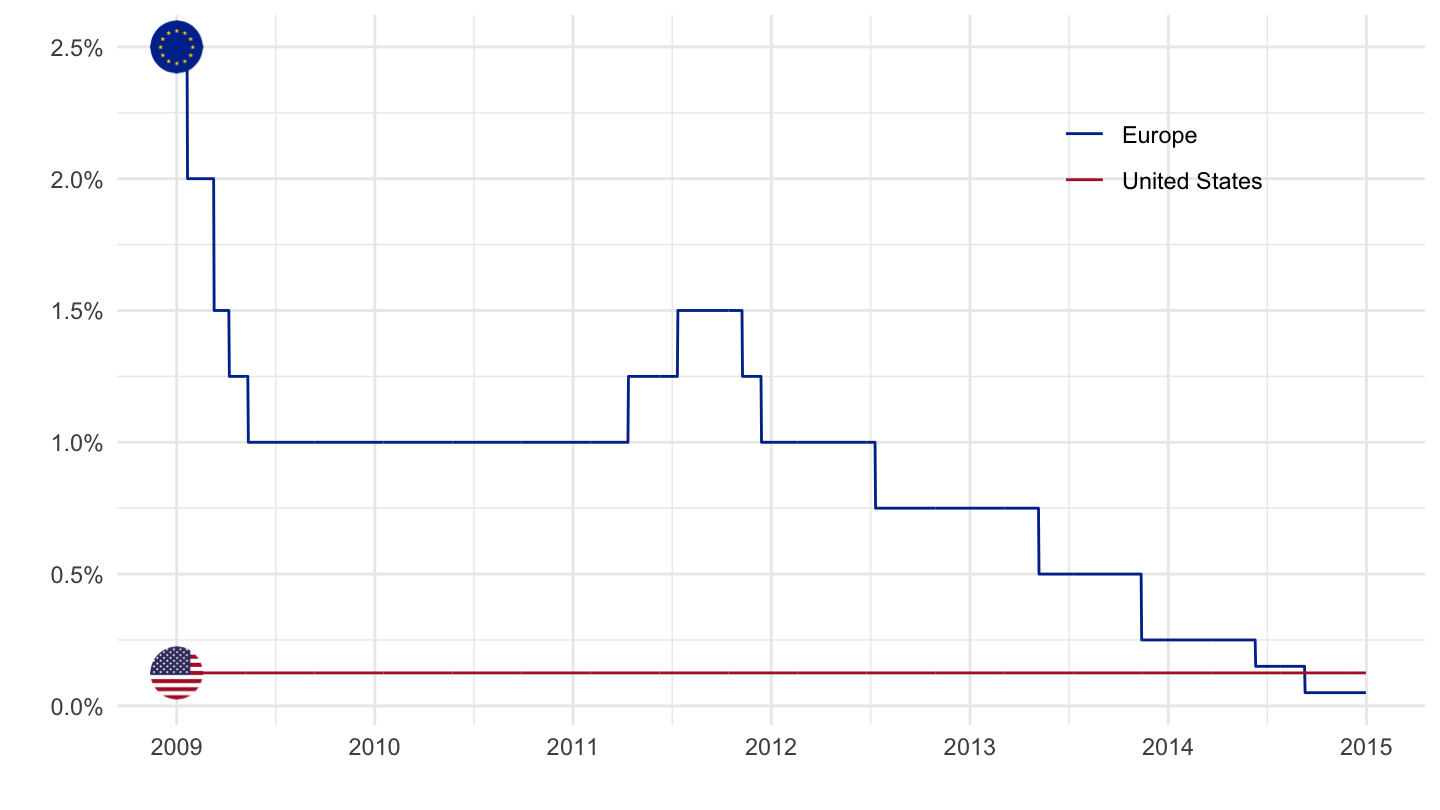
Dates
Code
dates_ecb <- CBPOL_D %>%
  filter(REF_AREA == "XM",
         date >= as.Date("2009-01-01"),
         date <= as.Date("2015-01-01")) %>%
  mutate(value = value-lag(value), OBS_VALUE = value) %>%
  filter(value != 0) %>%
  pull(date)
dates_fed <- CBPOL_D %>%
  filter(REF_AREA == "US",
         date >= as.Date("2009-01-01"),
         date <= as.Date("2015-01-01")) %>%
  mutate(value = value-lag(value), OBS_VALUE = value) %>%
  filter(value != 0) %>%
  pull(date)
CBPOL_D %>%
  left_join(REF_AREA, by = "REF_AREA") %>%
  filter(REF_AREA %in% c("US", "XM"),
         date >= as.Date("2009-01-01"),
         date <= as.Date("2015-01-01")) %>%
  mutate(value = value/100,
         OBS_VALUE = value,
         `Reference area` = ifelse(REF_AREA == "XM", "Euro area, Main Refinancing Operations", "US, Fed Funds rate")) %>%
  arrange(desc(date)) %>%
  ggplot(.) + geom_line(aes(x = date, y = value, color = `Reference area`)) +
  theme_minimal() + xlab("") + ylab("") + scale_color_identity() +
  scale_color_manual(values = c("#003399", "#B22234")) +
  scale_x_date(breaks = c(dates_ecb),
               labels = date_format("%d %b %Y"),
               sec.axis = dup_axis(breaks = dates_fed)) +
  scale_y_continuous(breaks = 0.01*seq(-5, 30, 0.25),
                labels = percent_format(accuracy = .01),
                limits = c(0, 0.015)) +
  theme(legend.position = c(0.65, 0.85),
        legend.title = element_blank(),
        axis.text.x.top = element_text(angle = 45, hjust = 0, colour = "#B22234"),
        axis.text.x.bottom = element_text(angle = 45, hjust = 1, colour = "#003399"))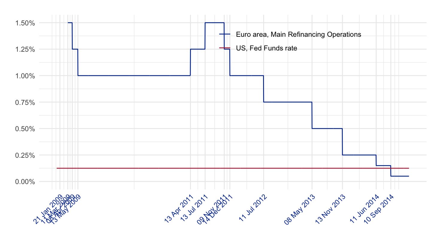
2011-2014
Dates
Code
dates_ecb <- CBPOL_D %>%
  filter(REF_AREA == "XM",
         date >= as.Date("2011-01-01"),
         date <= as.Date("2015-01-01")) %>%
  mutate(value = value-lag(value), OBS_VALUE = value) %>%
  filter(value != 0) %>%
  pull(date)
dates_fed <- CBPOL_D %>%
  filter(REF_AREA == "US",
         date >= as.Date("2011-01-01"),
         date <= as.Date("2015-01-01")) %>%
  mutate(value = value-lag(value), OBS_VALUE = value) %>%
  filter(value != 0) %>%
  pull(date)
CBPOL_D %>%
  left_join(REF_AREA, by = "REF_AREA") %>%
  filter(REF_AREA %in% c("US", "XM"),
         date >= as.Date("2011-01-01"),
         date <= as.Date("2015-01-01")) %>%
  mutate(value = value/100,
         OBS_VALUE = value,
         `Reference area` = ifelse(REF_AREA == "XM", "Euro area, Main Refinancing Operations", "US, Fed Funds rate")) %>%
  arrange(desc(date)) %>%
  ggplot(.) + geom_line(aes(x = date, y = value, color = `Reference area`)) +
  theme_minimal() + xlab("") + ylab("") + scale_color_identity() +
  scale_color_manual(values = c("#003399", "#B22234")) +
  scale_x_date(breaks = c(dates_ecb),
               labels = date_format("%d %b %Y"),
               sec.axis = dup_axis(breaks = dates_fed)) +
  scale_y_continuous(breaks = 0.01*seq(-5, 30, 0.25),
                labels = percent_format(accuracy = .01),
                limits = c(0, 0.015)) +
  theme(legend.position = c(0.65, 0.85),
        legend.title = element_blank(),
        axis.text.x.top = element_text(angle = 45, hjust = 0, colour = "#B22234"),
        axis.text.x.bottom = element_text(angle = 45, hjust = 1, colour = "#003399"))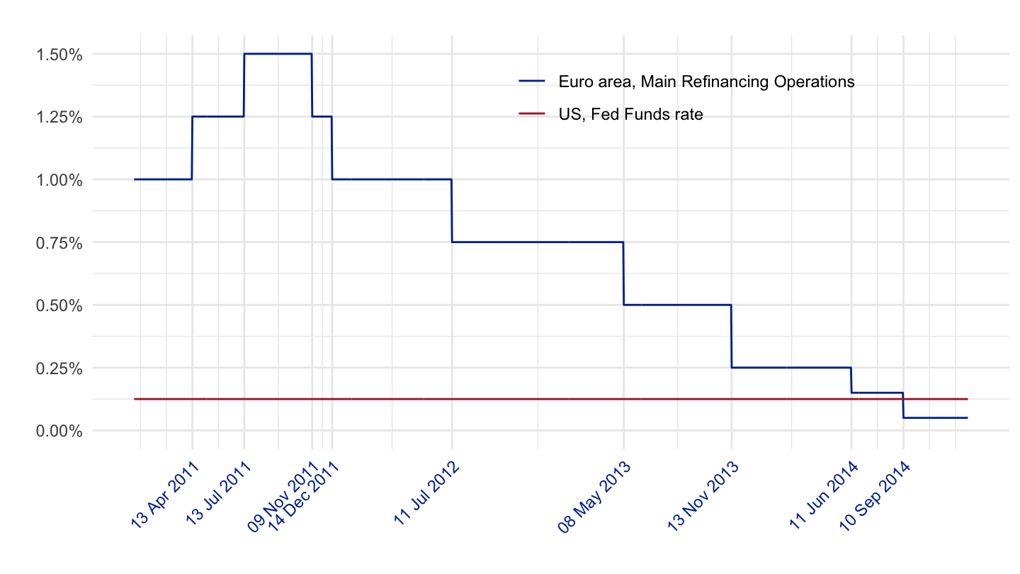
All
Code
CBPOL_D %>%

  left_join(REF_AREA, by = "REF_AREA") %>%
  filter(REF_AREA %in% c("US", "XM")) %>%
  mutate(value = value/100, OBS_VALUE = value) %>%
  ggplot(.) + geom_line(aes(x = date, y = value, color = `Reference area`)) +
  geom_image(data = . %>%
               filter(date == as.Date("2007-01-02")) %>%
               mutate(image = paste0("../../icon/flag/", str_to_lower(gsub(" ", "-", `Reference area`)), ".png")),
             aes(x = date, y = value, image = image), asp = 1.5) +
  theme_minimal() + xlab("") + ylab("") +
  scale_x_date(breaks = seq(1940, 2100, 2) %>% paste0("-01-01") %>% as.Date,
               labels = date_format("%Y")) +
  scale_y_continuous(breaks = 0.01*seq(-5, 30, 1),
                labels = percent_format(accuracy = 1)) +
  scale_color_manual(values = c("#003399", "#B22234")) +
  theme(legend.position = c(0.8, 0.80),
        legend.title = element_blank())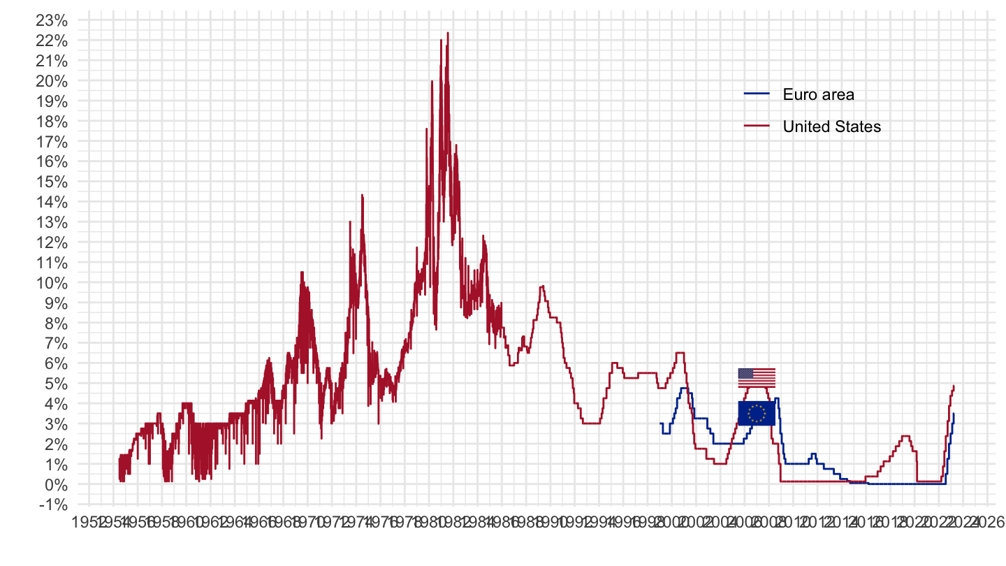
United States, Hong Kong
All
Code
CBPOL_D %>%

  left_join(REF_AREA, by = "REF_AREA") %>%
  filter(REF_AREA %in% c("US", "HK")) %>%
  ggplot(.) + geom_line(aes(x = date, y = value/100, color = `Reference area`)) +
  theme_minimal() + xlab("") + ylab("") +
  scale_x_date(breaks = seq(1940, 2100, 2) %>% paste0("-01-01") %>% as.Date,
               labels = date_format("%Y")) +
  scale_y_continuous(breaks = 0.01*seq(-5, 30, 1),
                labels = percent_format(accuracy = 1)) +
  scale_color_manual(values = c("#DE2408", "#3C3B6E")) +
  theme(legend.position = c(0.8, 0.80),
        legend.title = element_blank())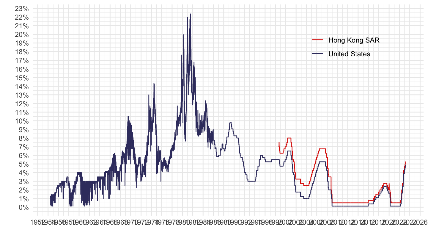
1999-
Code
CBPOL_D %>%

  left_join(REF_AREA, by = "REF_AREA") %>%
  filter(REF_AREA %in% c("US", "HK"),
         date >= as.Date("1999-01-01")) %>%
  mutate(`Reference area` = ifelse(REF_AREA == "HK", "Hong Kong", `Reference area`)) %>%
  mutate(value = value/100, OBS_VALUE = value) %>%
  ggplot(.) + geom_line(aes(x = date, y = value, color = `Reference area`)) +
  add_flags + theme_minimal() + xlab("") + ylab("") +
  scale_x_date(breaks = seq(1940, 2100, 2) %>% paste0("-01-01") %>% as.Date,
               labels = date_format("%Y")) +
  scale_y_continuous(breaks = 0.01*seq(-5, 30, 1),
                labels = percent_format(accuracy = 1)) +
  scale_color_manual(values = c("#DE2408", "#3C3B6E")) +
  theme(legend.position = c(0.8, 0.80),
        legend.title = element_blank())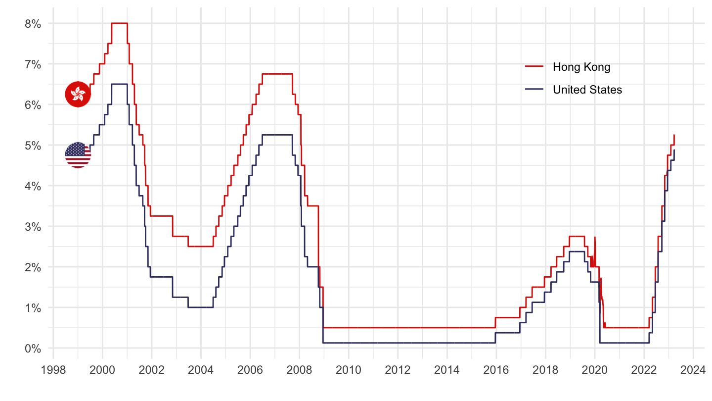
2009-2014
Code
CBPOL_D %>%

  left_join(REF_AREA, by = "REF_AREA") %>%
  filter(REF_AREA %in% c("US", "HK"),
         date >= as.Date("2009-01-01"),
         date <= as.Date("2014-12-31")) %>%
  mutate(`Reference area` = ifelse(REF_AREA == "HK", "Hong Kong", `Reference area`)) %>%
  mutate(value = value/100, OBS_VALUE = value) %>%
  ggplot(.) + geom_line(aes(x = date, y = value, color = `Reference area`)) +
  geom_image(data = . %>%
               filter(date == as.Date("2012-01-04")) %>%
               mutate(image = paste0("../../icon/flag/", str_to_lower(gsub(" ", "-", `Reference area`)), ".png")),
             aes(x = date, y = value, image = image), asp = 1.5) +
  theme_minimal() + xlab("") + ylab("") +
  scale_x_date(breaks = seq(1940, 2100, 1) %>% paste0("-01-01") %>% as.Date,
               labels = date_format("%Y")) +
  scale_y_continuous(breaks = 0.01*seq(-5, 30, .5),
                labels = percent_format(accuracy = .1)) +
  scale_color_manual(values = c("#DE2408", "#3C3B6E")) +
  theme(legend.position = c(0.8, 0.80),
        legend.title = element_blank())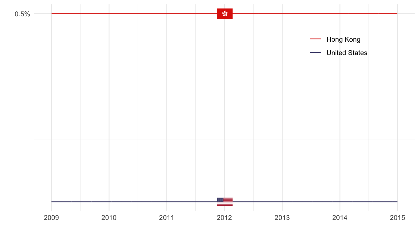
3 Countries
United States, Japan, Euro area
1980-
Code
CBPOL_D %>%

  left_join(REF_AREA, by = "REF_AREA") %>%
  filter(REF_AREA %in% c("US", "JP", "XM"),
         date >= as.Date("1980-01-01")) %>%
  mutate(`Reference area` = ifelse(REF_AREA == "XM", "Europe", `Reference area`)) %>%
  left_join(colors, by = c("Reference area" = "country")) %>%
  mutate(value = value/100, OBS_VALUE = value) %>%
  ggplot(.) + theme_minimal() + xlab("") + ylab("Policy Rates (%)") +
  geom_line(aes(x = date, y = value, color = color)) +
  scale_color_identity() + add_flags +
  scale_x_date(breaks = seq(1940, 2100, 5) %>% paste0("-01-01") %>% as.Date,
               labels = date_format("%Y")) +
  scale_y_continuous(breaks = 0.01*seq(-5, 30, 1),
                labels = percent_format(accuracy = 1)) +
  theme(legend.position = c(0.8, 0.80),
        legend.title = element_blank())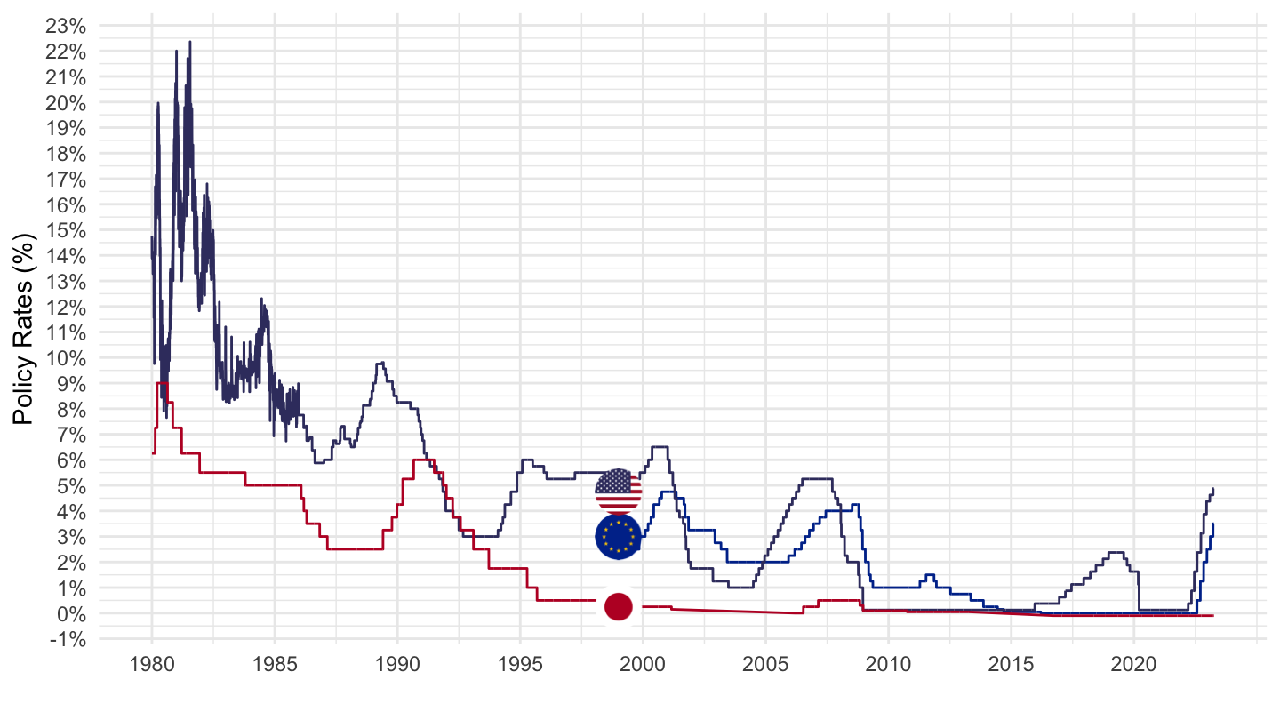
1985-
Code
CBPOL_D %>%

  left_join(REF_AREA, by = "REF_AREA") %>%
  filter(REF_AREA %in% c("US", "JP", "XM"),
         date >= as.Date("1985-01-01")) %>%
  mutate(`Reference area` = ifelse(REF_AREA == "XM", "Europe", `Reference area`)) %>%
  left_join(colors, by = c("Reference area" = "country")) %>%
  mutate(value = value/100, OBS_VALUE = value) %>%
  ggplot(.) + theme_minimal() + xlab("") + ylab("Policy Rates (%)") +
  geom_line(aes(x = date, y = value, color = color)) +
  scale_color_identity() + add_flags +
  scale_x_date(breaks = seq(1940, 2100, 5) %>% paste0("-01-01") %>% as.Date,
               labels = date_format("%Y")) +
  scale_y_continuous(breaks = 0.01*seq(-5, 30, 1),
                labels = percent_format(accuracy = 1)) +
  theme(legend.position = c(0.8, 0.80),
        legend.title = element_blank())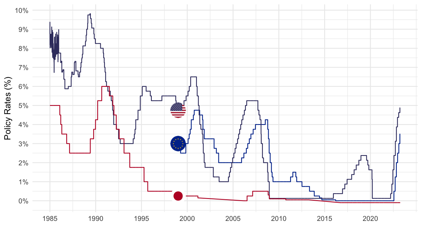
2009-
Code
CBPOL_D %>%

  left_join(REF_AREA, by = "REF_AREA") %>%
  filter(REF_AREA %in% c("US", "JP", "XM"),
         date >= as.Date("2009-01-01")) %>%
  mutate(`Reference area` = ifelse(REF_AREA == "XM", "Europe", `Reference area`),
         value = value/100, OBS_VALUE = value) %>%
  left_join(colors, by = c("Reference area" = "country")) %>%
  ggplot(.) + theme_minimal() + xlab("") + ylab("Policy Rates (%)") +
  geom_line(aes(x = date, y = value, color = color)) +
  scale_color_identity() + add_flags +
  scale_x_date(breaks = seq(1940, 2100, 2) %>% paste0("-01-01") %>% as.Date,
               labels = date_format("%Y")) +
  scale_y_continuous(breaks = 0.01*seq(-5, 30, 1),
                labels = percent_format(accuracy = 1)) +
  theme(legend.position = c(0.8, 0.80),
        legend.title = element_blank())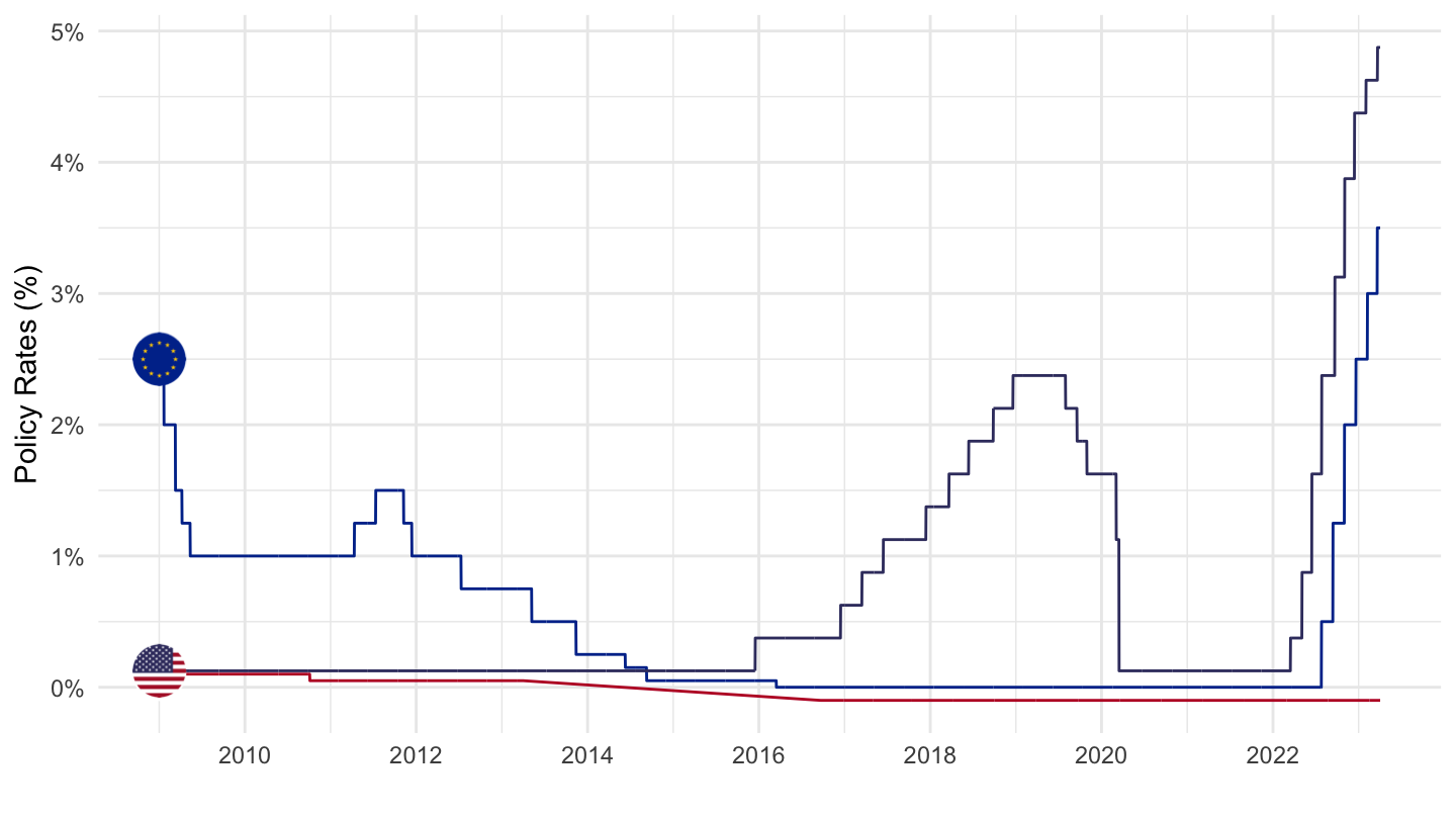
2000-
Code
CBPOL_D %>%

  left_join(REF_AREA, by = "REF_AREA") %>%
  filter(REF_AREA %in% c("US", "JP", "XM"),
         date >= as.Date("2000-01-01")) %>%
  mutate(`Reference area` = ifelse(REF_AREA == "XM", "Europe", `Reference area`)) %>%
  left_join(colors, by = c("Reference area" = "country")) %>%
  ggplot(.) + theme_minimal() + xlab("") + ylab("Policy Rates (%)") +
  geom_line(aes(x = date, y = value/100, color = color)) +
  scale_color_identity() + add_flags +
  scale_x_date(breaks = seq(1940, 2100, 2) %>% paste0("-01-01") %>% as.Date,
               labels = date_format("%Y")) +
  scale_y_continuous(breaks = 0.01*seq(-5, 30, 1),
                labels = percent_format(accuracy = 1)) +
  scale_color_manual(values = c("#003399", "#BC002D", "#B22234")) +
  theme(legend.position = c(0.8, 0.80),
        legend.title = element_blank())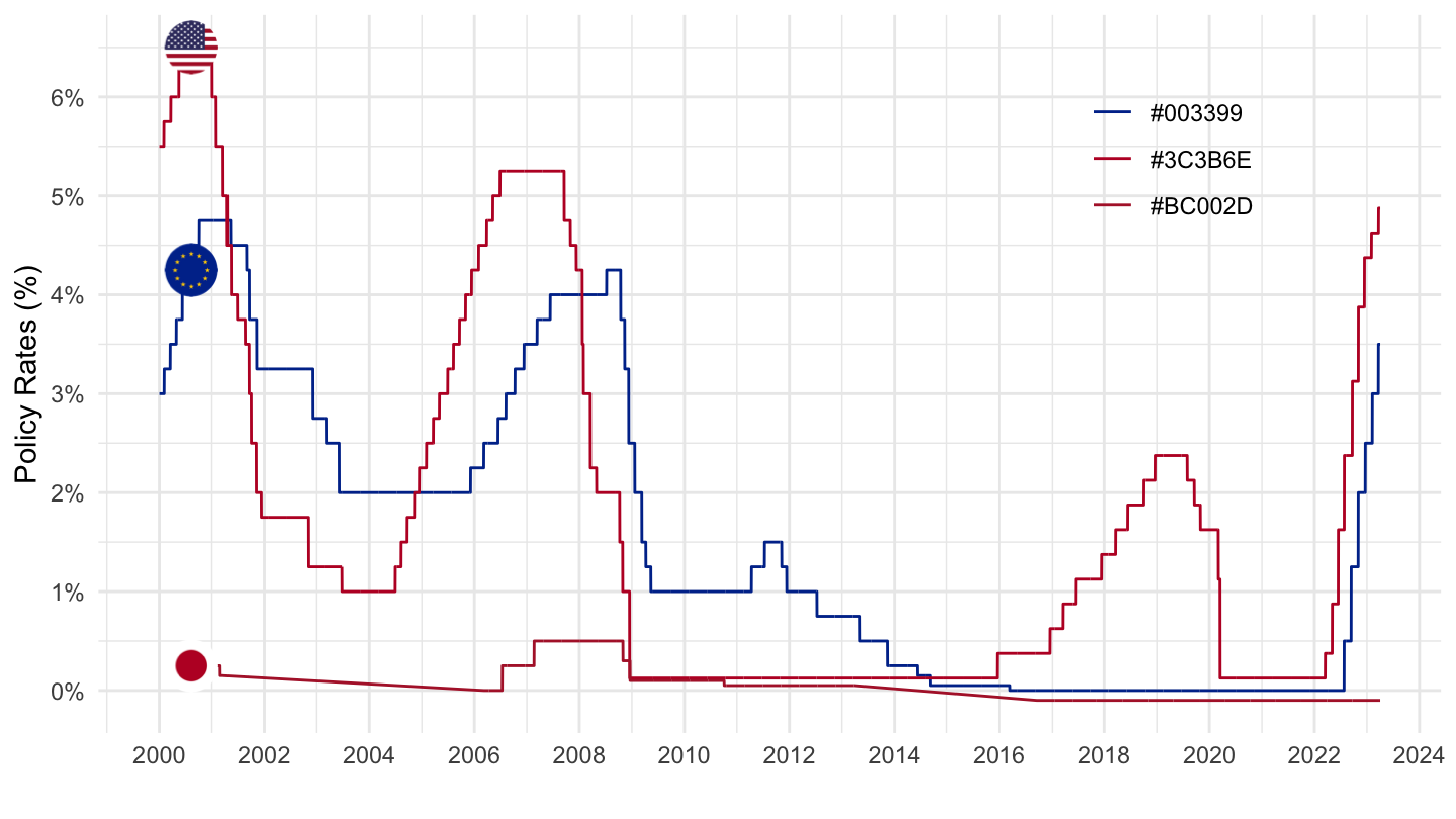
United States, Europe, Sweden
All
Code
CBPOL_D %>%
  left_join(REF_AREA, by = "REF_AREA") %>%
  filter(REF_AREA %in% c("US", "SE", "XM"),
         date >= as.Date("1998-01-01")) %>%
  mutate(`Reference area` = ifelse(REF_AREA == "XM", "Europe", `Reference area`)) %>%
  left_join(colors, by = c("Reference area" = "country")) %>%
  mutate(color = ifelse(REF_AREA == "US", color2, color)) %>%
  mutate(value = value/100, OBS_VALUE = value) %>%
  ggplot(.) + theme_minimal() + xlab("") + ylab("Policy Rates (%)") +
  geom_line(aes(x = date, y = value, color = color)) +
  scale_color_identity() + add_flags +
  scale_x_date(breaks = seq(1940, 2100, 2) %>% paste0("-01-01") %>% as.Date,
               labels = date_format("%Y")) +
  scale_y_continuous(breaks = 0.01*seq(-5, 30, 1),
                labels = percent_format(accuracy = 1)) +
  theme(legend.position = c(0.8, 0.80),
        legend.title = element_blank())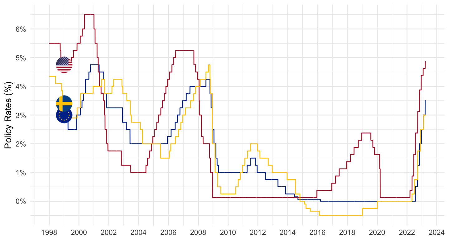
2000-
Code
CBPOL_D %>%

  left_join(REF_AREA, by = "REF_AREA") %>%
  filter(REF_AREA %in% c("US", "SE", "XM"),
         date >= as.Date("2000-01-01")) %>%
  mutate(`Reference area` = ifelse(REF_AREA == "XM", "Europe", `Reference area`)) %>%
  left_join(colors, by = c("Reference area" = "country")) %>%
  mutate(color = ifelse(REF_AREA == "US", color2, color)) %>%
  ggplot(.) + theme_minimal() + xlab("") + ylab("Policy Rates (%)") +
  geom_line(aes(x = date, y = value/100, color = color)) +
  scale_color_identity() + add_flags +
  scale_x_date(breaks = seq(1940, 2100, 2) %>% paste0("-01-01") %>% as.Date,
               labels = date_format("%Y")) +
  scale_y_continuous(breaks = 0.01*seq(-5, 30, 1),
                labels = percent_format(accuracy = 1)) +
  theme(legend.position = c(0.8, 0.80),
        legend.title = element_blank())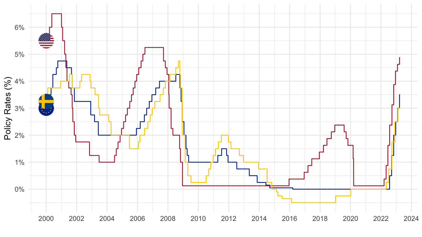
Switzerland, Denmark, United Kingdom
Code
CBPOL_D %>%

  left_join(REF_AREA, by = "REF_AREA") %>%
  filter(REF_AREA %in% c("CH", "DK", "GB")) %>%
  left_join(colors, by = c("Reference area" = "country")) %>%
  ggplot(.) + theme_minimal() + xlab("") + ylab("Policy Rates (%)") +
  geom_line(aes(x = date, y = value/100, color = color)) +
  scale_color_identity() + add_flags +
  scale_x_date(breaks = seq(1940, 2100, 5) %>% paste0("-01-01") %>% as.Date,
               labels = date_format("%Y")) +
  scale_y_continuous(breaks = 0.01*seq(-5, 30, 1),
                labels = percent_format(accuracy = 1)) +
  theme(legend.position = c(0.8, 0.80),
        legend.title = element_blank())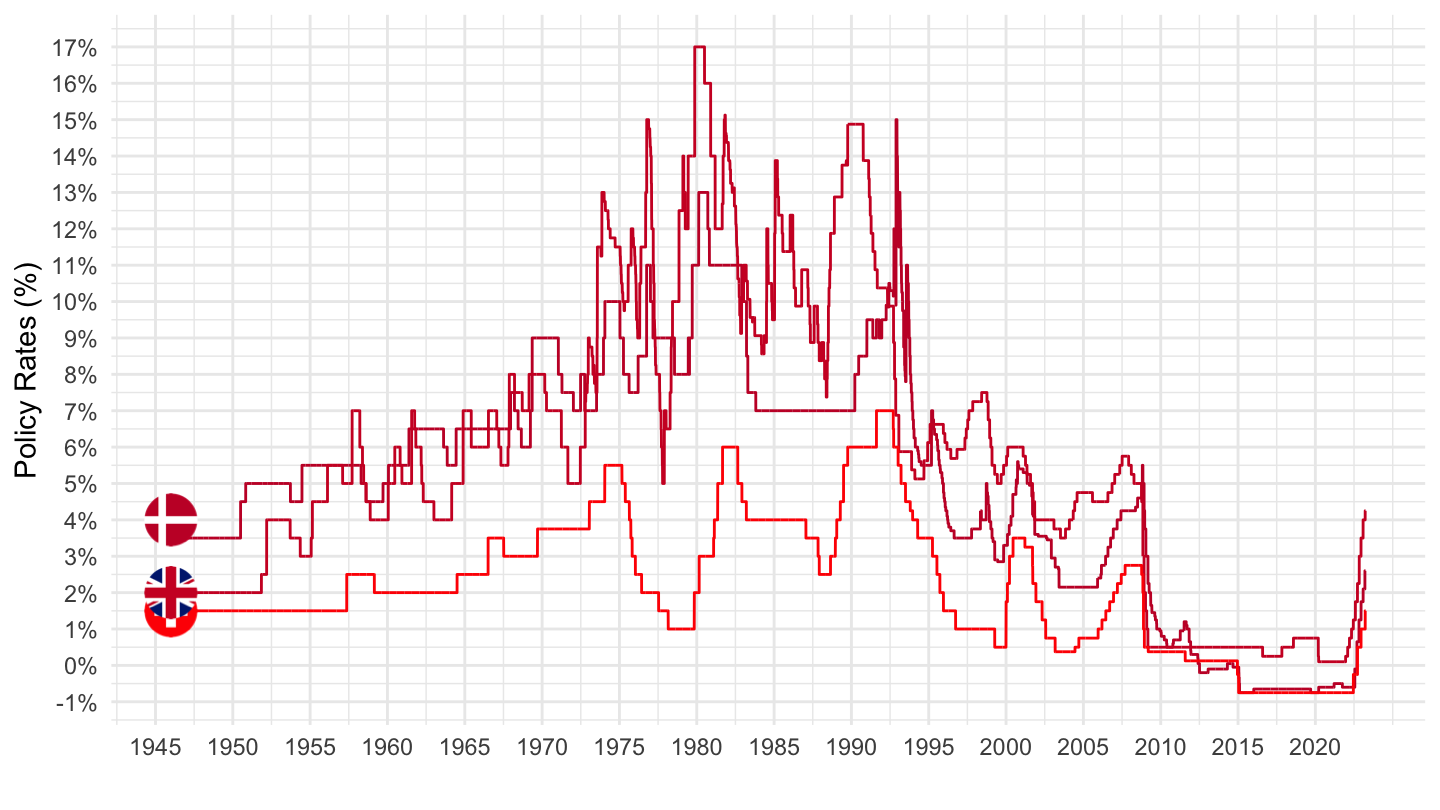
Sweden, India, United States
All
Code
CBPOL_D %>%

  left_join(REF_AREA, by = "REF_AREA") %>%
  filter(REF_AREA %in% c("SE", "IN", "US")) %>%
  left_join(colors, by = c("Reference area" = "country")) %>%
  ggplot(.) + theme_minimal() + xlab("") + ylab("Policy Rates (%)") +
  geom_line(aes(x = date, y = value/100, color = color)) +
  scale_color_identity() + add_flags +
  scale_x_date(breaks = seq(1940, 2100, 5) %>% paste0("-01-01") %>% as.Date,
               labels = date_format("%Y")) +
  scale_y_continuous(breaks = 0.01*seq(-5, 30, 1),
                labels = percent_format(accuracy = 1)) +
  theme(legend.position = c(0.8, 0.80),
        legend.title = element_blank())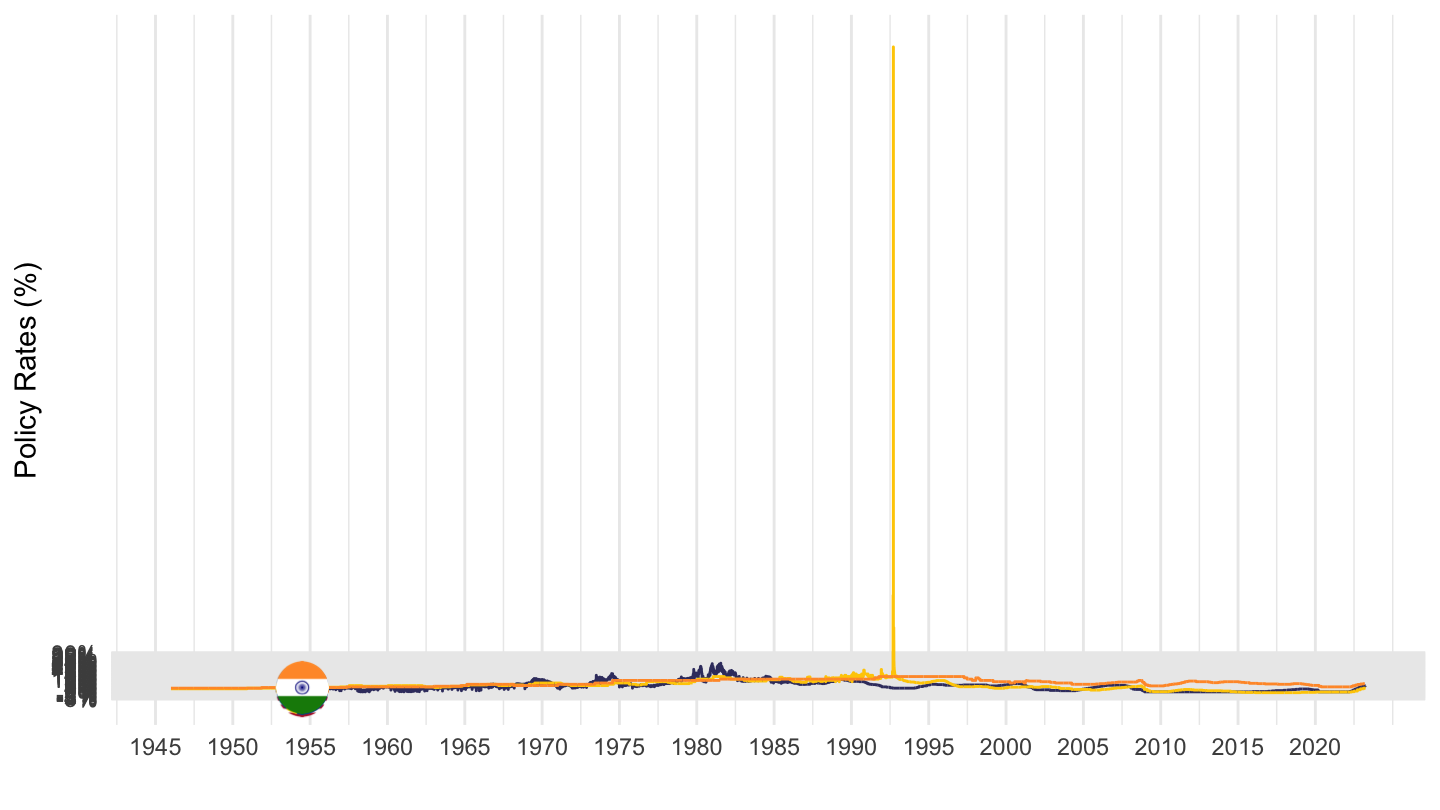
1993-
Code
CBPOL_D %>%

  left_join(REF_AREA, by = "REF_AREA") %>%
  filter(REF_AREA %in% c("SE", "IN", "US"),
         date >= as.Date("1993-01-01")) %>%
  left_join(colors, by = c("Reference area" = "country")) %>%
  ggplot(.) + theme_minimal() + xlab("") + ylab("Policy Rates (%)") +
  geom_line(aes(x = date, y = value/100, color = color)) +
  scale_color_identity() + add_flags +
  scale_x_date(breaks = seq(1940, 2100, 5) %>% paste0("-01-01") %>% as.Date,
               labels = date_format("%Y")) +
  scale_y_continuous(breaks = 0.01*seq(-5, 30, 1),
                labels = percent_format(accuracy = 1)) +
  theme(legend.position = c(0.8, 0.80),
        legend.title = element_blank())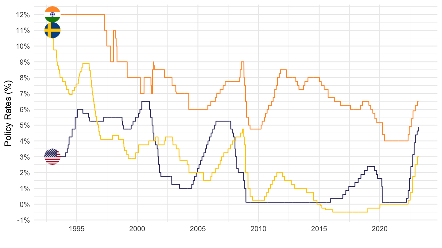
2000-
Code
CBPOL_D %>%

  left_join(REF_AREA, by = "REF_AREA") %>%
  filter(REF_AREA %in% c("SE", "IN", "US"),
         date >= as.Date("2000-01-01")) %>%
  left_join(colors, by = c("Reference area" = "country")) %>%
  ggplot(.) + theme_minimal() + xlab("") + ylab("Policy Rates (%)") +
  geom_line(aes(x = date, y = value/100, color = color)) +
  scale_color_identity() + add_flags +
  scale_x_date(breaks = seq(1940, 2100, 2) %>% paste0("-01-01") %>% as.Date,
               labels = date_format("%Y")) +
  scale_y_continuous(breaks = 0.01*seq(-5, 30, 1),
                labels = percent_format(accuracy = 1)) +
  theme(legend.position = c(0.8, 0.80),
        legend.title = element_blank())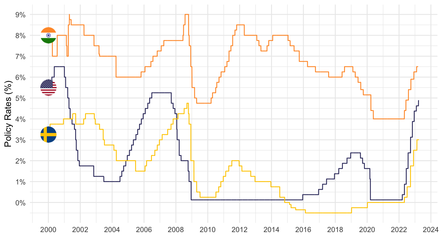
Japan, Canada, Australia
Code
CBPOL_D %>%

  left_join(REF_AREA, by = "REF_AREA") %>%
  filter(REF_AREA %in% c("JP", "CA", "AU")) %>%
  left_join(colors, by = c("Reference area" = "country")) %>%
  ggplot(.) + theme_minimal() + xlab("") + ylab("Policy Rates (%)") +
  geom_line(aes(x = date, y = value/100, color = color)) +
  scale_color_identity() + add_flags +
  scale_x_date(breaks = seq(1940, 2100, 5) %>% paste0("-01-01") %>% as.Date,
               labels = date_format("%Y")) +
  scale_y_continuous(breaks = 0.01*seq(-5, 100, 5),
                labels = percent_format(accuracy = 1)) +
  theme(legend.position = c(0.8, 0.80),
        legend.title = element_blank())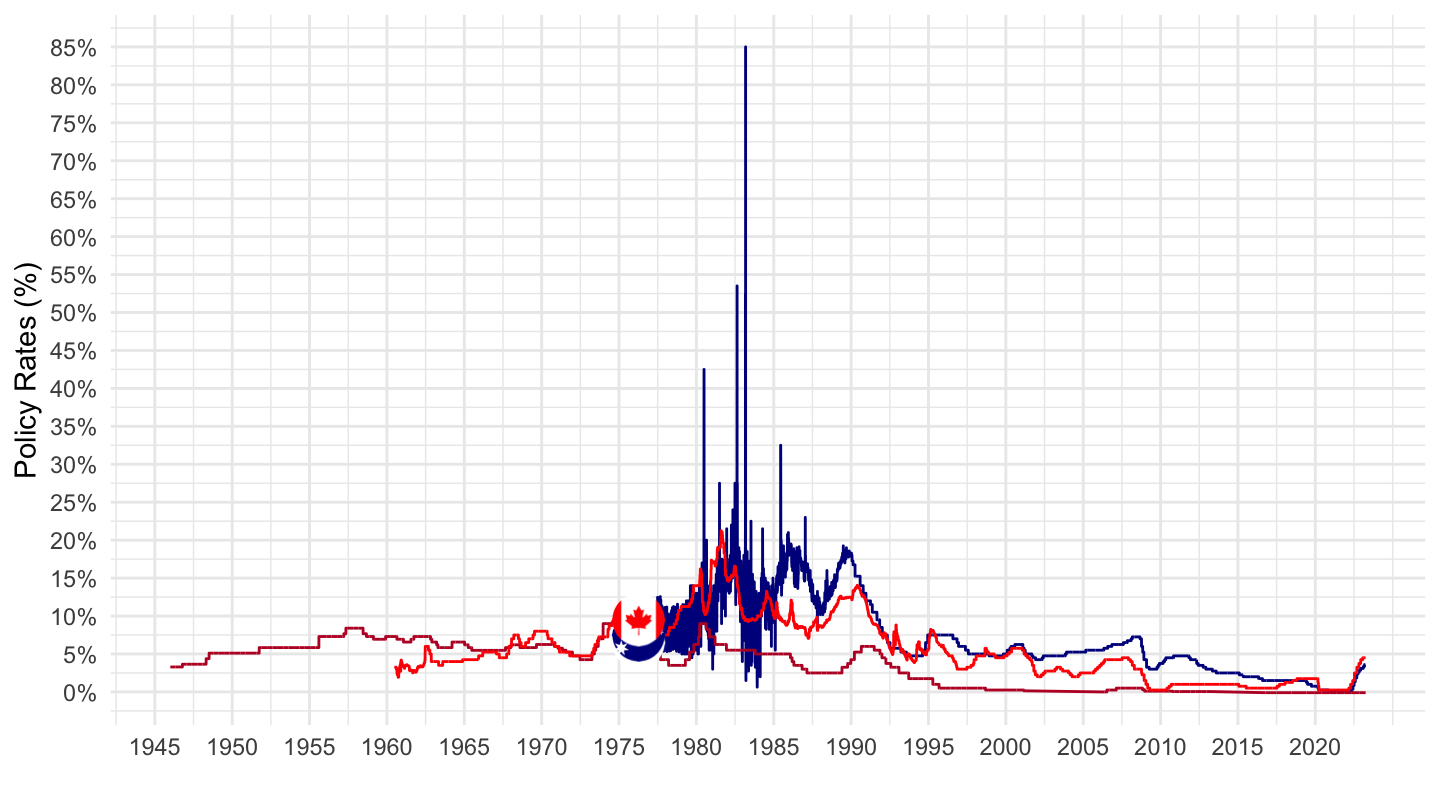
South Africa, New Zealand, Norway
Code
CBPOL_D %>%

  left_join(REF_AREA, by = "REF_AREA") %>%
  filter(REF_AREA %in% c("ZA", "NZ", "NO")) %>%
  left_join(colors, by = c("Reference area" = "country")) %>%
  ggplot(.) + theme_minimal() + xlab("") + ylab("Policy Rates (%)") +
  geom_line(aes(x = date, y = value/100, color = color)) +
  scale_color_identity() + add_flags +
  scale_x_date(breaks = seq(1940, 2100, 5) %>% paste0("-01-01") %>% as.Date,
               labels = date_format("%Y")) +
  scale_y_continuous(breaks = 0.01*seq(-5, 100, 5),
                labels = percent_format(accuracy = 1)) +
  theme(legend.position = c(0.8, 0.80),
        legend.title = element_blank())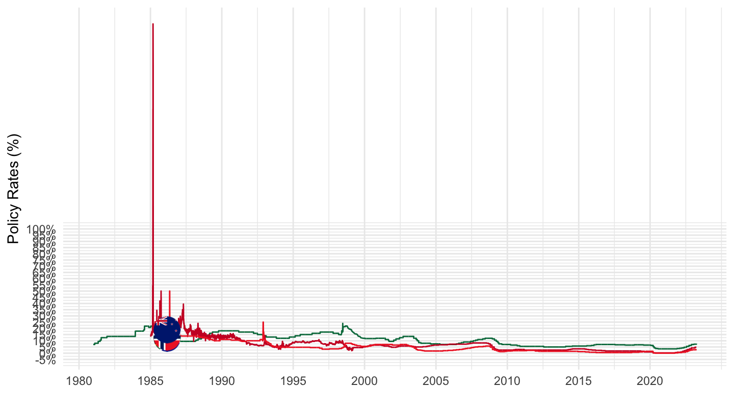
Brazil, Philippines, Hungary
Code
CBPOL_D %>%

  left_join(REF_AREA, by = "REF_AREA") %>%
  filter(REF_AREA %in% c("BR", "PH", "HU")) %>%
  left_join(colors, by = c("Reference area" = "country")) %>%
  ggplot(.) + theme_minimal() + xlab("") + ylab("Policy Rates (%)") +
  geom_line(aes(x = date, y = value/100, color = color)) +
  scale_color_identity() + add_flags +
  scale_x_date(breaks = seq(1940, 2100, 5) %>% paste0("-01-01") %>% as.Date,
               labels = date_format("%Y")) +
  scale_y_continuous(breaks = 0.01*seq(-5, 100, 5),
                labels = percent_format(accuracy = 1),
                limits = c(-0.05, 0.40)) +
  theme(legend.position = c(0.8, 0.80),
        legend.title = element_blank())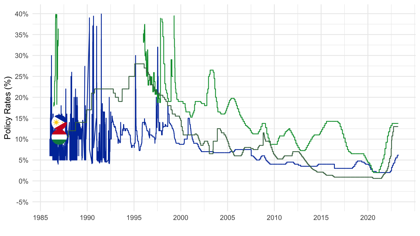
Russia, Poland, Argentina
All
Code
CBPOL_D %>%

  left_join(REF_AREA, by = "REF_AREA") %>%
  filter(REF_AREA %in% c("RU", "PL", "AR")) %>%
  left_join(colors, by = c("Reference area" = "country")) %>%
  ggplot(.) + theme_minimal() + xlab("") + ylab("Policy Rates (%)") +
  geom_line(aes(x = date, y = value/100, color = color)) +
  scale_color_identity() + add_flags +
  scale_x_date(breaks = seq(1940, 2100, 5) %>% paste0("-01-01") %>% as.Date,
               labels = date_format("%Y")) +
  scale_y_continuous(breaks = 0.01*seq(0, 10000, 50),
                labels = percent_format(accuracy = 1)) +
  theme(legend.position = c(0.8, 0.80),
        legend.title = element_blank())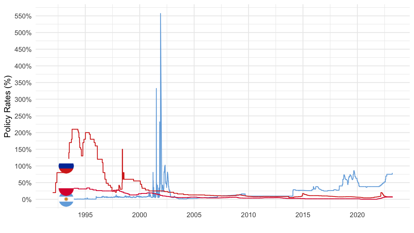
1990-
Code
CBPOL_D %>%

  left_join(REF_AREA, by = "REF_AREA") %>%
  filter(REF_AREA %in% c("RU", "PL", "AR"),
         date >= as.Date("2006-01-01")) %>%
  left_join(colors, by = c("Reference area" = "country")) %>%
  ggplot(.) + theme_minimal() + xlab("") + ylab("Policy Rates (%)") +
  geom_line(aes(x = date, y = value/100, color = color)) +
  scale_color_identity() + add_flags +
  scale_x_date(breaks = seq(1940, 2100, 2) %>% paste0("-01-01") %>% as.Date,
               labels = date_format("%Y")) +
  scale_y_continuous(breaks = 0.01*seq(0, 10000, 10),
                labels = percent_format(accuracy = 1)) +
  theme(legend.position = c(0.8, 0.80),
        legend.title = element_blank())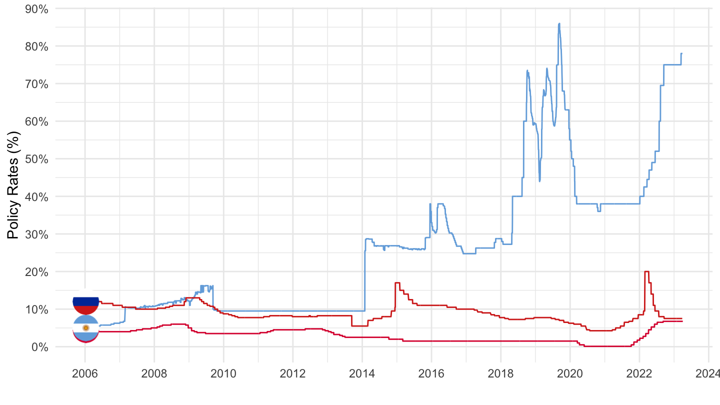
Israel, Colombia, Croatia
Code
CBPOL_D %>%

  left_join(REF_AREA, by = "REF_AREA") %>%
  filter(REF_AREA %in% c("IL", "CO", "HR")) %>%
  left_join(colors, by = c("Reference area" = "country")) %>%
  ggplot(.) + theme_minimal() + xlab("") + ylab("Policy Rates (%)") +
  geom_line(aes(x = date, y = value/100, color = color)) +
  scale_color_identity() + add_flags +
  scale_x_date(breaks = seq(1940, 2100, 5) %>% paste0("-01-01") %>% as.Date,
               labels = date_format("%Y")) +
  scale_y_continuous(breaks = 0.01*seq(0, 10000, 50),
                labels = percent_format(accuracy = 1)) +
  theme(legend.position = c(0.8, 0.80),
        legend.title = element_blank())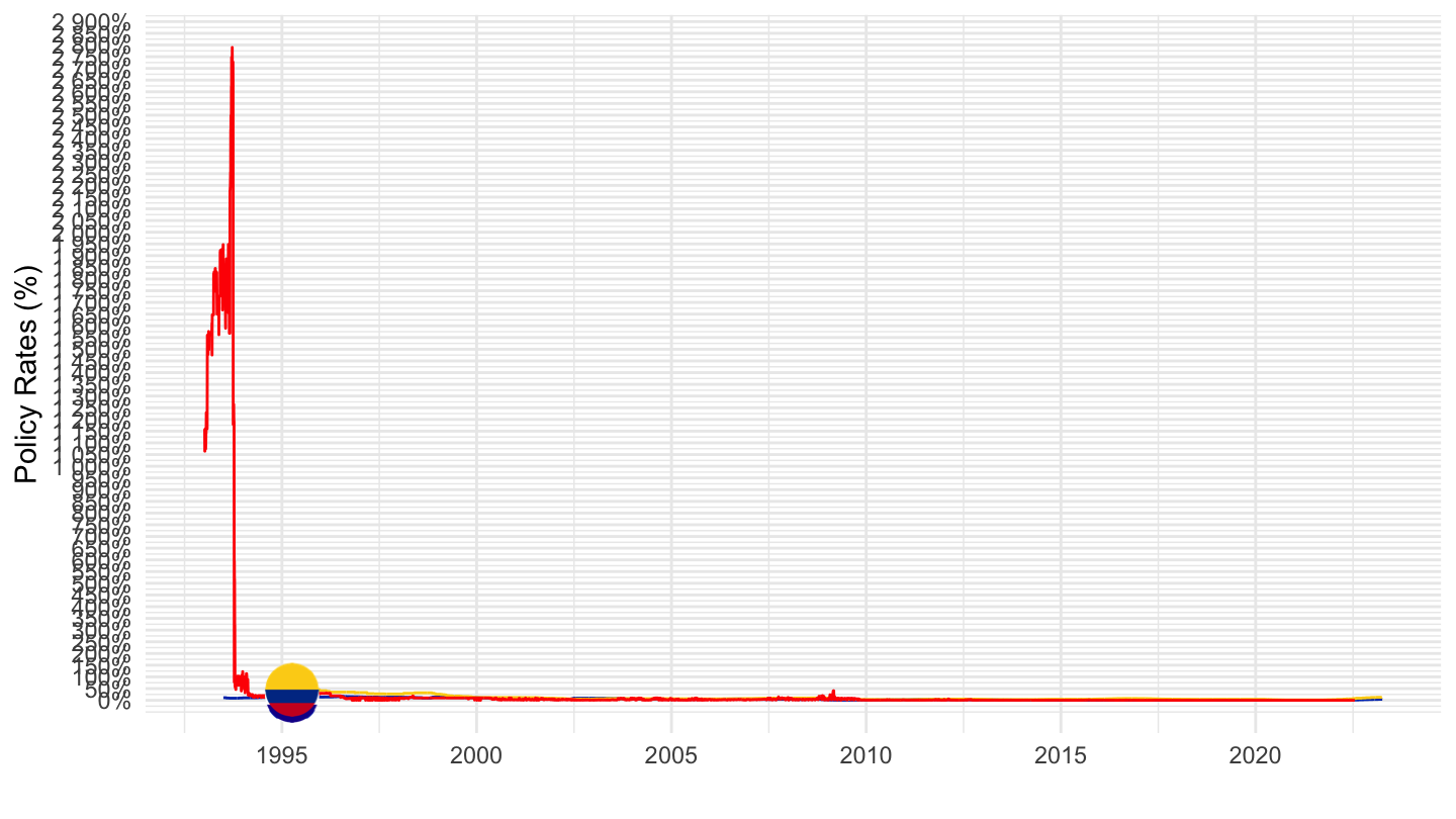
Malaysia, Czech Republic, China
Code
CBPOL_D %>%

  left_join(REF_AREA, by = "REF_AREA") %>%
  filter(REF_AREA %in% c("MY", "CZ", "CN")) %>%
  left_join(colors, by = c("Reference area" = "country")) %>%
  ggplot(.) + theme_minimal() + xlab("") + ylab("Policy Rates (%)") +
  geom_line(aes(x = date, y = value/100, color = color)) +
  scale_color_identity() + add_flags +
  scale_x_date(breaks = seq(1940, 2100, 5) %>% paste0("-01-01") %>% as.Date,
               labels = date_format("%Y")) +
  scale_y_continuous(breaks = 0.01*seq(0, 10000, 1),
                labels = percent_format(accuracy = 1)) +
  theme(legend.position = c(0.8, 0.80),
        legend.title = element_blank())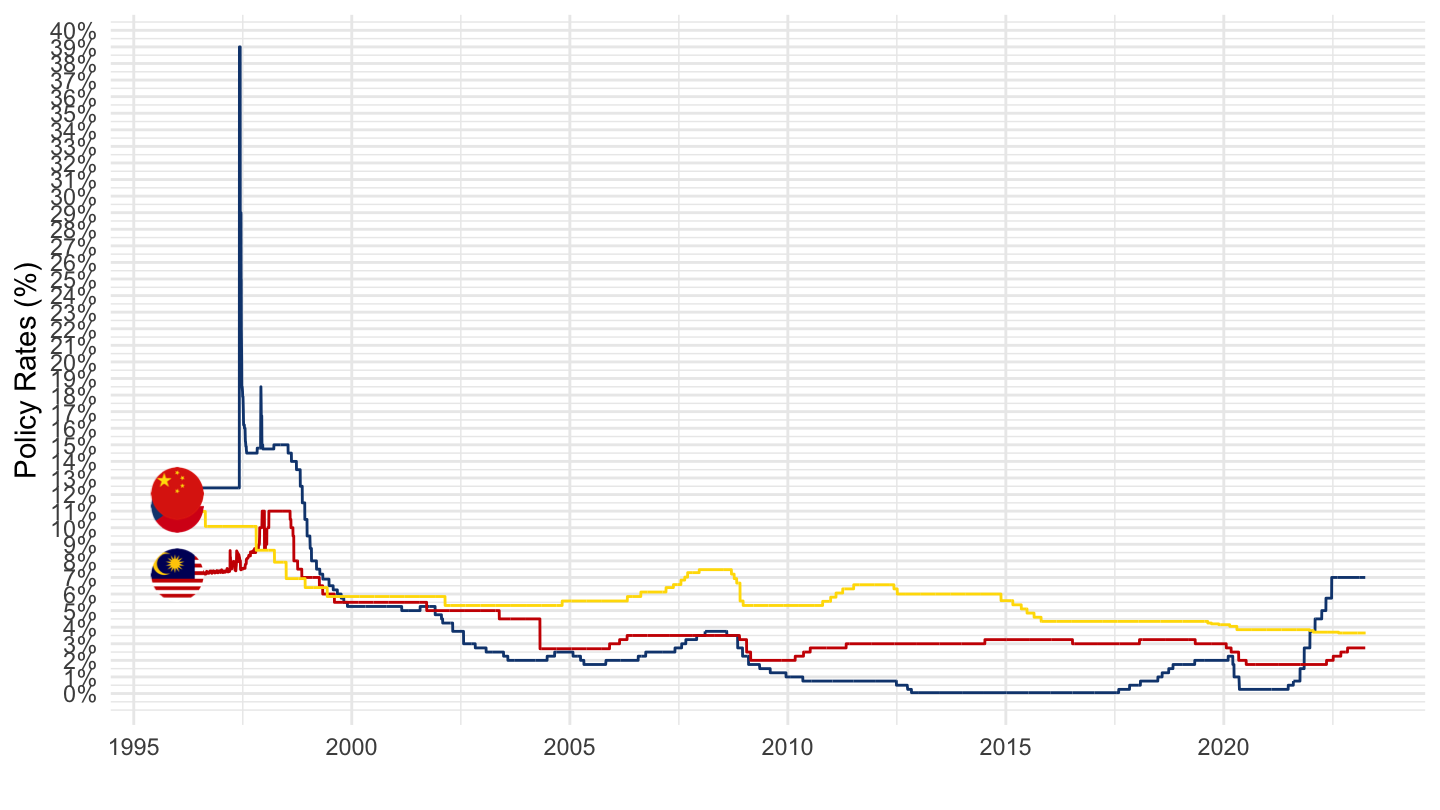
Serbia, Chile, Iceland
Code
CBPOL_D %>%

  left_join(REF_AREA, by = "REF_AREA") %>%
  filter(REF_AREA %in% c("RS", "CL", "IS")) %>%
  left_join(colors, by = c("Reference area" = "country")) %>%
  ggplot(.) + theme_minimal() + xlab("") + ylab("Policy Rates (%)") +
  geom_line(aes(x = date, y = value/100, color = color)) +
  scale_color_identity() + add_flags +
  scale_x_date(breaks = seq(1940, 2100, 5) %>% paste0("-01-01") %>% as.Date,
               labels = date_format("%Y")) +
  scale_y_continuous(breaks = 0.01*seq(0, 10000, 5),
                labels = percent_format(accuracy = 1)) +
  theme(legend.position = c(0.8, 0.80),
        legend.title = element_blank())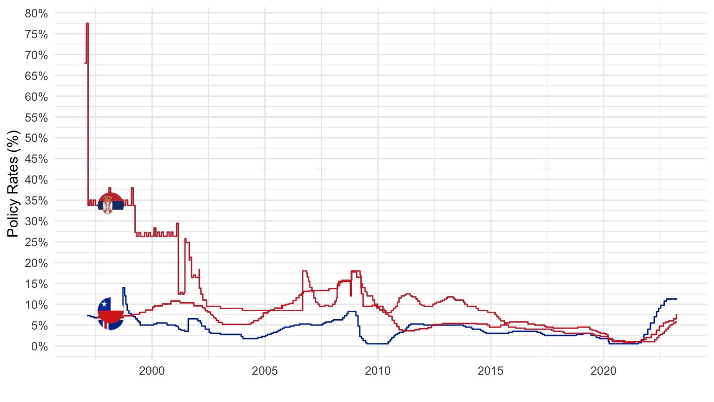
Hong Kong, Mexico, Euro area
Code
CBPOL_D %>%

  left_join(REF_AREA, by = "REF_AREA") %>%
  filter(REF_AREA %in% c("HK", "MX", "XM")) %>%
  mutate(`Reference area` = ifelse(REF_AREA == "XM", "Europe", `Reference area`)) %>%
  mutate(`Reference area` = ifelse(REF_AREA == "HK", "Hong Kong", `Reference area`)) %>%
  left_join(colors, by = c("Reference area" = "country")) %>%
  ggplot(.) + theme_minimal() + xlab("") + ylab("Policy Rates (%)") +
  geom_line(aes(x = date, y = value/100, color = color)) +
  scale_color_identity() + add_flags +
  scale_x_date(breaks = seq(1940, 2100, 5) %>% paste0("-01-01") %>% as.Date,
               labels = date_format("%Y")) +
  scale_y_continuous(breaks = 0.01*seq(0, 10000, 5),
                labels = percent_format(accuracy = 1)) +
  theme(legend.position = c(0.8, 0.80),
        legend.title = element_blank())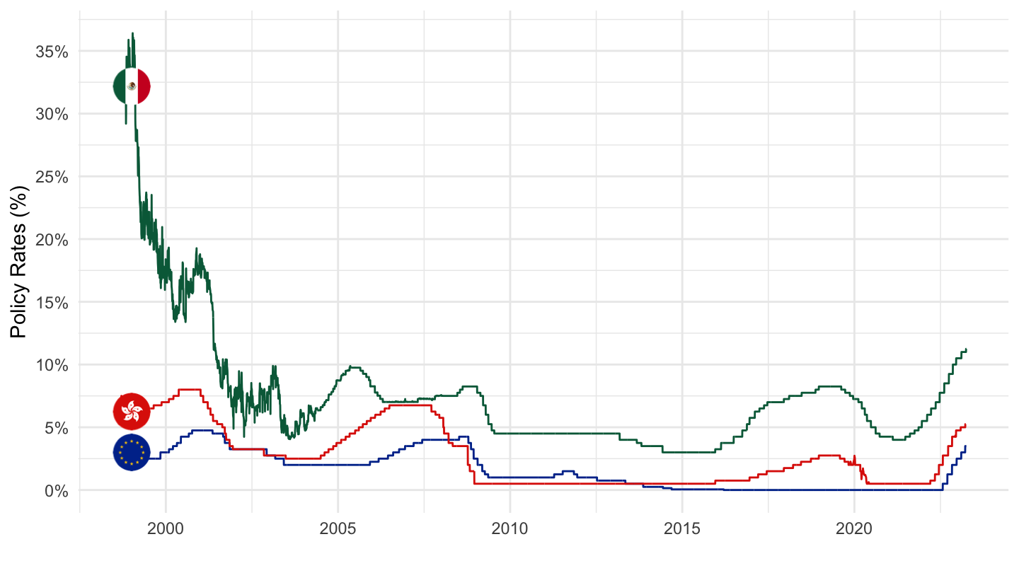
South Korea, North Macedonia, Saudi Arabia
Code
CBPOL_D %>%

  left_join(REF_AREA, by = "REF_AREA") %>%
  filter(REF_AREA %in% c("KR", "MK", "SA")) %>%
  left_join(colors, by = c("Reference area" = "country")) %>%
  ggplot(.) + theme_minimal() + xlab("") + ylab("Policy Rates (%)") +
  geom_line(aes(x = date, y = value/100, color = color)) +
  scale_color_identity() + add_flags +
  scale_x_date(breaks = seq(1940, 2100, 5) %>% paste0("-01-01") %>% as.Date,
               labels = date_format("%Y")) +
  scale_y_continuous(breaks = 0.01*seq(0, 10000, 5),
                labels = percent_format(accuracy = 1)) +
  theme(legend.position = c(0.8, 0.80),
        legend.title = element_blank())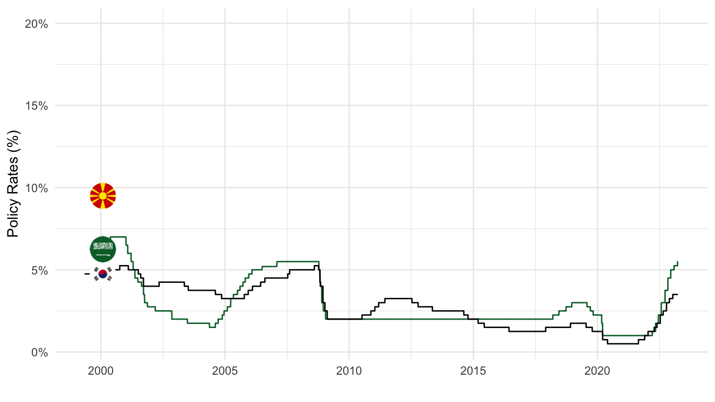
Thailand, Turkey, Romania
Code
CBPOL_D %>%

  left_join(REF_AREA, by = "REF_AREA") %>%
  filter(REF_AREA %in% c("TH", "TR", "RO")) %>%
  left_join(colors, by = c("Reference area" = "country")) %>%
  ggplot(.) + theme_minimal() + xlab("") + ylab("Policy Rates (%)") +
  geom_line(aes(x = date, y = value/100, color = color)) +
  scale_color_identity() +
  scale_x_date(breaks = seq(1940, 2100, 5) %>% paste0("-01-01") %>% as.Date,
               labels = date_format("%Y")) +
  scale_y_continuous(breaks = 0.01*seq(0, 10000, 5),
                labels = percent_format(accuracy = 1)) +
  theme(legend.position = c(0.8, 0.80),
        legend.title = element_blank())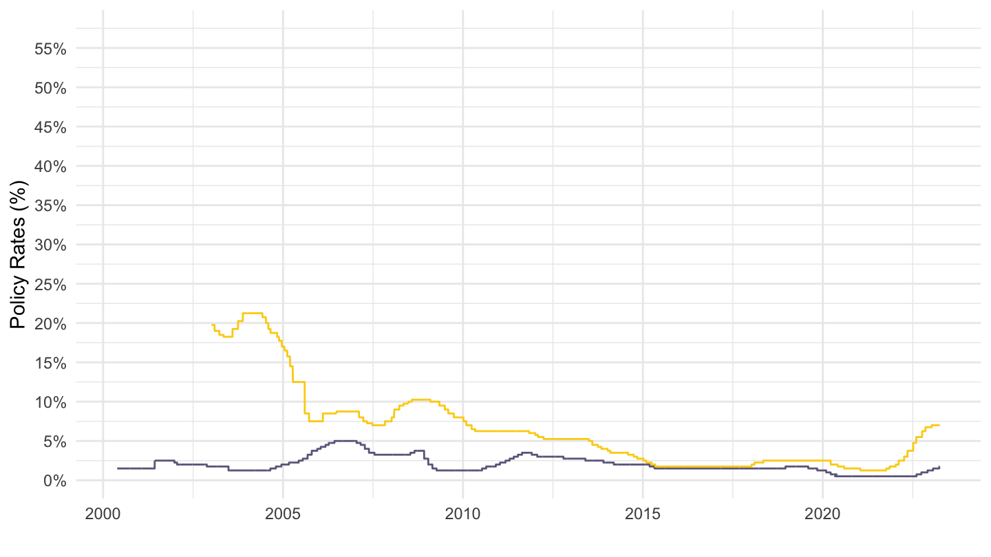
South Korea, Brazil, Turkey
1995-
Code
CBPOL_D %>%

  left_join(REF_AREA, by = "REF_AREA") %>%
  filter(REF_AREA %in% c("KR", "BR", "TR"),
         date >= as.Date("1995-01-01")) %>%
  left_join(colors, by = c("Reference area" = "country")) %>%
  ggplot(.) + theme_minimal() + xlab("") + ylab("Policy Rates (%)") +
  geom_line(aes(x = date, y = value/100, color = color)) +
  scale_color_identity() +
  scale_x_date(breaks = seq(1940, 2100, 1) %>% paste0("-01-01") %>% as.Date,
               labels = date_format("%Y")) +
  scale_y_continuous(breaks = 0.01*seq(0, 10000, 5),
                labels = percent_format(accuracy = 1)) +
  theme(legend.position = c(0.8, 0.80),
        legend.title = element_blank())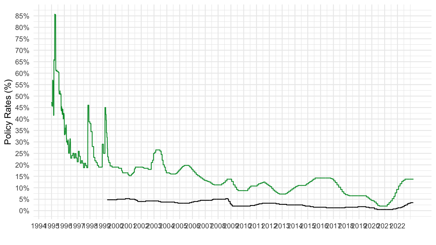
2015-
Code
CBPOL_D %>%

  left_join(REF_AREA, by = "REF_AREA") %>%
  filter(REF_AREA %in% c("KR", "BR", "TR"),
         date >= as.Date("2015-01-01")) %>%
  left_join(colors, by = c("Reference area" = "country")) %>%
  ggplot(.) + theme_minimal() + xlab("") + ylab("Policy Rates (%)") +
  geom_line(aes(x = date, y = value/100, color = color)) +
  scale_color_identity() +
  scale_x_date(breaks = seq(1940, 2100, 1) %>% paste0("-01-01") %>% as.Date,
               labels = date_format("%Y")) +
  scale_y_continuous(breaks = 0.01*seq(0, 10000, 5),
                labels = percent_format(accuracy = 1)) +
  theme(legend.position = c(0.8, 0.80),
        legend.title = element_blank())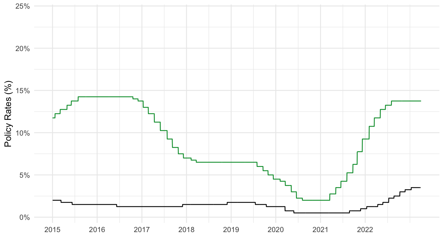
More…
Data on monetary-policy
| source | dataset | Title | .html | .rData |
|---|---|---|---|---|
| bdf | FM | Marché financier, taux | 2026-07-24 | 2026-07-24 |
| bdf | MIR | Taux d'intérêt - Zone euro | 2026-07-24 | 2026-07-24 |
| bdf | MIR1 | Taux d'intérêt - France | 2026-07-24 | 2026-07-24 |
| bis | CBPOL | Policy Rates, Daily | 2026-07-18 | 2026-07-24 |
| ecb | BSI | Balance Sheet Items | 2026-07-24 | 2026-07-23 |
| ecb | BSI_PUB | Balance Sheet Items - Published series | 2026-07-24 | 2026-07-24 |
| ecb | FM | Financial market data | 2026-07-24 | 2026-07-24 |
| ecb | ILM | Internal Liquidity Management | 2026-07-24 | 2026-07-24 |
| ecb | ILM_PUB | Internal Liquidity Management - Published series | 2026-07-24 | 2026-07-24 |
| ecb | MIR | MFI Interest Rate Statistics | 2026-07-24 | 2026-07-24 |
| ecb | RAI | Risk Assessment Indicators | 2026-07-24 | 2026-07-24 |
| ecb | SUP | Supervisory Banking Statistics | 2026-07-24 | 2026-07-24 |
| ecb | YC | Financial market data - yield curve | 2026-07-24 | 2026-07-23 |
| ecb | YC_PUB | Financial market data - yield curve - Published series | 2026-07-24 | 2026-07-24 |
| ecb | liq_daily | Daily Liquidity | 2026-07-24 | 2026-07-24 |
| eurostat | ei_mfir_m | Interest rates - monthly data | 2026-07-23 | 2026-07-23 |
| eurostat | irt_st_m | Money market interest rates - monthly data | 2026-07-24 | 2026-07-23 |
| fred | r | Interest Rates | 2026-07-24 | 2026-07-24 |
| oecd | MEI | Main Economic Indicators | 2026-07-24 | 2025-07-24 |
| oecd | MEI_FIN | Monthly Monetary and Financial Statistics (MEI) | 2024-09-15 | 2025-07-24 |
Data on interest rates
| source | dataset | Title | .html | .rData |
|---|---|---|---|---|
| bis | CBPOL_D | Policy Rates, Daily | 2026-07-18 | 2025-08-20 |
| bdf | FM | Marché financier, taux | 2026-07-24 | 2026-07-24 |
| bdf | MIR | Taux d'intérêt - Zone euro | 2026-07-24 | 2026-07-24 |
| bdf | MIR1 | Taux d'intérêt - France | 2026-07-24 | 2026-07-24 |
| bis | CBPOL_M | Policy Rates, Monthly | 2026-07-24 | 2024-04-19 |
| ecb | FM | Financial market data | 2026-07-24 | 2026-07-24 |
| ecb | MIR | MFI Interest Rate Statistics | 2026-07-24 | 2026-07-24 |
| eurostat | ei_mfir_m | Interest rates - monthly data | 2026-07-23 | 2026-07-23 |
| eurostat | irt_lt_mcby_d | EMU convergence criterion series - daily data | 2026-07-24 | 2025-07-24 |
| eurostat | irt_st_m | Money market interest rates - monthly data | 2026-07-24 | 2026-07-23 |
| fred | r | Interest Rates | 2026-07-24 | 2026-07-24 |
| oecd | MEI | Main Economic Indicators | 2026-07-24 | 2025-07-24 |
| oecd | MEI_FIN | Monthly Monetary and Financial Statistics (MEI) | 2024-09-15 | 2025-07-24 |
| wdi | FR.INR.DPST | Deposit interest rate (%) | 2026-07-24 | 2026-07-24 |
| wdi | FR.INR.LEND | Lending interest rate (%) | 2026-07-24 | 2026-07-24 |
| wdi | FR.INR.RINR | Real interest rate (%) | 2026-07-24 | 2026-07-24 |