| source | dataset | Title | .html | .rData |
|---|---|---|---|---|
| wdi | SL.TLF.PART.ZS | Part-Time Employment Rate (%) | 2026-07-04 | 2026-06-20 |
Part-Time Employment Rate (%)
Data - WDI
Info
Data on macro
| source | dataset | Title | .html | .rData |
|---|---|---|---|---|
| eurostat | nama_10_a10 | Gross value added and income by A*10 industry breakdowns | 2026-06-20 | 2026-04-26 |
| eurostat | nama_10_a10_e | Employment by A*10 industry breakdowns | 2026-06-20 | 2026-04-26 |
| eurostat | nama_10_gdp | GDP and main components (output, expenditure and income) | 2026-06-20 | 2026-04-26 |
| eurostat | nama_10_lp_ulc | Labour productivity and unit labour costs | 2026-06-20 | 2026-04-26 |
| eurostat | namq_10_a10 | Gross value added and income A*10 industry breakdowns | 2026-06-03 | 2026-06-03 |
| eurostat | namq_10_a10_e | Employment A*10 industry breakdowns | 2025-05-24 | 2026-04-26 |
| eurostat | namq_10_gdp | GDP and main components (output, expenditure and income) | 2025-10-27 | 2026-04-26 |
| eurostat | namq_10_lp_ulc | Labour productivity and unit labour costs | 2026-06-21 | 2026-04-26 |
| eurostat | namq_10_pc | Main GDP aggregates per capita | 2026-03-24 | 2026-04-26 |
| eurostat | nasa_10_nf_tr | Non-financial transactions | 2026-06-21 | 2026-04-26 |
| eurostat | nasq_10_nf_tr | Non-financial transactions | 2026-06-21 | 2026-04-26 |
| fred | gdp | Gross Domestic Product | 2026-07-04 | 2026-07-04 |
| oecd | QNA | Quarterly National Accounts | 2026-06-21 | 2026-06-19 |
| oecd | SNA_TABLE1 | Gross domestic product (GDP) | 2026-06-21 | 2025-05-24 |
| oecd | SNA_TABLE14A | Non-financial accounts by sectors | 2026-06-21 | 2024-06-30 |
| oecd | SNA_TABLE2 | Disposable income and net lending - net borrowing | 2024-07-01 | 2024-04-11 |
| oecd | SNA_TABLE6A | Value added and its components by activity, ISIC rev4 | 2024-07-01 | 2024-06-30 |
| wdi | NE.RSB.GNFS.ZS | External balance on goods and services (% of GDP) | 2026-07-04 | 2026-06-20 |
| wdi | NY.GDP.MKTP.CD | NA | NA | NA |
| wdi | NY.GDP.MKTP.PP.CD | GDP, PPP (current international D) | 2026-07-04 | 2026-06-20 |
| wdi | NY.GDP.PCAP.CD | GDP per capita (current USD) | 2026-07-04 | 2026-06-20 |
| wdi | NY.GDP.PCAP.KD | GDP per capita (constant 2015 USD) | 2026-07-04 | 2026-06-20 |
| wdi | NY.GDP.PCAP.PP.CD | GDP per capita, PPP (current international D) | 2026-02-23 | 2026-06-20 |
| wdi | NY.GDP.PCAP.PP.KD | GDP per capita, PPP (constant 2011 international D) | 2026-07-04 | 2026-06-20 |
LAST_COMPILE
| LAST_COMPILE |
|---|
| 2026-07-04 |
Last
Code
SL.TLF.PART.ZS %>%
  group_by(year) %>%
  summarise(Nobs = n()) %>%
  arrange(desc(year)) %>%
  head(1) %>%
print_table_conditional()| year | Nobs |
|---|---|
| 2024 | 102 |
Nobs - Javascript
Code
SL.TLF.PART.ZS %>%
  left_join(iso2c, by = "iso2c") %>%
  group_by(iso2c, Iso2c) %>%

  mutate(value = round(value/(10^9))) %>%
  summarise(Nobs = n(),
            `Year 1` = first(year),
            `GDP 1 (Bn)` = first(value) %>% paste0("$ ", .),
            `Year 2` = last(year),
            `GDP 2 (Bn)` = last(value) %>% paste0("$ ", .)) %>%
  arrange(-Nobs) %>%
  mutate(Flag = gsub(" ", "-", str_to_lower(Iso2c)),
         Flag = paste0('<img src="../../bib/flags/vsmall/', Flag, '.png" alt="Flag">')) %>%
  select(Flag, everything()) %>%
  {if (is_html_output()) datatable(., filter = 'top', rownames = F, escape = F) else .}
Germany, France, Italy, Spain
Code
SL.TLF.PART.ZS %>%
  right_join(iso2c, by = "iso2c") %>%
  filter(iso2c %in% c("DE", "FR", "IT", "ES", "GB")) %>%
  year_to_date %>%
  mutate(value = value/100) %>%
  left_join(colors, by = c("Iso2c" = "country")) %>%
  ggplot(.) + theme_minimal() + scale_color_identity() + xlab("") + ylab("% of World GDP") +
  geom_line(aes(x = date, y = value, color = color)) + add_5flags +
  scale_x_date(breaks = seq(1950, 2100, 5) %>% paste0("-01-01") %>% as.Date,
               labels = date_format("%Y")) +
  scale_y_continuous(breaks = 0.01*seq(0, 100, 2),
                     labels = scales::percent_format(accuracy = 1))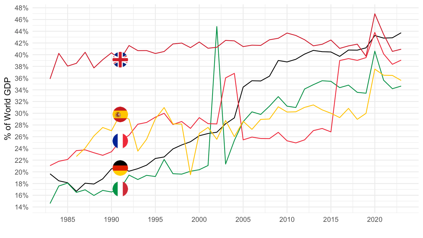
US, Euro Area
All
Code
SL.TLF.PART.ZS %>%
  right_join(iso2c, by = "iso2c") %>%
  filter(iso2c %in% c("US", "XC")) %>%
  year_to_date %>%
  mutate(value = value/100) %>%
  mutate(Iso2c = ifelse(iso2c == "XC", "Europe", Iso2c)) %>%
  left_join(colors, by = c("Iso2c" = "country")) %>%
  mutate(color = ifelse(iso2c == "US", color2, color)) %>%
  ggplot(.) + theme_minimal() + scale_color_identity() + xlab("") +
  ylab("Taux d'emploi à temps partiel (% de l'emploi total)") +
  geom_line(aes(x = date, y = value, color = color)) + add_2flags +
  scale_x_date(breaks = seq(1950, 2100, 5) %>% paste0("-01-01") %>% as.Date,
               labels = date_format("%Y")) +
  scale_y_continuous(breaks = 0.01*seq(0, 100, 2),
                     labels = scales::percent_format(accuracy = 1))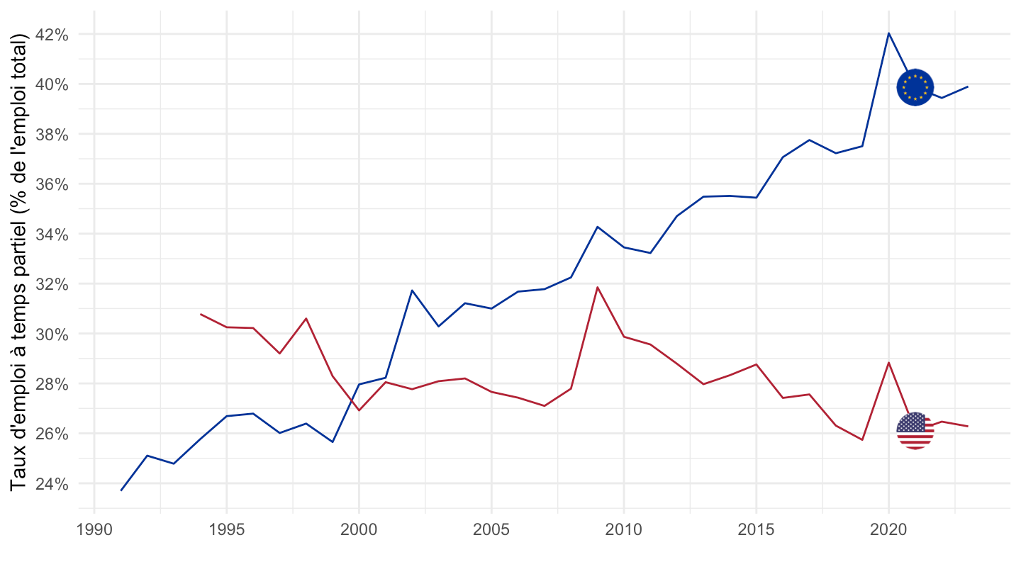
1999-
Code
SL.TLF.PART.ZS %>%
  right_join(iso2c, by = "iso2c") %>%
  filter(iso2c %in% c("US", "XC")) %>%
  year_to_date %>%
  mutate(value = value/100) %>%
  filter(date >= as.Date("1999-01-01")) %>%
  mutate(Iso2c = ifelse(iso2c == "XC", "Europe", Iso2c)) %>%
  left_join(colors, by = c("Iso2c" = "country")) %>%
  mutate(color = ifelse(iso2c == "US", color2, color)) %>%
  ggplot(.) + theme_minimal() + scale_color_identity() + xlab("") +
  ylab("Part de l'emploi à temps partiel (% de l'emploi total)") +
  geom_line(aes(x = date, y = value, color = color)) + add_2flags +
  scale_x_date(breaks = c(seq(1999, 2100, 5), seq(1997, 2100, 5)) %>% paste0("-01-01") %>% as.Date,
               labels = date_format("%Y")) +
  scale_y_continuous(breaks = 0.01*seq(0, 100, 2),
                     labels = scales::percent_format(accuracy = 1))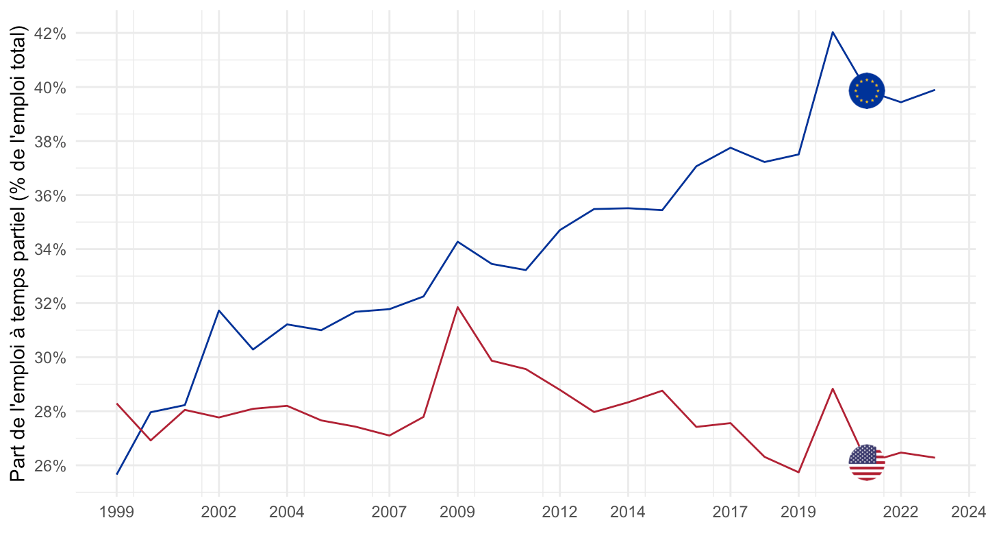
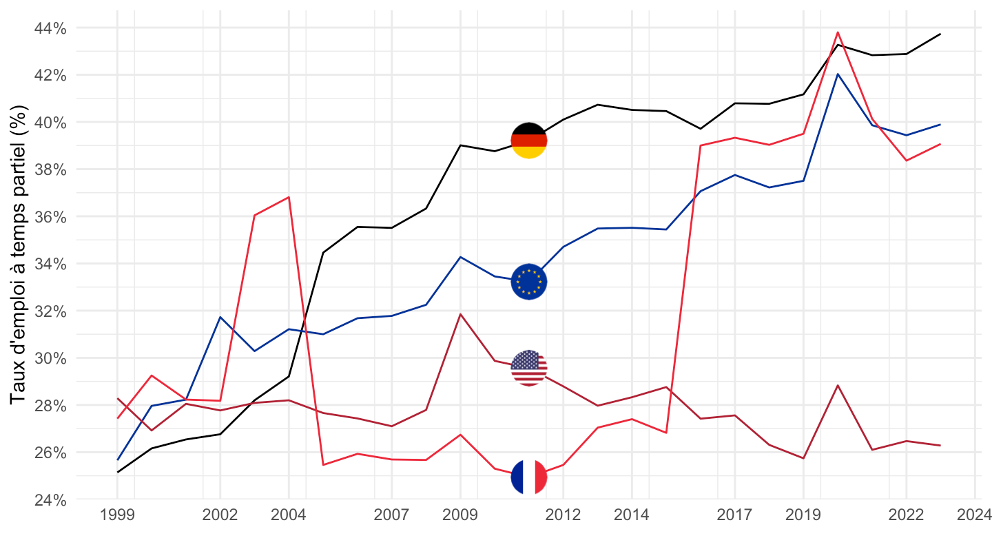
France, Germany, Euro area, US
All
Code
SL.TLF.PART.ZS %>%
  right_join(iso2c, by = "iso2c") %>%
  filter(iso2c %in% c("US", "XC", "FR", "DE")) %>%
  year_to_date %>%
  mutate(value = value/100) %>%
  #filter(date >= as.Date("1999-01-01")) %>%
  mutate(Iso2c = ifelse(iso2c == "XC", "Europe", Iso2c)) %>%
  left_join(colors, by = c("Iso2c" = "country")) %>%
  mutate(color = ifelse(iso2c == "US", color2, color)) %>%
  ggplot(.) + theme_minimal() + scale_color_identity() + xlab("") +
  ylab("Taux d'emploi à temps partiel (%)") +
  geom_line(aes(x = date, y = value, color = color)) + add_4flags +
  scale_x_date(breaks = c(seq(1949, 2100, 5), seq(1947, 2100, 5)) %>% paste0("-01-01") %>% as.Date,
               labels = date_format("%Y")) +
  scale_y_continuous(breaks = 0.01*seq(0, 100, 2),
                     labels = scales::percent_format(accuracy = 1))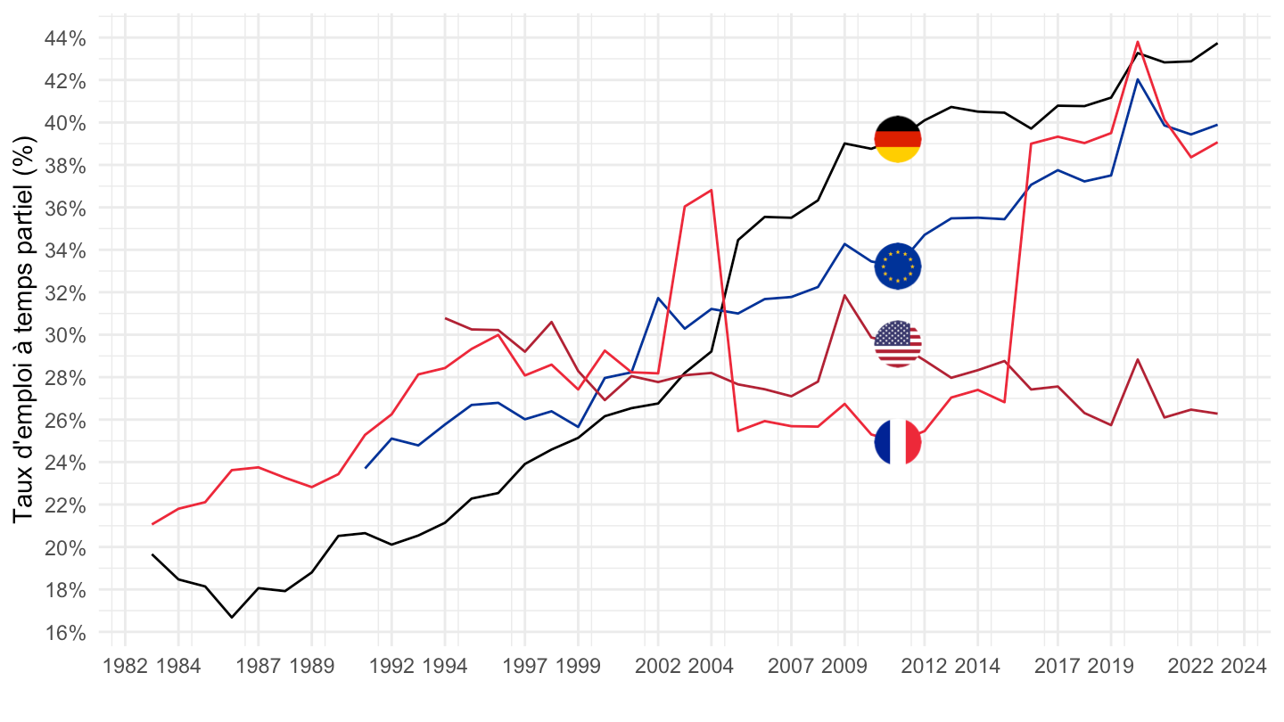
1999-
Code
SL.TLF.PART.ZS %>%
  right_join(iso2c, by = "iso2c") %>%
  filter(iso2c %in% c("US", "XC", "FR", "DE")) %>%
  year_to_date %>%
  mutate(value = value/100) %>%
  filter(date >= as.Date("1999-01-01")) %>%
  mutate(Iso2c = ifelse(iso2c == "XC", "Europe", Iso2c)) %>%
  left_join(colors, by = c("Iso2c" = "country")) %>%
  mutate(color = ifelse(iso2c == "US", color2, color)) %>%
  ggplot(.) + theme_minimal() + scale_color_identity() + xlab("") +
  ylab("Taux d'emploi à temps partiel (%)") +
  geom_line(aes(x = date, y = value, color = color)) + add_4flags +
  scale_x_date(breaks = c(seq(1999, 2100, 5), seq(1997, 2100, 5)) %>% paste0("-01-01") %>% as.Date,
               labels = date_format("%Y")) +
  scale_y_continuous(breaks = 0.01*seq(0, 100, 2),
                     labels = scales::percent_format(accuracy = 1))