| source | dataset | Title | .html | .rData |
|---|---|---|---|---|
| wdi | NE.RSB.GNFS.ZS | External balance on goods and services (% of GDP) | 2026-07-04 | 2026-06-20 |
| wdi | BN.CAB.XOKA.GD.ZS | Current account balance (% of GDP) | 2026-07-04 | 2026-06-20 |
Current account balance (% of GDP)
Data - WDI
Info
Data on main macro
| source | dataset | Title | .html | .rData |
|---|---|---|---|---|
| eurostat | nama_10_a10 | Gross value added and income by A*10 industry breakdowns | 2026-06-20 | 2026-04-26 |
| eurostat | nama_10_a10_e | Employment by A*10 industry breakdowns | 2026-06-20 | 2026-04-26 |
| eurostat | nama_10_gdp | GDP and main components (output, expenditure and income) | 2026-06-20 | 2026-04-26 |
| eurostat | nama_10_lp_ulc | Labour productivity and unit labour costs | 2026-06-20 | 2026-04-26 |
| eurostat | namq_10_a10 | Gross value added and income A*10 industry breakdowns | 2026-06-03 | 2026-06-03 |
| eurostat | namq_10_a10_e | Employment A*10 industry breakdowns | 2025-05-24 | 2026-04-26 |
| eurostat | namq_10_gdp | GDP and main components (output, expenditure and income) | 2025-10-27 | 2026-04-26 |
| eurostat | namq_10_lp_ulc | Labour productivity and unit labour costs | 2026-06-21 | 2026-04-26 |
| eurostat | namq_10_pc | Main GDP aggregates per capita | 2026-03-24 | 2026-04-26 |
| eurostat | nasa_10_nf_tr | Non-financial transactions | 2026-06-21 | 2026-04-26 |
| eurostat | nasq_10_nf_tr | Non-financial transactions | 2026-06-21 | 2026-04-26 |
| fred | gdp | Gross Domestic Product | 2026-07-04 | 2026-07-04 |
| oecd | QNA | Quarterly National Accounts | 2026-06-21 | 2026-06-19 |
| oecd | SNA_TABLE1 | Gross domestic product (GDP) | 2026-06-21 | 2025-05-24 |
| oecd | SNA_TABLE14A | Non-financial accounts by sectors | 2026-06-21 | 2024-06-30 |
| oecd | SNA_TABLE2 | Disposable income and net lending - net borrowing | 2024-07-01 | 2024-04-11 |
| oecd | SNA_TABLE6A | Value added and its components by activity, ISIC rev4 | 2024-07-01 | 2024-06-30 |
| wdi | NE.RSB.GNFS.ZS | External balance on goods and services (% of GDP) | 2026-07-04 | 2026-06-20 |
| wdi | NY.GDP.MKTP.CD | NA | NA | NA |
| wdi | NY.GDP.MKTP.PP.CD | GDP, PPP (current international D) | 2026-07-04 | 2026-06-20 |
| wdi | NY.GDP.PCAP.CD | GDP per capita (current USD) | 2026-07-04 | 2026-06-20 |
| wdi | NY.GDP.PCAP.KD | GDP per capita (constant 2015 USD) | 2026-07-04 | 2026-06-20 |
| wdi | NY.GDP.PCAP.PP.CD | GDP per capita, PPP (current international D) | 2026-02-23 | 2026-06-20 |
| wdi | NY.GDP.PCAP.PP.KD | GDP per capita, PPP (constant 2011 international D) | 2026-07-04 | 2026-06-20 |
LAST_COMPILE
| LAST_COMPILE |
|---|
| 2026-07-04 |
Last
Code
BN.CAB.XOKA.GD.ZS %>%
  group_by(year) %>%
  summarise(Nobs = n()) %>%
  arrange(desc(year)) %>%
  head(1) %>%
print_table_conditional()| year | Nobs |
|---|---|
| 2024 | 162 |
Frugal Four
Code
BN.CAB.XOKA.GD.ZS %>%
  year_to_date %>%
  filter(iso2c %in% c("SE", "AT", "NL","DK")) %>%
  left_join(iso2c, by = "iso2c") %>%
  left_join(colors, by = c("Iso2c" = "country")) %>%
  mutate(value = value/100) %>%
  ggplot(.) +
  geom_line(aes(x = date, y = value, color = color)) +
  theme_minimal() + scale_color_identity() + add_4flags +
  scale_x_date(breaks = seq(1950, 2100, 5) %>% paste0("-01-01") %>% as.Date,
               labels = date_format("%Y")) +
  scale_y_continuous(breaks = 0.01*seq(-60, 60, 2),
                     labels = scales::percent_format(accuracy = 1)) +
  xlab("") + ylab("Current Account (% of GDP)") +
  geom_hline(yintercept = 0, linetype = "dashed",  color = "black")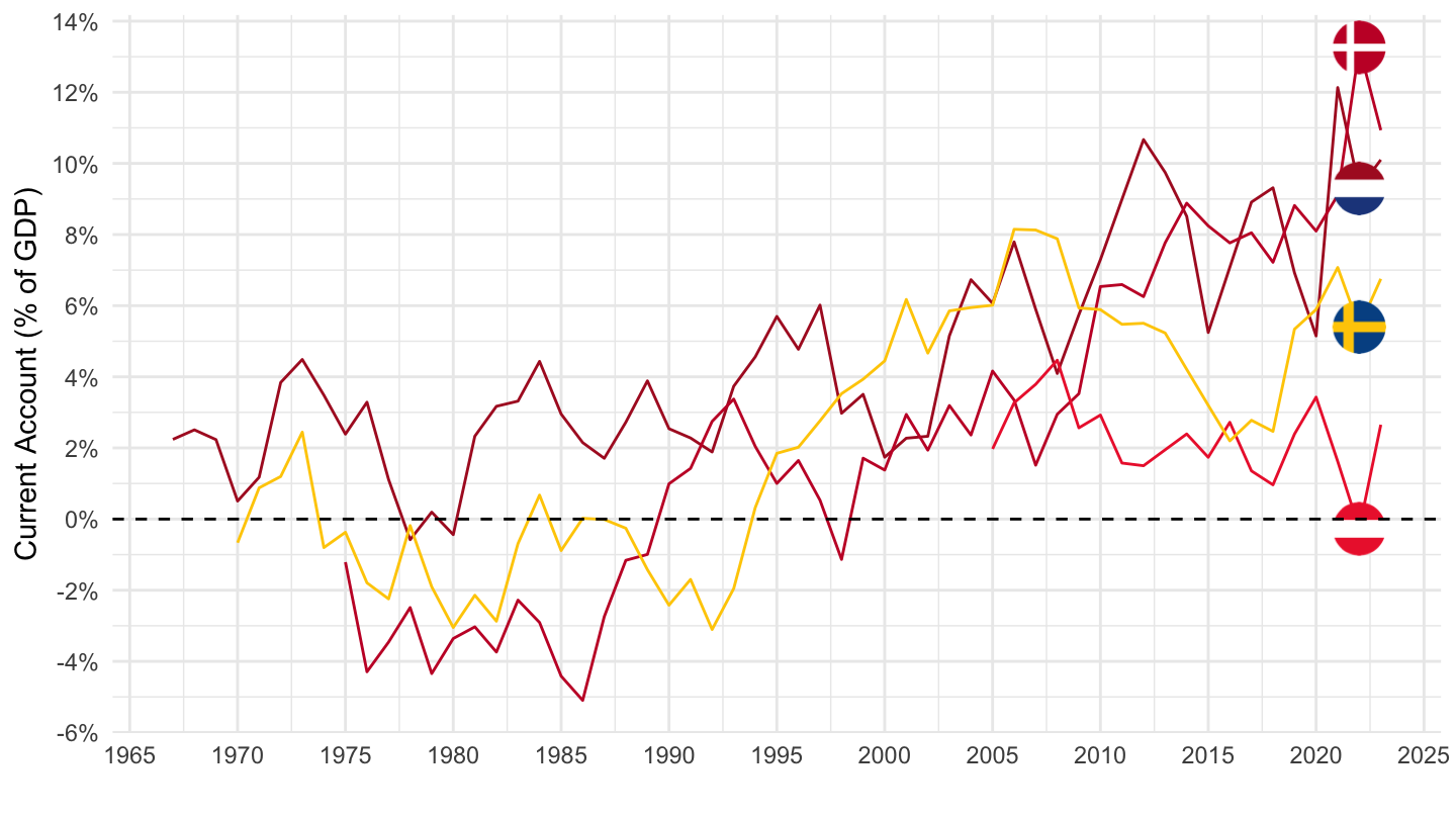
Nobs - Javascript
Code
BN.CAB.XOKA.GD.ZS %>%
  left_join(iso2c, by = "iso2c") %>%
  group_by(iso2c, Iso2c) %>%
  mutate(value = round(value, 2)) %>%
  summarise(Nobs = n(),
            `Year 1` = first(year),
            `CA 1 (%)` = first(value),
            `Year 2` = last(year),
            `CA 2 (%)` = last(value)) %>%
  arrange(-Nobs) %>%
  {if (is_html_output()) datatable(., filter = 'top', rownames = F) else .}
Crises in Emerging Markets (Source: Vegh (2013))
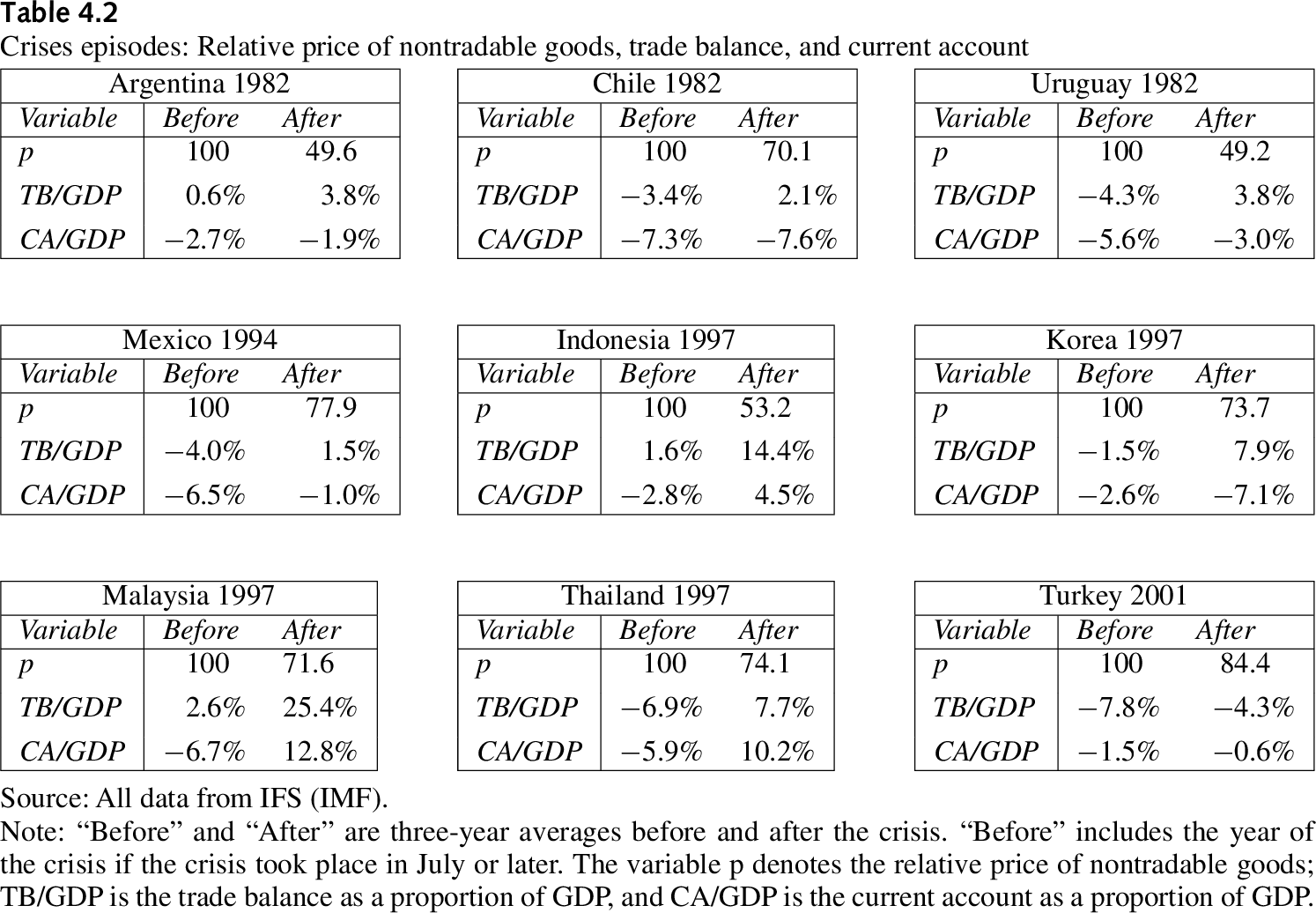
1982: Southern Cone - Argentina, Chile, Uruguay
Code
BN.CAB.XOKA.GD.ZS %>%
  year_to_date %>%
  filter(iso2c %in% c("AR", "CL", "UY"),
            date <= as.Date("1986-01-01")) %>%
  left_join(iso2c, by = "iso2c") %>%
  left_join(colors, by = c("Iso2c" = "country")) %>%
  mutate(value = value/100) %>%
  ggplot(.) +
  geom_line(aes(x = date, y = value, color = color)) +
  theme_minimal() + scale_color_identity() + add_3flags +
  scale_x_date(breaks = seq(1950, 2100, 1) %>% paste0("-01-01") %>% as.Date,
               labels = date_format("%Y")) +
  scale_y_continuous(breaks = 0.01*seq(-60, 60, 2),
                     labels = scales::percent_format(accuracy = 1)) +
  xlab("") + ylab("Current Account (% of GDP)") +
  geom_hline(yintercept = 0, linetype = "dashed",  color = "black")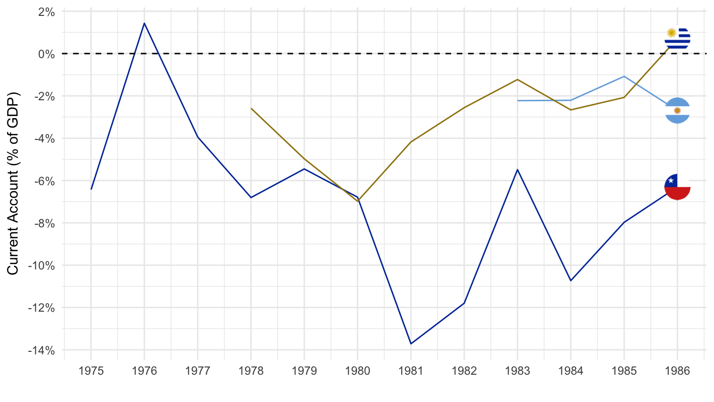
1994: Mexico
Code
BN.CAB.XOKA.GD.ZS %>%
  year_to_date %>%
  filter(iso2c %in% c("MX"),
         date >= as.Date("1989-01-01")) %>%
  left_join(iso2c, by = "iso2c") %>%
  left_join(colors, by = c("Iso2c" = "country")) %>%
  mutate(value = value/100) %>%
  ggplot(.) +
  geom_line(aes(x = date, y = value, color = color)) +
  theme_minimal() + scale_color_identity() +
  scale_x_date(breaks = seq(1950, 2100, 1) %>% paste0("-01-01") %>% as.Date,
               labels = date_format("%Y")) +
  scale_y_continuous(breaks = 0.01*seq(-60, 60, 1),
                     labels = scales::percent_format(accuracy = 1)) +
  xlab("") + ylab("Current Account (% of GDP)") +
  geom_hline(yintercept = 0, linetype = "dashed",  color = "black")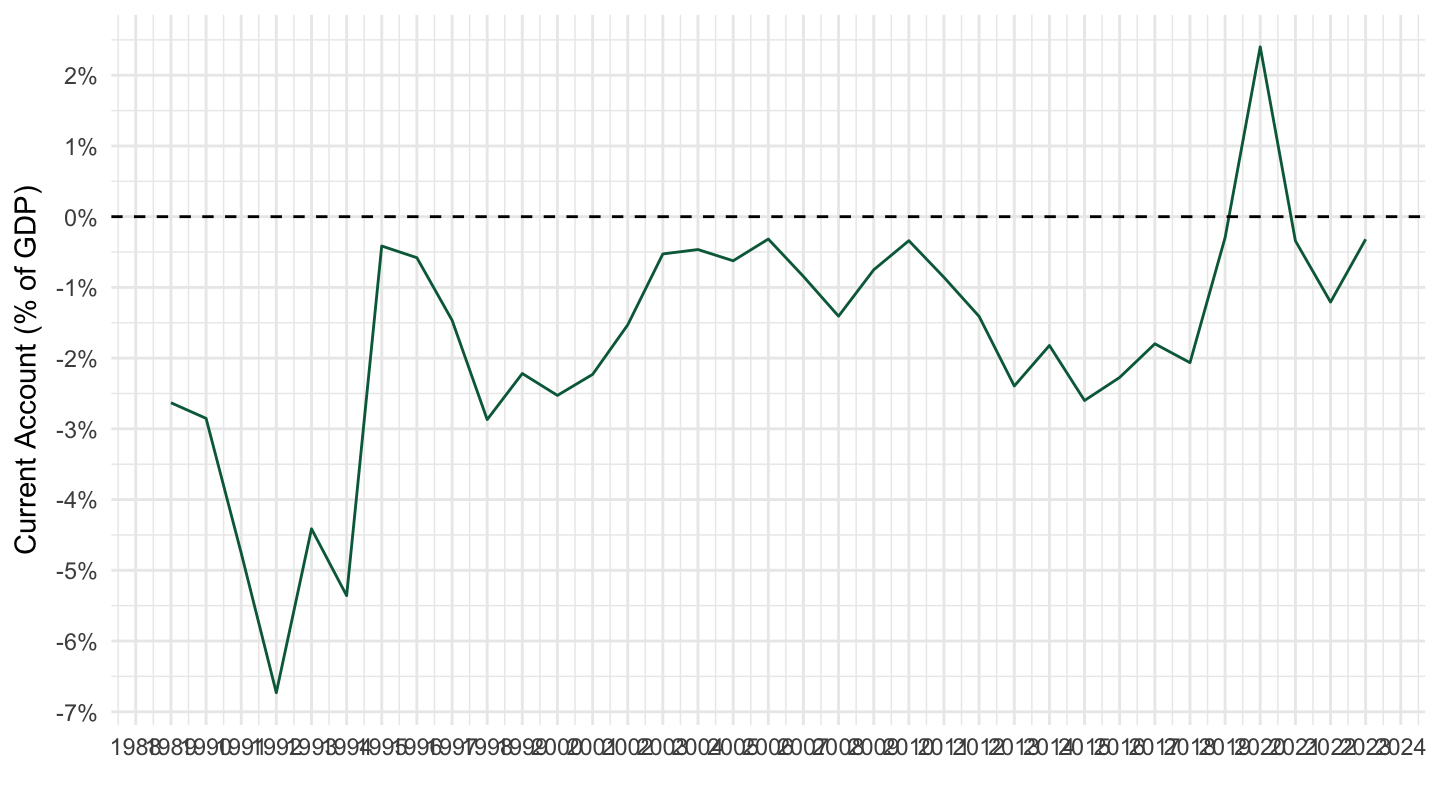
1995: Hungary
Code
BN.CAB.XOKA.GD.ZS %>%
  year_to_date %>%
  filter(iso2c %in% c("HU"),
         date >= as.Date("1995-01-01")) %>%
  left_join(iso2c, by = "iso2c") %>%
  ggplot(.) +
  geom_line(aes(x = date, y = value/100)) +
  theme_minimal() + scale_color_manual(values = viridis(5)[1:4]) +
  theme(legend.title = element_blank(),
        legend.position = c(0.2, 0.8)) +
  scale_x_date(breaks = seq(1950, 2100, 1) %>% paste0("-01-01") %>% as.Date,
               labels = date_format("%Y")) +
  scale_y_continuous(breaks = 0.01*seq(-60, 60, 1),
                     labels = scales::percent_format(accuracy = 1)) +
  xlab("") + ylab("Current Account (% of GDP)") +
  geom_hline(yintercept = 0, linetype = "dashed",  color = "black")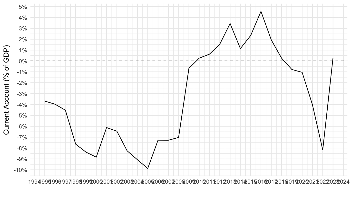
1997: Russia
Code
BN.CAB.XOKA.GD.ZS %>%
  year_to_date %>%
  filter(iso2c %in% c("RU"),
         date <= as.Date("2002-01-01"),
         date >= as.Date("1980-01-01")) %>%
  left_join(iso2c, by = "iso2c") %>%
  ggplot(.) +
  geom_line(aes(x = date, y = value/100, color = Iso2c, linetype = Iso2c)) +
  theme_minimal() + scale_color_manual(values = viridis(5)[1:4]) +
  theme(legend.title = element_blank(),
        legend.position = c(0.2, 0.8)) +
  scale_x_date(breaks = seq(1950, 2100, 1) %>% paste0("-01-01") %>% as.Date,
               labels = date_format("%Y")) +
  scale_y_continuous(breaks = 0.01*seq(-60, 60, 2),
                     labels = scales::percent_format(accuracy = 1)) +
  xlab("") + ylab("Current Account (% of GDP)") +
  geom_hline(yintercept = 0, linetype = "dashed",  color = "black")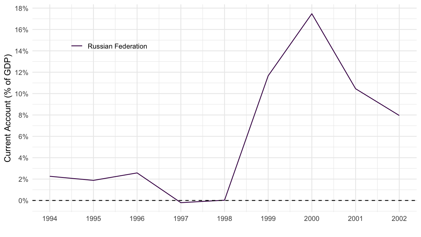
1997: East Asia - Indonesia, Korea, Malaysia, Thailand
Code
BN.CAB.XOKA.GD.ZS %>%
  year_to_date %>%
  filter(iso2c %in% c("ID", "KR", "MY", "TH"),
         date <= as.Date("2002-01-01"),
         date >= as.Date("1992-01-01")) %>%
  left_join(iso2c, by = "iso2c") %>%
  left_join(colors, by = c("Iso2c" = "country")) %>%
  mutate(value = value/100,
         Iso2c = ifelse(iso2c == "KR", "South Korea", Iso2c)) %>%
  ggplot(.) +
  geom_line(aes(x = date, y = value, color = color)) +
  theme_minimal() + scale_color_identity() + add_4flags +
  scale_x_date(breaks = seq(1950, 2100, 1) %>% paste0("-01-01") %>% as.Date,
               labels = date_format("%Y")) +
  scale_y_continuous(breaks = 0.01*seq(-60, 60, 2),
                     labels = scales::percent_format(accuracy = 1)) +
  xlab("") + ylab("Current Account (% of GDP)") +
  geom_hline(yintercept = 0, linetype = "dashed",  color = "black")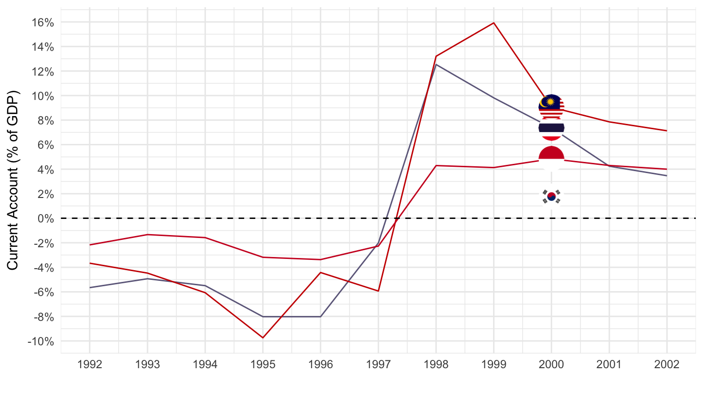
2001: Turkey
Code
BN.CAB.XOKA.GD.ZS %>%
  year_to_date %>%
  filter(iso2c %in% c("TR"),
         date <= as.Date("2006-01-01"),
         date >= as.Date("1996-01-01")) %>%
  left_join(iso2c, by = "iso2c") %>%
  ggplot(.) +
  geom_line(aes(x = date, y = value/100)) +
  theme_minimal() + scale_color_manual(values = viridis(5)[1:4]) +
  theme(legend.title = element_blank(),
        legend.position = c(0.2, 0.8)) +
  scale_x_date(breaks = seq(1950, 2100, 1) %>% paste0("-01-01") %>% as.Date,
               labels = date_format("%Y")) +
  scale_y_continuous(breaks = 0.01*seq(-60, 60, 1),
                     labels = scales::percent_format(accuracy = 1)) +
  xlab("") + ylab("Current Account (% of GDP)") +
  geom_hline(yintercept = 0, linetype = "dashed",  color = "black")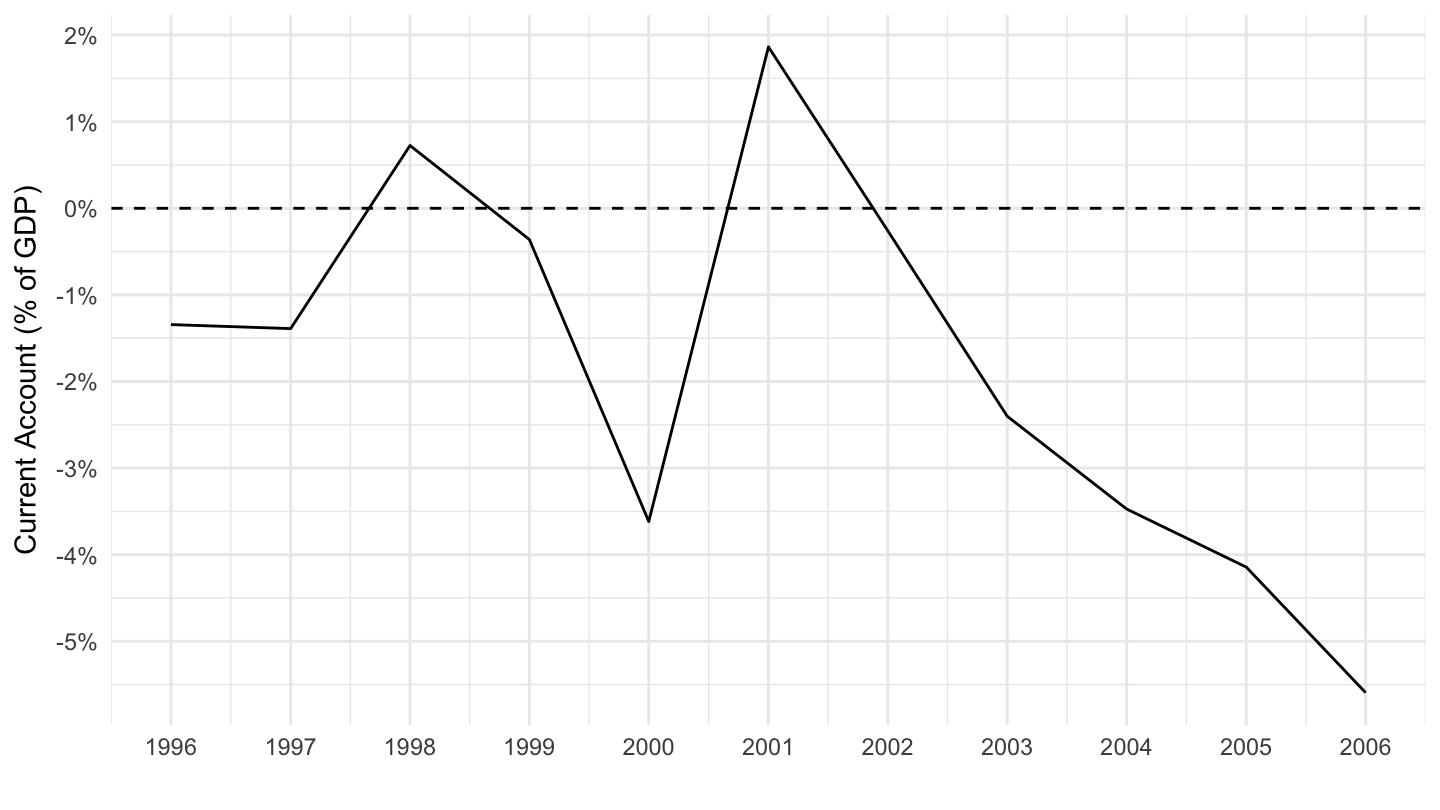
2002: Uruguay Crisis
Code
BN.CAB.XOKA.GD.ZS %>%
  year_to_date %>%
  filter(iso2c %in% c("UY"),
         date <= as.Date("2006-01-01"),
         date >= as.Date("1996-01-01")) %>%
  left_join(iso2c, by = "iso2c") %>%
  ggplot(.) +
  geom_line(aes(x = date, y = value/100)) +
  theme_minimal() + scale_color_manual(values = viridis(5)[1:4]) +
  theme(legend.title = element_blank(),
        legend.position = c(0.2, 0.8)) +
  scale_x_date(breaks = seq(1950, 2100, 1) %>% paste0("-01-01") %>% as.Date,
               labels = date_format("%Y")) +
  scale_y_continuous(breaks = 0.01*seq(-60, 60, 1),
                     labels = scales::percent_format(accuracy = 1)) +
  xlab("") + ylab("Current Account (% of GDP)") +
  geom_hline(yintercept = 0, linetype = "dashed",  color = "black")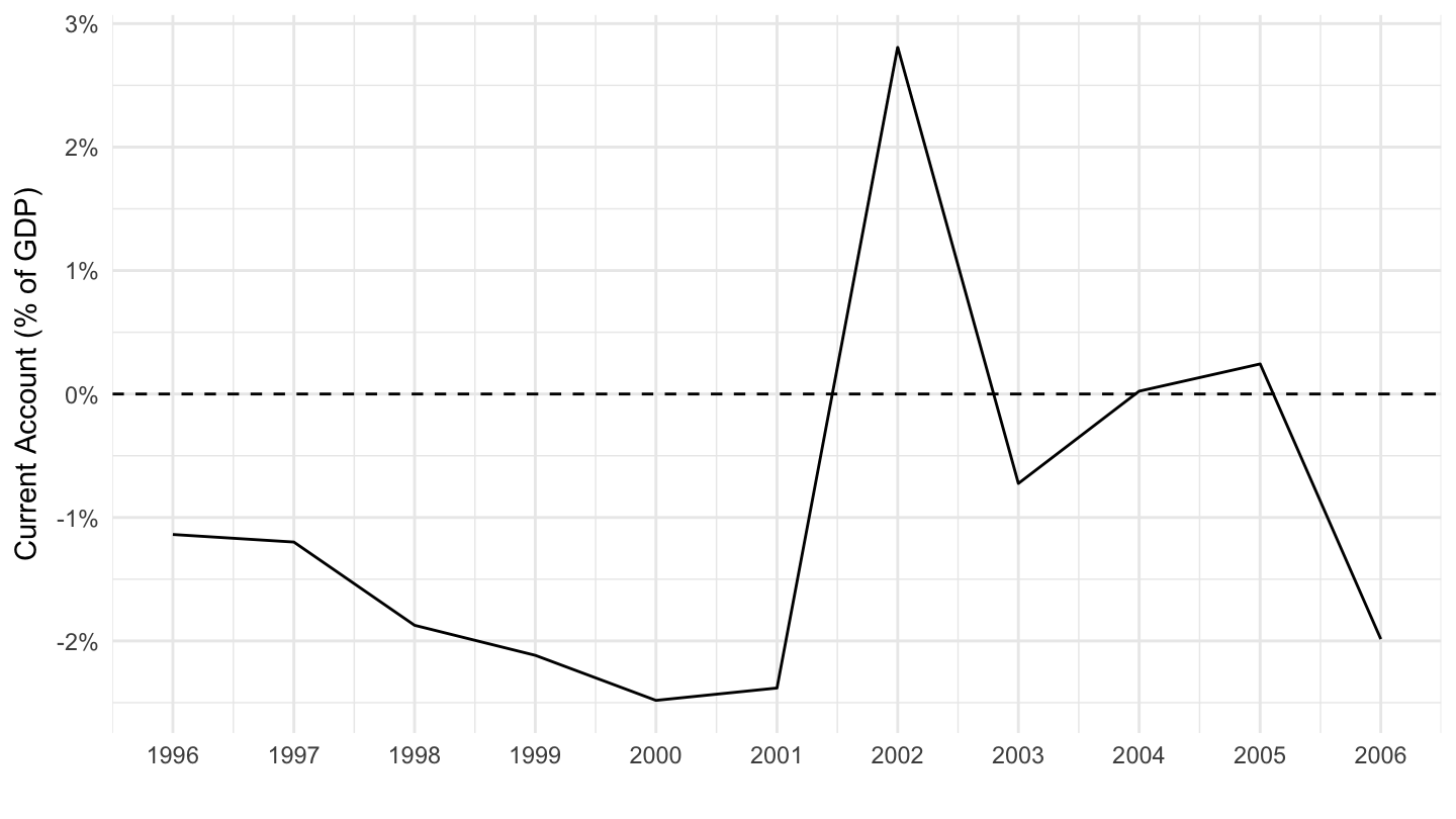
Israel
All
Code
BN.CAB.XOKA.GD.ZS %>%
  year_to_date %>%
  filter(iso2c %in% c("IL")) %>%
  left_join(iso2c, by = "iso2c") %>%
  ggplot(.) +
  geom_line(aes(x = date, y = value/100)) +
  theme_minimal() + scale_color_manual(values = viridis(5)[1:4]) +
  theme(legend.title = element_blank(),
        legend.position = c(0.2, 0.8)) +
  scale_x_date(breaks = seq(1950, 2100, 2) %>% paste0("-01-01") %>% as.Date,
               labels = date_format("%Y")) +
  scale_y_continuous(breaks = 0.01*seq(-60, 60, 2),
                     labels = scales::percent_format(accuracy = 1)) +
  xlab("") + ylab("Current Account (% of GDP)") +
  geom_hline(yintercept = 0, linetype = "dashed",  color = "black")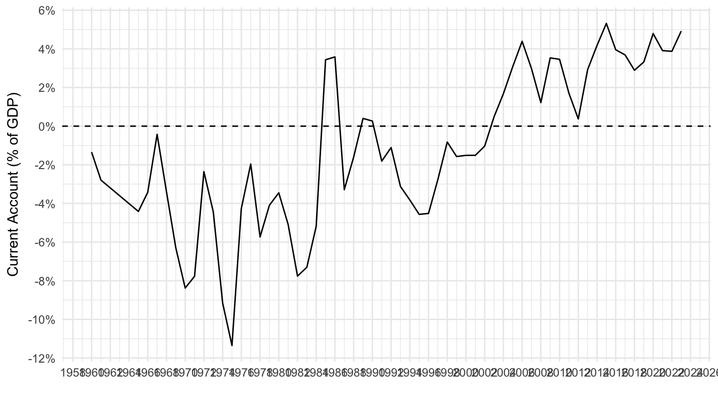
2000-
Code
BN.CAB.XOKA.GD.ZS %>%
  year_to_date %>%
  filter(iso2c %in% c("IL"),
         date >= as.Date("2000-01-01")) %>%
  left_join(iso2c, by = "iso2c") %>%
  ggplot(.) +
  geom_line(aes(x = date, y = value/100)) +
  theme_minimal() + scale_color_manual(values = viridis(5)[1:4]) +
  theme(legend.title = element_blank(),
        legend.position = c(0.2, 0.8)) +
  scale_x_date(breaks = seq(1950, 2100, 2) %>% paste0("-01-01") %>% as.Date,
               labels = date_format("%Y")) +
  scale_y_continuous(breaks = 0.01*seq(-60, 60, 1),
                     labels = scales::percent_format(accuracy = 1)) +
  xlab("") + ylab("Current Account (% of GDP)") +
  geom_hline(yintercept = 0, linetype = "dashed",  color = "black")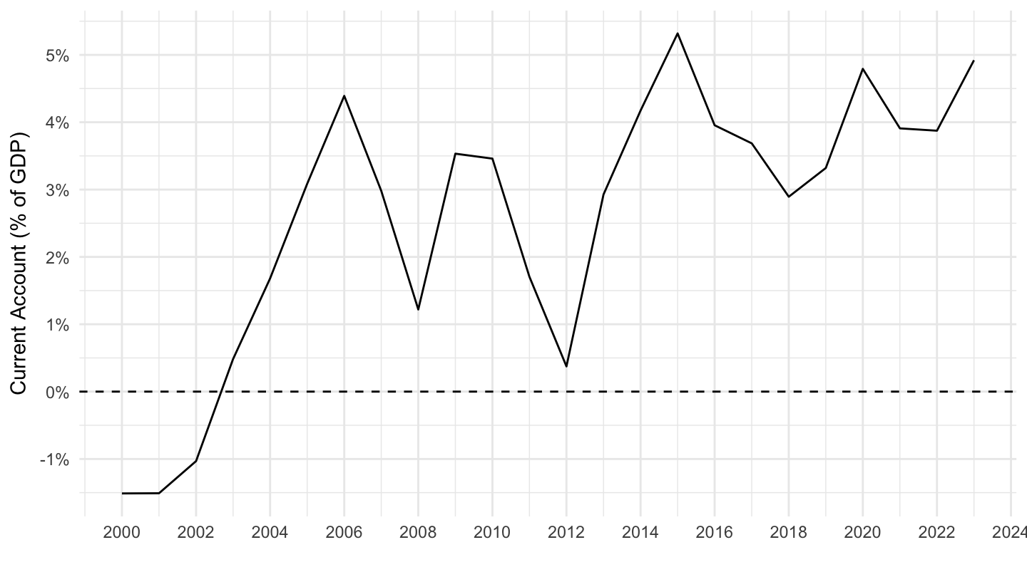
2010-
Code
BN.CAB.XOKA.GD.ZS %>%
  year_to_date %>%
  filter(iso2c %in% c("IL"),
         date >= as.Date("2010-01-01")) %>%
  left_join(iso2c, by = "iso2c") %>%
  ggplot(.) +
  geom_line(aes(x = date, y = value/100)) +
  theme_minimal() + scale_color_manual(values = viridis(5)[1:4]) +
  theme(legend.title = element_blank(),
        legend.position = c(0.2, 0.8)) +
  scale_x_date(breaks = seq(1950, 2100, 1) %>% paste0("-01-01") %>% as.Date,
               labels = date_format("%Y")) +
  scale_y_continuous(breaks = 0.01*seq(-60, 60, 1),
                     labels = scales::percent_format(accuracy = 1)) +
  xlab("") + ylab("Current Account (% of GDP)") +
  geom_hline(yintercept = 0, linetype = "dashed",  color = "black")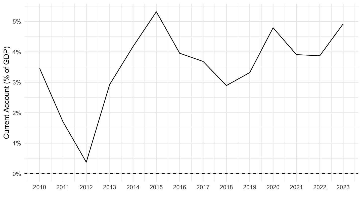
Lebanon
Code
BN.CAB.XOKA.GD.ZS %>%
  year_to_date %>%
  filter(iso2c %in% c("LB")) %>%
  left_join(iso2c, by = "iso2c") %>%
  ggplot(.) +
  geom_line(aes(x = date, y = value/100)) +
  theme_minimal() + scale_color_manual(values = viridis(5)[1:4]) +
  theme(legend.title = element_blank(),
        legend.position = c(0.2, 0.8)) +
  scale_x_date(breaks = seq(1950, 2100, 2) %>% paste0("-01-01") %>% as.Date,
               labels = date_format("%Y")) +
  scale_y_continuous(breaks = 0.01*seq(-60, 60, 2),
                     labels = scales::percent_format(accuracy = 1)) +
  xlab("") + ylab("Current Account (% of GDP)") +
  geom_hline(yintercept = 0, linetype = "dashed",  color = "black")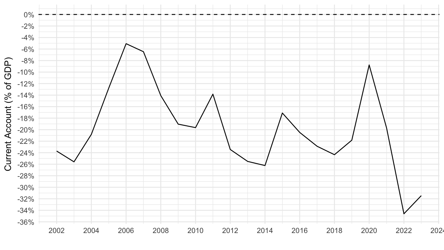
Vietnam
Code
BN.CAB.XOKA.GD.ZS %>%
  year_to_date %>%
  filter(iso2c %in% c("VN"),
         date >= as.Date("1995-01-01")) %>%
  left_join(iso2c, by = "iso2c") %>%
  ggplot(.) +
  geom_line(aes(x = date, y = value/100)) +
  theme_minimal() + scale_color_manual(values = viridis(5)[1:4]) +
  theme(legend.title = element_blank(),
        legend.position = c(0.2, 0.8)) +
  scale_x_date(breaks = seq(1950, 2100, 2) %>% paste0("-01-01") %>% as.Date,
               labels = date_format("%Y")) +
  scale_y_continuous(breaks = 0.01*seq(-60, 60, 2),
                     labels = scales::percent_format(accuracy = 1)) +
  xlab("") + ylab("Current Account (% of GDP)") +
  geom_hline(yintercept = 0, linetype = "dashed",  color = "black")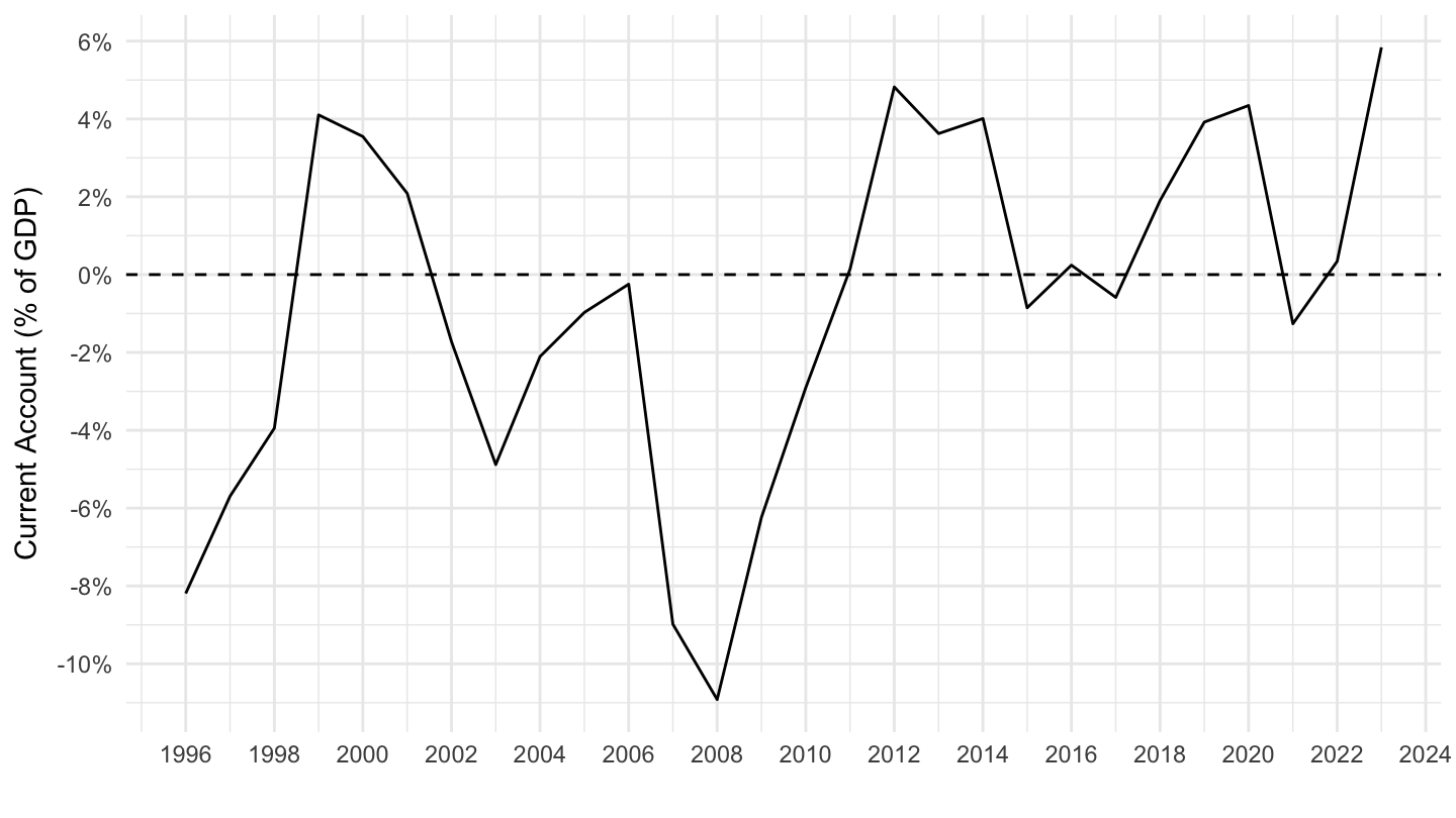
Russia
Code
BN.CAB.XOKA.GD.ZS %>%
  year_to_date %>%
  filter(iso2c %in% c("RU"),
         date >= as.Date("1995-01-01")) %>%
  left_join(iso2c, by = "iso2c") %>%
  ggplot(.) +
  geom_line(aes(x = date, y = value/100)) +
  theme_minimal() + scale_color_manual(values = viridis(5)[1:4]) +
  theme(legend.title = element_blank(),
        legend.position = c(0.2, 0.8)) +
  scale_x_date(breaks = seq(1950, 2100, 2) %>% paste0("-01-01") %>% as.Date,
               labels = date_format("%Y")) +
  scale_y_continuous(breaks = 0.01*seq(-60, 60, 2),
                     labels = scales::percent_format(accuracy = 1)) +
  xlab("") + ylab("Current Account (% of GDP)") +
  geom_hline(yintercept = 0, linetype = "dashed",  color = "black")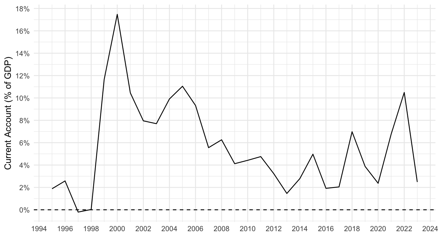
Iceland
Code
BN.CAB.XOKA.GD.ZS %>%
  year_to_date %>%
  filter(iso2c %in% c("IS"),
         date >= as.Date("1995-01-01")) %>%
  left_join(iso2c, by = "iso2c") %>%
  ggplot(.) +
  geom_line(aes(x = date, y = value/100)) +
  theme_minimal() + scale_color_manual(values = viridis(5)[1:4]) +
  theme(legend.title = element_blank(),
        legend.position = c(0.2, 0.8)) +
  scale_x_date(breaks = seq(1950, 2100, 2) %>% paste0("-01-01") %>% as.Date,
               labels = date_format("%Y")) +
  scale_y_continuous(breaks = 0.01*seq(-60, 60, 2),
                     labels = scales::percent_format(accuracy = 1)) +
  xlab("") + ylab("Current Account (% of GDP)") +
  geom_hline(yintercept = 0, linetype = "dashed",  color = "black")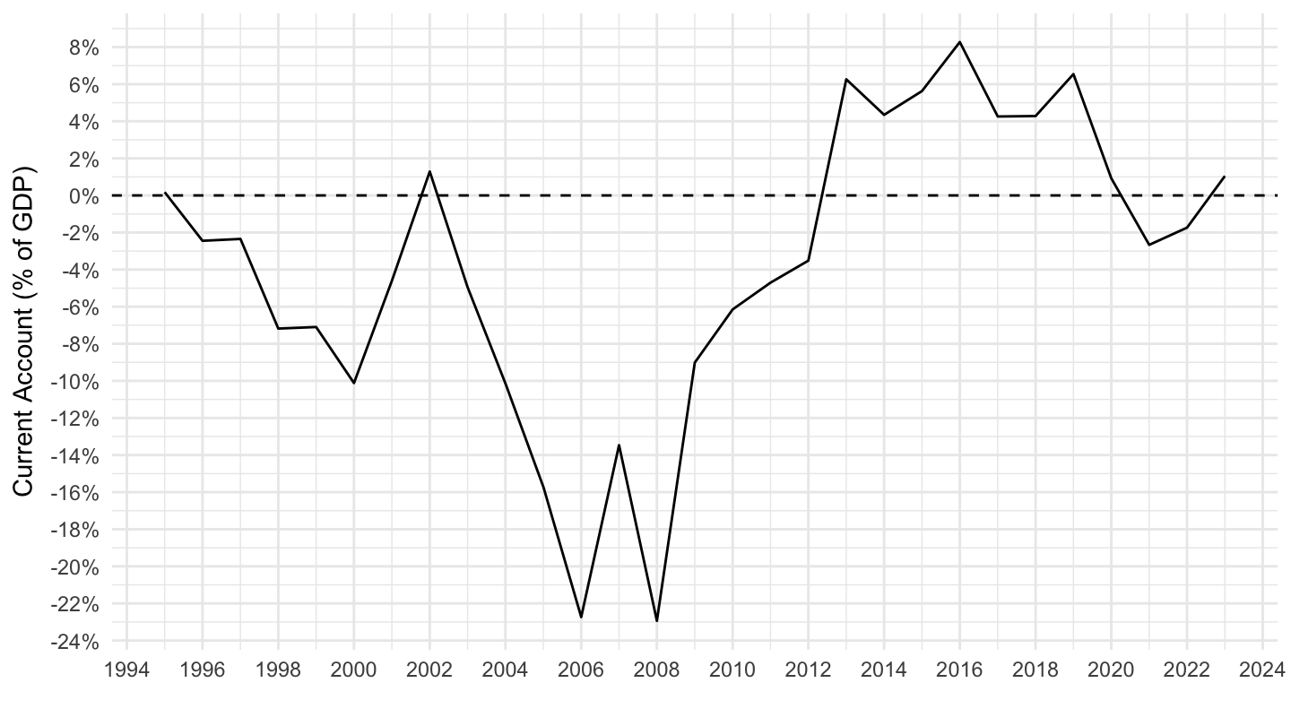
Lebanon, Greece
French
Code
BN.CAB.XOKA.GD.ZS %>%
  filter(iso2c %in% c("LB", "GR")) %>%
  year_to_date %>%
  left_join(iso2c, by = "iso2c") %>%
  left_join(colors, by = c("Iso2c" = "country")) %>%
  mutate(value = value/100) %>%
  ggplot(.) +
  geom_line(aes(x = date, y = value, color = color)) +
  theme_minimal() + scale_color_identity() + add_2flags +
  scale_x_date(breaks = seq(1950, 2100, 5) %>% paste0("-01-01") %>% as.Date,
               labels = date_format("%Y")) +
  scale_y_continuous(breaks = 0.01*seq(-60, 60, 2),
                     labels = scales::percent_format(accuracy = 1)) +
  xlab("") + ylab("Current Account (% of GDP)") +
  geom_hline(yintercept = 0, linetype = "dashed",  color = "black")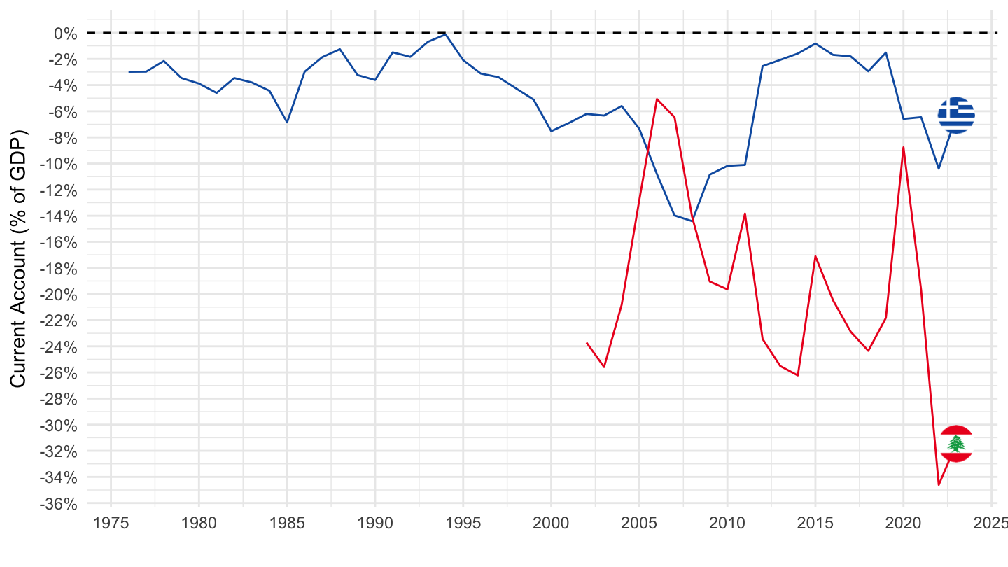
Costa Rica, Philippines
Code
BN.CAB.XOKA.GD.ZS %>%
  filter(iso2c %in% c("CR", "PH")) %>%
  year_to_date %>%
  left_join(iso2c, by = "iso2c") %>%
  left_join(colors, by = c("Iso2c" = "country")) %>%
  mutate(value = value/100) %>%
  ggplot(.) +
  geom_line(aes(x = date, y = value, color = color)) +
  theme_minimal() + scale_color_identity() + add_2flags +
  scale_x_date(breaks = seq(1950, 2100, 5) %>% paste0("-01-01") %>% as.Date,
               labels = date_format("%Y")) +
  scale_y_continuous(breaks = 0.01*seq(-60, 60, 2),
                     labels = scales::percent_format(accuracy = 1)) +
  xlab("") + ylab("Current Account (% of GDP)") +
  geom_hline(yintercept = 0, linetype = "dashed",  color = "black")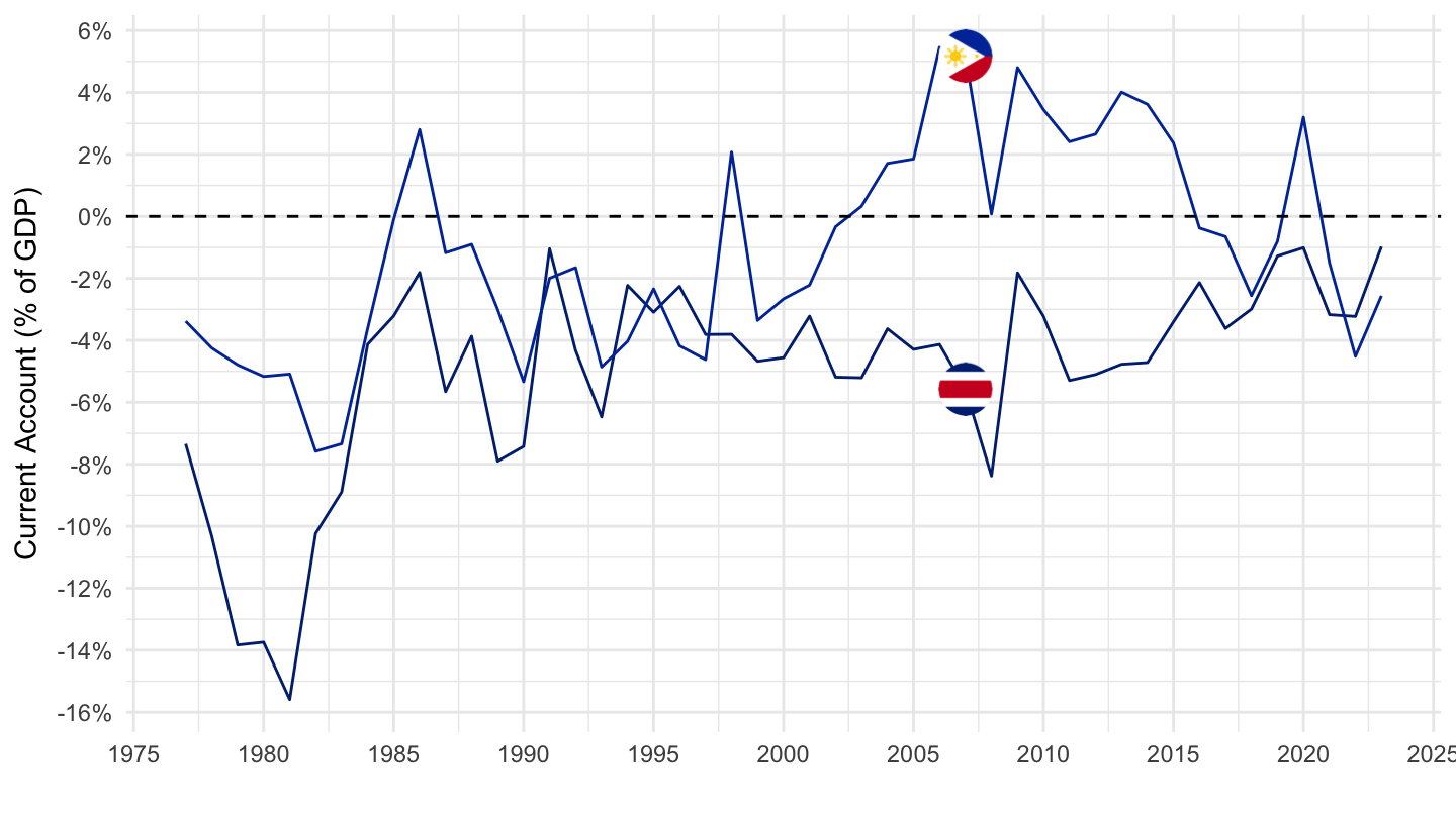
France, Germany, Italy
Code
BN.CAB.XOKA.GD.ZS %>%
  filter(iso2c %in% c("IT", "FR", "DE")) %>%
  year_to_date %>%
  left_join(iso2c, by = "iso2c") %>%
  left_join(colors, by = c("Iso2c" = "country")) %>%
  mutate(value = value/100) %>%
  ggplot(.) +
  geom_line(aes(x = date, y = value, color = color)) +
  theme_minimal() + scale_color_identity() + add_3flags +
  scale_x_date(breaks = seq(1950, 2100, 5) %>% paste0("-01-01") %>% as.Date,
               labels = date_format("%Y")) +
  scale_y_continuous(breaks = 0.01*seq(-60, 60, 1),
                     labels = scales::percent_format(accuracy = 1)) +
  xlab("") + ylab("Current Account (% of GDP)") +
  geom_hline(yintercept = 0, linetype = "dashed",  color = "black")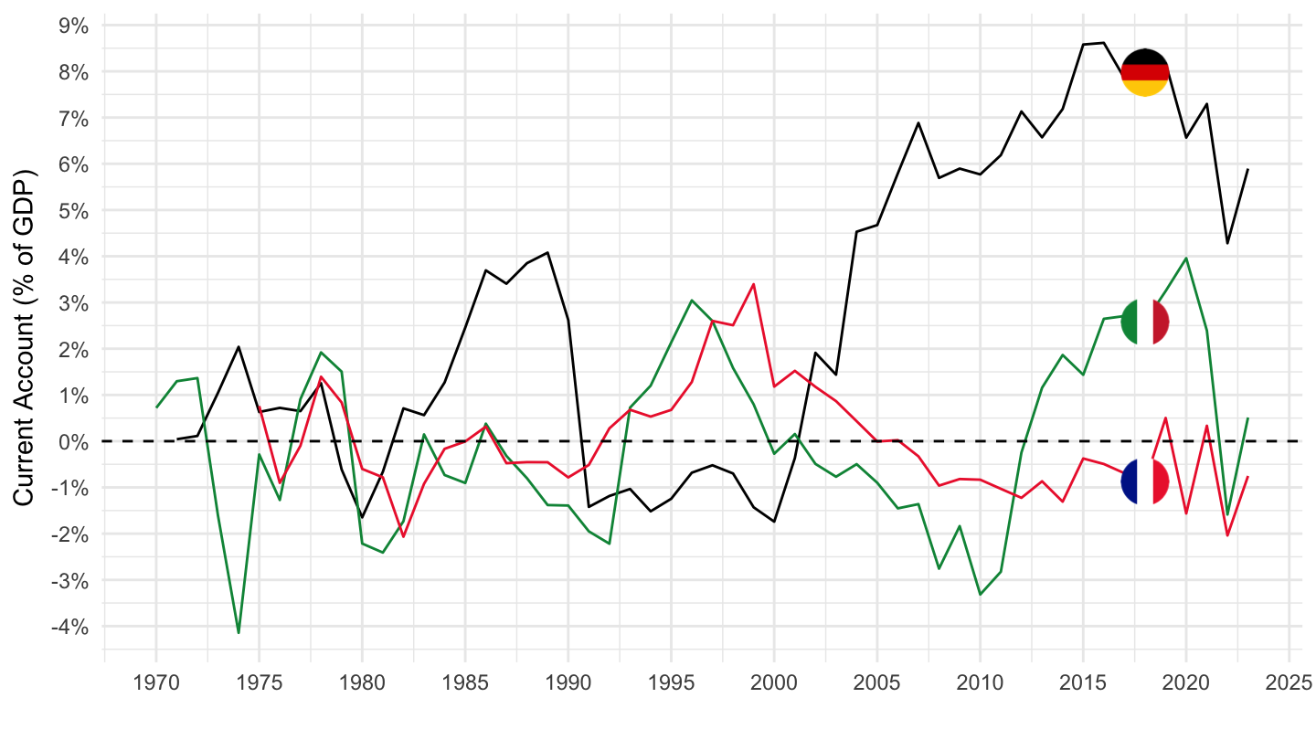
United States, Europe
Code
BN.CAB.XOKA.GD.ZS %>%
  filter(iso2c %in% c("US", "U2")) %>%
  year_to_date %>%
  left_join(iso2c, by = "iso2c") %>%
  left_join(colors, by = c("Iso2c" = "country")) %>%
  mutate(value = value/100,
         Iso2c = ifelse(iso2c == "U2", "Europe", Iso2c)) %>%
  ggplot(.) +
  geom_line(aes(x = date, y = value, color = color)) +
  theme_minimal() + scale_color_identity() + add_2flags +
  scale_x_date(breaks = seq(1950, 2100, 5) %>% paste0("-01-01") %>% as.Date,
               labels = date_format("%Y")) +
  scale_y_continuous(breaks = 0.01*seq(-60, 60, 1),
                     labels = scales::percent_format(accuracy = 1)) +
  xlab("") + ylab("Current Account (% of GDP)") +
  geom_hline(yintercept = 0, linetype = "dashed",  color = "black")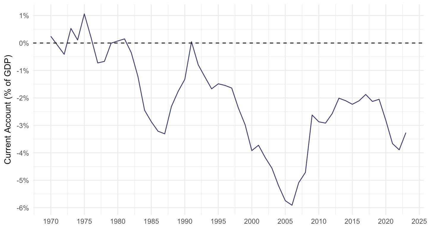
France, Germany, Italy, China
All
Code
BN.CAB.XOKA.GD.ZS %>%
  filter(iso2c %in% c("IT", "FR", "DE", "CN")) %>%
  year_to_date %>%
  left_join(iso2c, by = "iso2c") %>%
  left_join(colors, by = c("Iso2c" = "country")) %>%
  mutate(value = value/100) %>%
  ggplot(.) +
  geom_line(aes(x = date, y = value, color = color)) +
  theme_minimal() + scale_color_identity() + add_4flags +
  scale_x_date(breaks = seq(1950, 2100, 5) %>% paste0("-01-01") %>% as.Date,
               labels = date_format("%Y")) +
  scale_y_continuous(breaks = 0.01*seq(-60, 60, 1),
                     labels = scales::percent_format(accuracy = 1)) +
  xlab("") + ylab("Current Account (% of GDP)") +
  geom_hline(yintercept = 0, linetype = "dashed",  color = "black")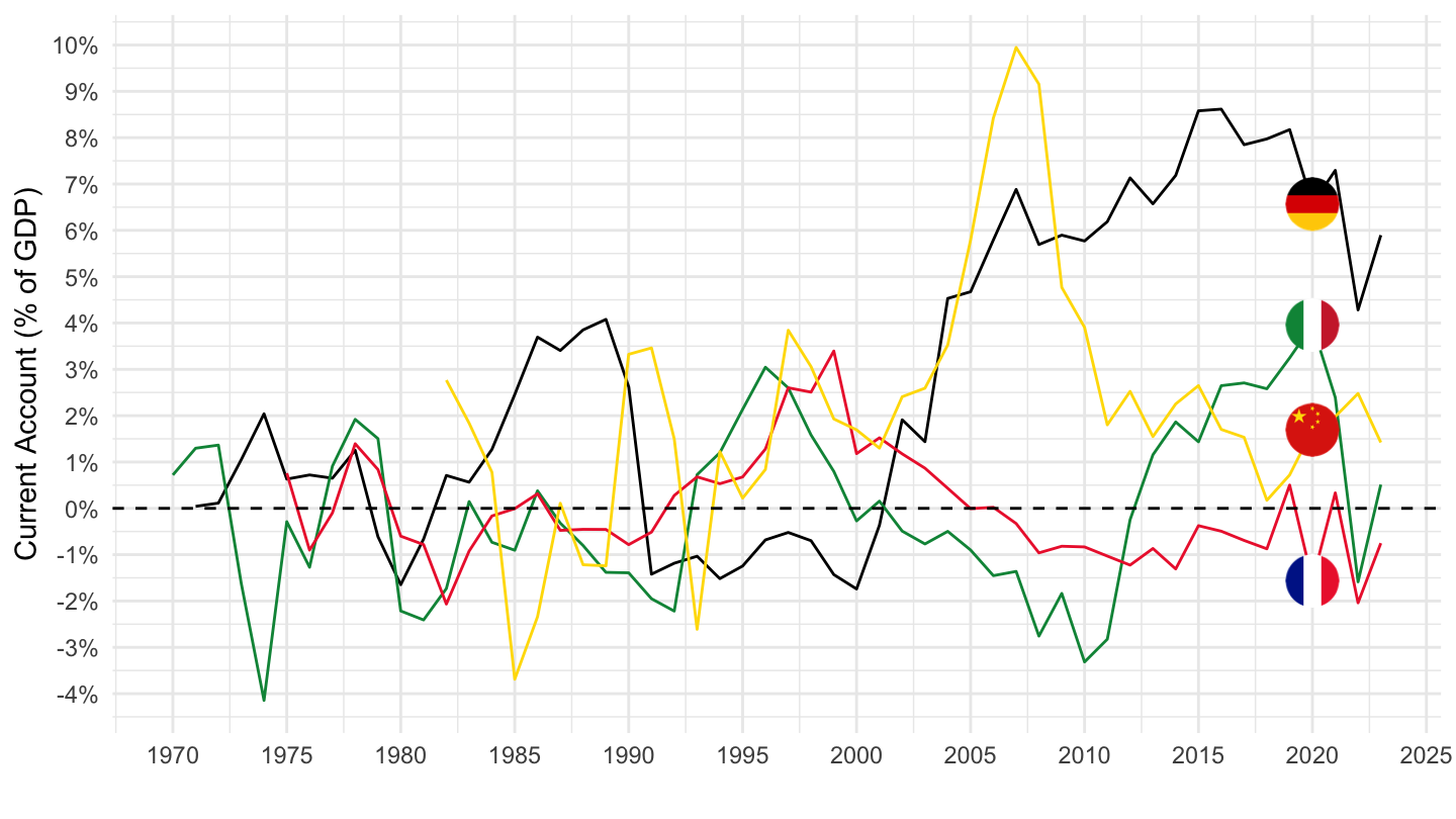
1982-
Code
BN.CAB.XOKA.GD.ZS %>%
  filter(iso2c %in% c("IT", "FR", "DE", "CN")) %>%
  year_to_date %>%
  left_join(iso2c, by = "iso2c") %>%
  left_join(colors, by = c("Iso2c" = "country")) %>%
  mutate(value = value/100) %>%
  filter(date >= as.Date("1982-01-01")) %>%
  ggplot(.) +
  geom_line(aes(x = date, y = value, color = color)) +
  theme_minimal() + scale_color_identity() + add_4flags +
  scale_x_date(breaks = seq(1950, 2100, 5) %>% paste0("-01-01") %>% as.Date,
               labels = date_format("%Y")) +
  scale_y_continuous(breaks = 0.01*seq(-60, 60, 1),
                     labels = scales::percent_format(accuracy = 1)) +
  xlab("") + ylab("Current Account (% of GDP)") +
  geom_hline(yintercept = 0, linetype = "dashed",  color = "black")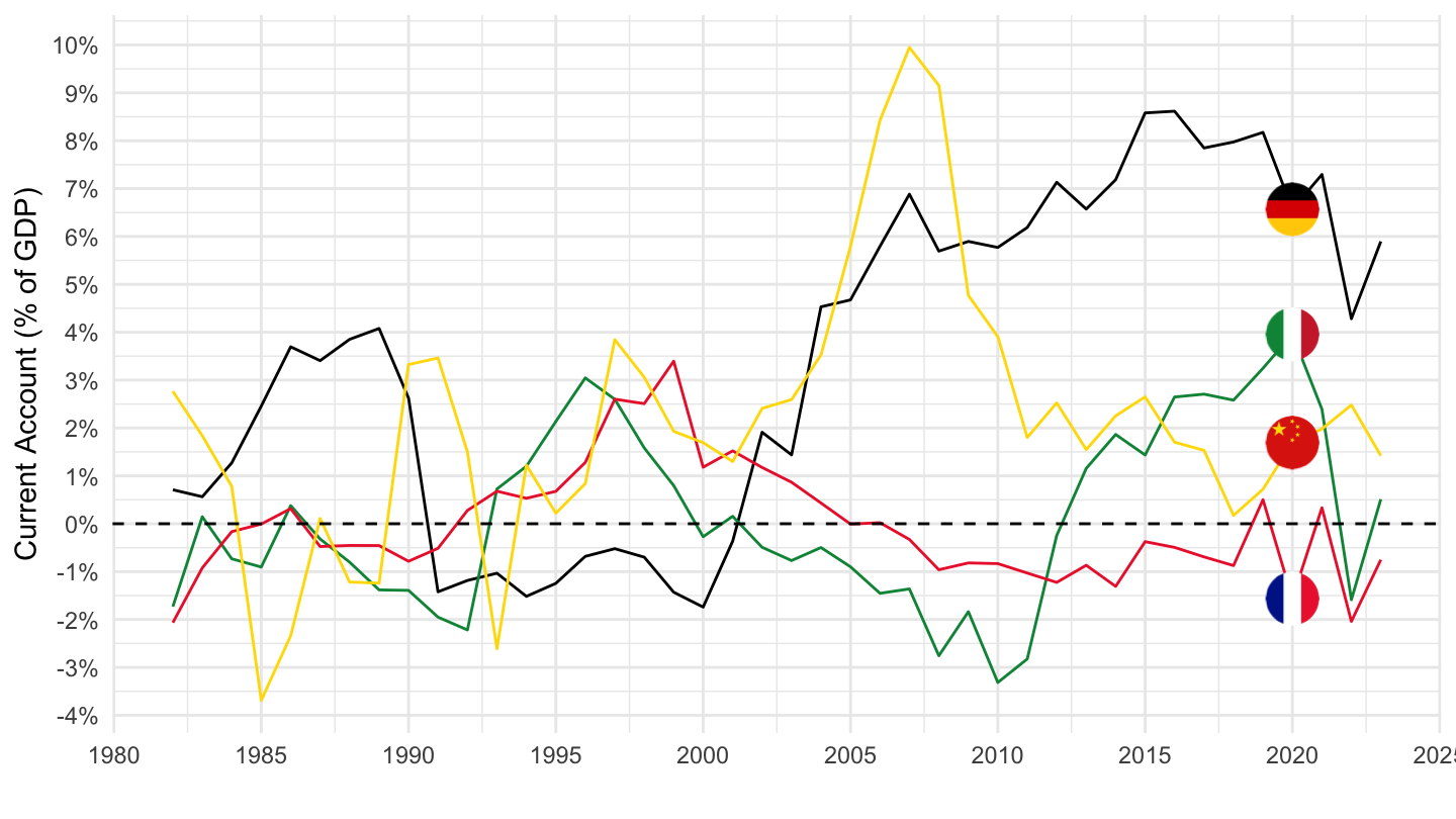
Saudi Arabia, Jordan, Kuwait
Code
BN.CAB.XOKA.GD.ZS %>%
  filter(iso2c %in% c("SA", "JO", "KW")) %>%
  year_to_date %>%
  left_join(iso2c, by = "iso2c") %>%
  left_join(colors, by = c("Iso2c" = "country")) %>%
  mutate(color = ifelse(iso2c == "KW", color2, color)) %>%
  mutate(value = value/100) %>%
  ggplot(.) +
  geom_line(aes(x = date, y = value, color = color)) +
  theme_minimal() + scale_color_identity() + add_3flags +
  scale_x_date(breaks = seq(1950, 2100, 5) %>% paste0("-01-01") %>% as.Date,
               labels = date_format("%Y")) +
  scale_y_continuous(breaks = 0.01*seq(-60, 60, 5),
                     labels = scales::percent_format(accuracy = 1),
                     limits = c(-0.25, 0.6)) +
  xlab("") + ylab("Current Account (% of GDP)") +
  geom_hline(yintercept = 0, linetype = "dashed",  color = "black")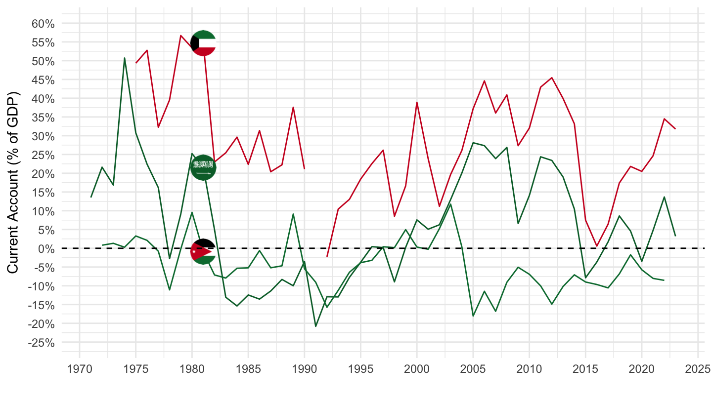
Canada, Israel, The Netherlands
Code
BN.CAB.XOKA.GD.ZS %>%
  filter(iso2c %in% c("CA", "IL", "NL")) %>%
  year_to_date %>%
  left_join(iso2c, by = "iso2c") %>%
  left_join(colors, by = c("Iso2c" = "country")) %>%
  mutate(value = value/100) %>%
  ggplot(.) +
  geom_line(aes(x = date, y = value, color = color)) +
  theme_minimal() + scale_color_identity() + add_3flags +
  scale_x_date(breaks = seq(1950, 2100, 5) %>% paste0("-01-01") %>% as.Date,
               labels = date_format("%Y")) +
  scale_y_continuous(breaks = 0.01*seq(-60, 60, 2),
                     labels = scales::percent_format(accuracy = 1)) +
  xlab("") + ylab("Current Account (% of GDP)") +
  geom_hline(yintercept = 0, linetype = "dashed",  color = "black")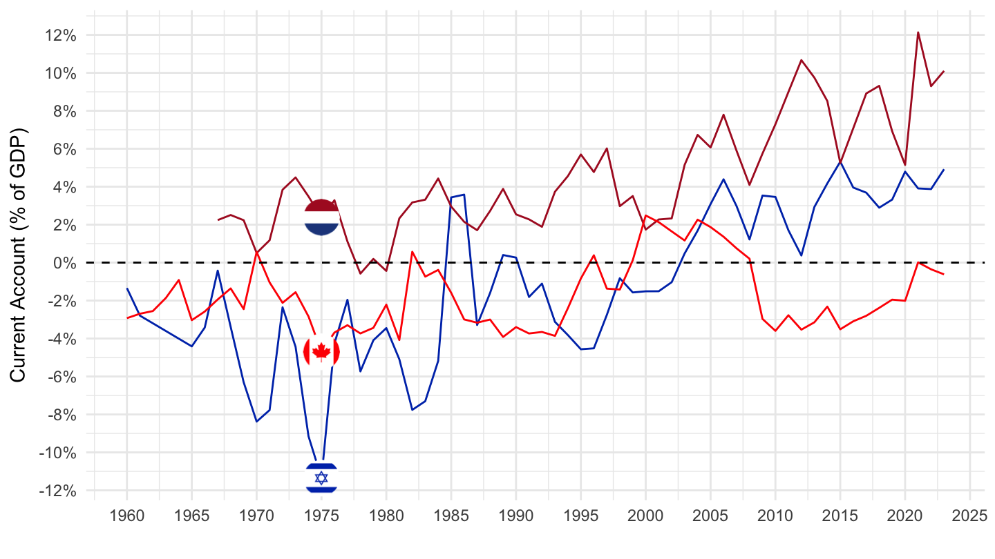
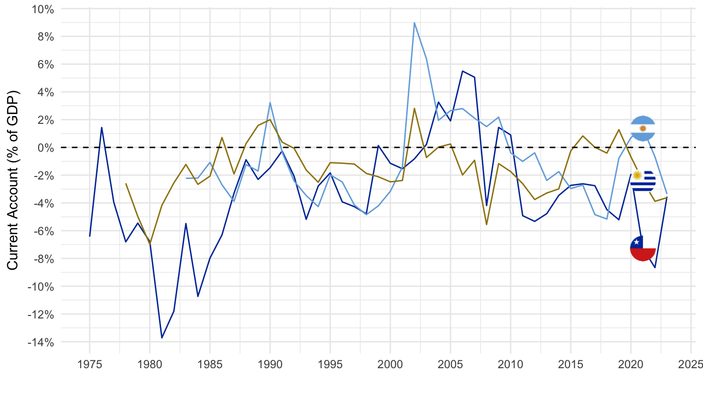
Argentina, Chile, Uruguay
Code
BN.CAB.XOKA.GD.ZS %>%
  filter(iso2c %in% c("AR", "CL", "UY")) %>%
  year_to_date %>%
  left_join(iso2c, by = "iso2c") %>%
  left_join(colors, by = c("Iso2c" = "country")) %>%
  mutate(value = value/100) %>%
  ggplot(.) +
  geom_line(aes(x = date, y = value, color = color)) +
  theme_minimal() + scale_color_identity() + add_3flags +
  scale_x_date(breaks = seq(1950, 2100, 5) %>% paste0("-01-01") %>% as.Date,
               labels = date_format("%Y")) +
  scale_y_continuous(breaks = 0.01*seq(-60, 60, 2),
                     labels = scales::percent_format(accuracy = 1)) +
  xlab("") + ylab("Current Account (% of GDP)") +
  geom_hline(yintercept = 0, linetype = "dashed",  color = "black")