OECD Data Live dataset

Data - OECD

Author

Info

source	dataset	Title	.html	.rData
oecd	DP_LIVE	OECD Data Live dataset	2025-11-17	2025-05-24

Data on macro

source	dataset	Title	.html	.rData
eurostat	nama_10_a10	Gross value added and income by A*10 industry breakdowns	2025-12-25	2025-12-25
eurostat	nama_10_a10_e	Employment by A*10 industry breakdowns	2025-12-25	2025-12-25
eurostat	nama_10_gdp	GDP and main components (output, expenditure and income)	2025-12-25	2025-12-25
eurostat	nama_10_lp_ulc	Labour productivity and unit labour costs	2025-12-25	2025-12-25
eurostat	namq_10_a10	Gross value added and income A*10 industry breakdowns	2025-12-25	2025-12-25
eurostat	namq_10_a10_e	Employment A*10 industry breakdowns	2025-05-24	2025-12-25
eurostat	namq_10_gdp	GDP and main components (output, expenditure and income)	2025-10-27	2025-12-25
eurostat	namq_10_lp_ulc	Labour productivity and unit labour costs	2025-12-25	2025-12-25
eurostat	namq_10_pc	Main GDP aggregates per capita	2025-12-25	2025-12-25
eurostat	nasa_10_nf_tr	Non-financial transactions	2025-12-25	2025-12-25
eurostat	nasq_10_nf_tr	Non-financial transactions	2025-12-25	2025-12-25
fred	gdp	Gross Domestic Product	2025-12-25	2025-12-25
oecd	QNA	Quarterly National Accounts	2024-06-06	2025-05-24
oecd	SNA_TABLE1	Gross domestic product (GDP)	2025-11-17	2025-05-24
oecd	SNA_TABLE14A	Non-financial accounts by sectors	2025-11-17	2024-06-30
oecd	SNA_TABLE2	Disposable income and net lending - net borrowing	2024-07-01	2024-04-11
oecd	SNA_TABLE6A	Value added and its components by activity, ISIC rev4	2024-07-01	2024-06-30
wdi	NE.RSB.GNFS.ZS	External balance on goods and services (% of GDP)	2025-12-24	2025-12-24
wdi	NY.GDP.MKTP.CD	GDP (current USD)	2025-12-24	2025-12-24
wdi	NY.GDP.MKTP.PP.CD	GDP, PPP (current international D)	2025-12-24	2025-12-24
wdi	NY.GDP.PCAP.CD	GDP per capita (current USD)	2025-12-24	2025-12-24
wdi	NY.GDP.PCAP.KD	GDP per capita (constant 2015 USD)	2025-12-24	2025-12-24
wdi	NY.GDP.PCAP.PP.CD	GDP per capita, PPP (current international D)	2025-12-24	2025-12-24
wdi	NY.GDP.PCAP.PP.KD	GDP per capita, PPP (constant 2011 international D)	2025-12-24	2025-12-24

LAST_COMPILE

LAST_COMPILE
2025-12-26

Last

obsTime	Nobs
2019-Q4	3645

INDICATOR

Code

DP_LIVE %>%
  left_join(DP_LIVE_var$INDICATOR, by = "INDICATOR") %>%
  group_by(INDICATOR, Indicator) %>%
  summarise(Nobs = n()) %>%
  arrange(-Nobs) %>%
  print_table_conditional()

SUBJECT

Code

DP_LIVE %>%
  left_join(DP_LIVE_var$SUBJECT, by = "SUBJECT") %>%
  group_by(SUBJECT, Subject) %>%
  summarise(Nobs = n()) %>%
  arrange(-Nobs) %>%
  print_table_conditional()

INDICATOR, SUBJECT

Code

DP_LIVE %>%
  left_join(DP_LIVE_var$INDICATOR, by = "INDICATOR") %>%
  left_join(DP_LIVE_var$SUBJECT, by = "SUBJECT") %>%
  group_by(INDICATOR, Indicator, SUBJECT, Subject) %>%
  summarise(Nobs = n()) %>%
  arrange(-Nobs) %>%
  print_table_conditional()

MEASURE

Code

DP_LIVE %>%
  left_join(DP_LIVE_var$MEASURE, by = "MEASURE") %>%
  group_by(MEASURE, Measure) %>%
  summarise(Nobs = n()) %>%
  arrange(-Nobs) %>%
  print_table_conditional()

LOCATION

Code

DP_LIVE %>%
  left_join(DP_LIVE_var$LOCATION, by = "LOCATION") %>%
  group_by(LOCATION, Location) %>%
  summarise(Nobs = n()) %>%
  arrange(-Nobs) %>%
  mutate(Flag = gsub(" ", "-", str_to_lower(gsub(" ", "-", Location))),
         Flag = paste0('<img src="../../icon/flag/vsmall/', Flag, '.png" alt="Flag">')) %>%
  select(Flag, everything()) %>%
  {if (is_html_output()) datatable(., filter = 'top', rownames = F, escape = F) else .}

FREQUENCY

Code

DP_LIVE %>%
  left_join(DP_LIVE_var$FREQUENCY, by = "FREQUENCY") %>%
  group_by(FREQUENCY, Frequency) %>%
  summarise(Nobs = n()) %>%
  arrange(-Nobs) %>%
  print_table_conditional()

FREQUENCY	Frequency	Nobs
A	Annual	1230866
M	Monthly	694441
Q	Quarterly	476659

INDICATOR, SUBJECT, FREQUENCY

Code

DP_LIVE %>%
  left_join(DP_LIVE_var$INDICATOR, by = "INDICATOR") %>%
  left_join(DP_LIVE_var$SUBJECT, by = "SUBJECT") %>%
  group_by(INDICATOR, Indicator, SUBJECT, Subject, FREQUENCY) %>%
  summarise(Nobs = n()) %>%
  arrange(-Nobs) %>%
  print_table_conditional()

obsTime

Code

DP_LIVE %>%
  group_by(obsTime) %>%
  summarise(Nobs = n()) %>%
  arrange(desc(obsTime)) %>%
  print_table_conditional()

Saving Rate - SAVING

See: https://data.oecd.org/natincome/saving-rate.htm

Saving is equal to the difference between disposable income (including an adjustment for the change in employment-related pension entitlements) and final consumption expenditure. It reflects the part of disposable income that, together with the incurrence of liabilities, is available to acquire financial and non-financial assets. The saving rate presented here corresponds to net saving, which is saving net of depreciation, as percentage of gross domestic product (GDP). All OECD countries compile their data according to the 2008 System of National Accounts (SNA).

United States, France

Code

DP_LIVE %>%
  filter(INDICATOR == "SAVING",
         LOCATION %in% c("FRA", "USA"),
         SUBJECT == "TOT",
         MEASURE == "PC_GDP") %>%
  left_join(DP_LIVE_var$LOCATION, by = "LOCATION") %>%
  year_to_date() %>%
  left_join(colors, by = c("Location" = "country")) %>%
  mutate(obsValue = obsValue/100) %>%
  ggplot(.) + geom_line(aes(x = date, y = obsValue, color = color)) +
  theme_minimal() + xlab("") + ylab("Saving Rate (% of GDP)") +
  add_2flags + scale_color_identity() +
  scale_y_continuous(breaks = 0.01*seq(-100, 260, 2),
                     labels = percent_format(accuracy = 1, p = "")) +
  scale_x_date(breaks = as.Date(paste0(seq(1700, 2100, 5), "-01-01")),
               labels = date_format("%Y"))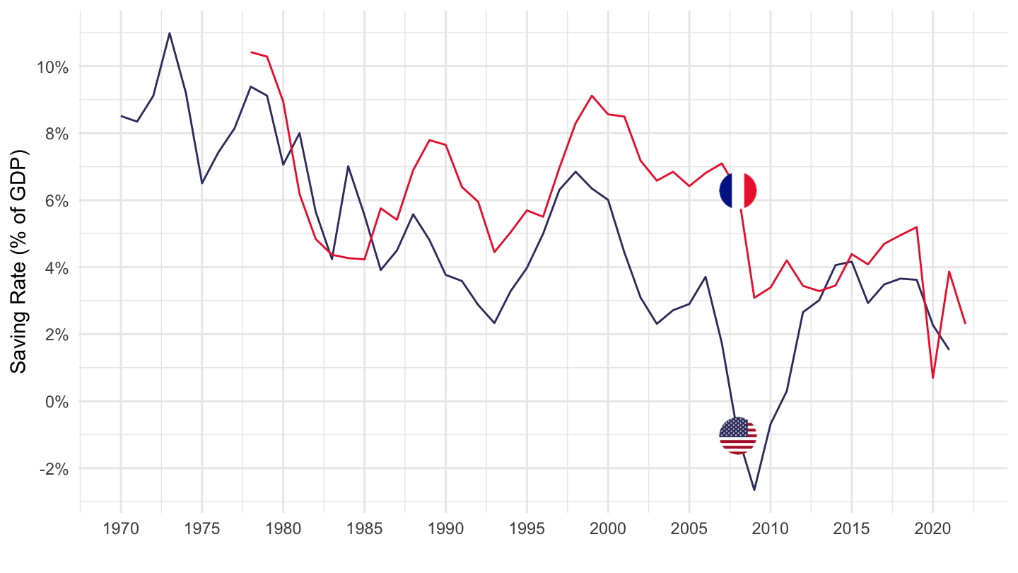

United States, France, Germany, Italy

Code

DP_LIVE %>%
  filter(INDICATOR == "SAVING",
         LOCATION %in% c("FRA", "USA", "DEU", "ITA"),
         SUBJECT == "TOT",
         MEASURE == "PC_GDP") %>%
  left_join(DP_LIVE_var$LOCATION, by = "LOCATION") %>%
  year_to_date() %>%
  left_join(colors, by = c("Location" = "country")) %>%
  mutate(obsValue = obsValue/100) %>%
  ggplot(.) + geom_line(aes(x = date, y = obsValue, color = color)) +
  theme_minimal() + xlab("") + ylab("Saving Rate (% of GDP)") +
  add_4flags + scale_color_identity() +
  scale_y_continuous(breaks = 0.01*seq(-100, 260, 2),
                     labels = percent_format(accuracy = 1, p = "")) +
  scale_x_date(breaks = as.Date(paste0(seq(1700, 2100, 5), "-01-01")),
               labels = date_format("%Y"))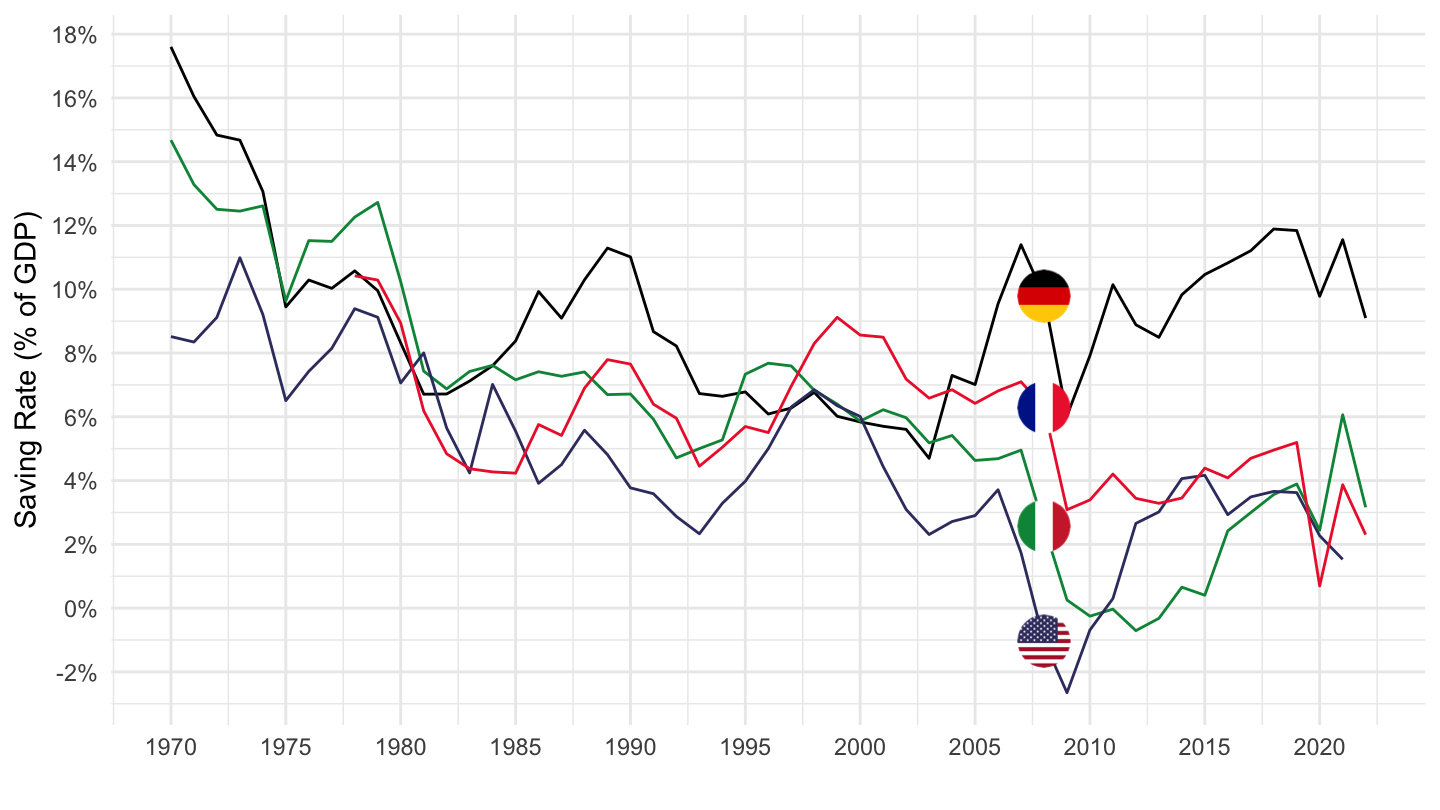

Money

Narrow Money - M1

Table

Code

DP_LIVE %>%
  filter(INDICATOR == "M1",
         FREQUENCY == "M") %>%
  left_join(DP_LIVE_var$LOCATION, by = "LOCATION") %>%
  select_if(~ n_distinct(.) > 1) %>%
  group_by(LOCATION, Location) %>%
  summarise(Nobs = n(),
            obsValue = last(obsValue)) %>%
  arrange(-obsValue) %>%
  mutate(Flag = gsub(" ", "-", str_to_lower(gsub(" ", "-", Location))),
         Flag = paste0('<img src="../../icon/flag/vsmall/', Flag, '.png" alt="Flag">')) %>%
  select(Flag, everything()) %>%
  {if (is_html_output()) datatable(., filter = 'top', rownames = F, escape = F) else .}

Japan, United Kingdom, USA

Code

DP_LIVE %>%
  filter(LOCATION %in% c("JPN", "GBR", "USA"),
         INDICATOR == "M1",
         FREQUENCY == "M") %>%
  month_to_date %>%
  left_join(DP_LIVE_var$LOCATION, by = "LOCATION") %>%
  group_by(LOCATION) %>%
  left_join(colors, by = c("Location" = "country")) %>%
  ggplot(.) + geom_line(aes(x = date, y = obsValue, color = color)) + 
  scale_color_identity() + add_3flags +
  theme_minimal() + xlab("") + ylab("Narrow Money - M1") +
  scale_x_date(breaks = seq(1940, 2030, 5) %>% paste0("-01-01") %>% as.Date,
               labels = date_format("%Y")) +
  scale_y_log10(breaks = c(1, 2, 3, 5, 10, 20, 50, 80, 100, 200, 300, 500, 800))

Euro area, U.S.

Code

DP_LIVE %>%
  filter(LOCATION %in% c("EA19", "USA", "JPN"),
         INDICATOR == "M1",
         FREQUENCY == "M") %>%
  month_to_date %>%
  left_join(DP_LIVE_var$LOCATION, by = "LOCATION") %>%
  group_by(LOCATION) %>%
  left_join(colors, by = c("Location" = "country")) %>%
  mutate(Location = ifelse(LOCATION == "EA19", "Europe", Location)) %>%
  ggplot(.) + geom_line(aes(x = date, y = obsValue, color = color)) + 
  scale_color_identity() + add_3flags +
  theme_minimal() + xlab("") + ylab("Narrow Money - M1") +
  scale_x_date(breaks = seq(1940, 2030, 5) %>% paste0("-01-01") %>% as.Date,
               labels = date_format("%Y")) +
  scale_y_log10(breaks = c(1, 2, 3, 5, 10, 20, 50, 80, 100, 200, 300, 500, 800))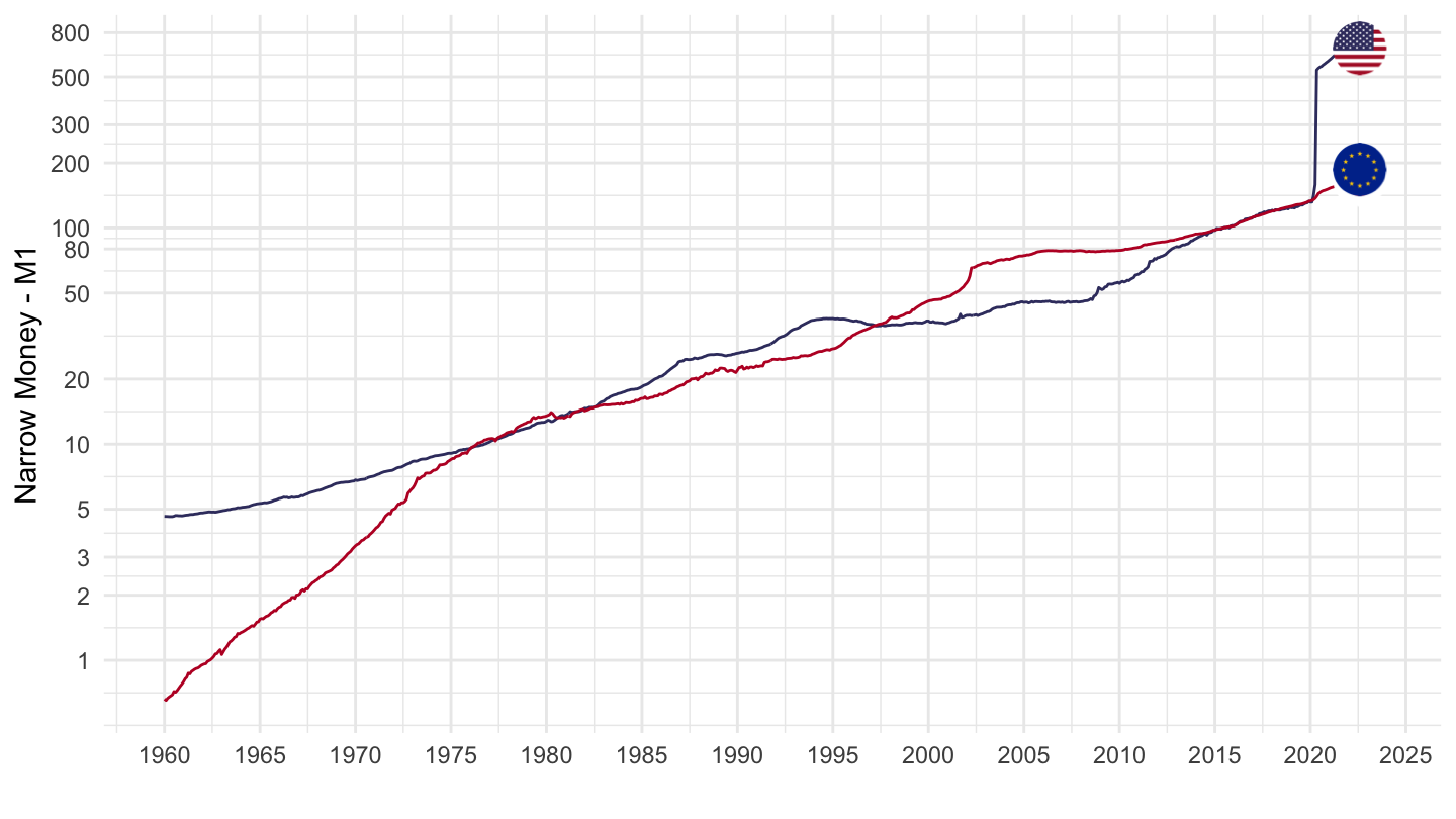

Broad Money - M3

Table

Code

DP_LIVE %>%
  filter(INDICATOR == "M3",
         FREQUENCY == "M") %>%
  left_join(DP_LIVE_var$LOCATION, by = "LOCATION") %>%
  select_if(~ n_distinct(.) > 1) %>%
  group_by(LOCATION, Location) %>%
  summarise(Nobs = n(),
            obsValue = last(obsValue)) %>%
  arrange(-obsValue) %>%
  mutate(Flag = gsub(" ", "-", str_to_lower(gsub(" ", "-", Location))),
         Flag = paste0('<img src="../../icon/flag/vsmall/', Flag, '.png" alt="Flag">')) %>%
  select(Flag, everything()) %>%
  {if (is_html_output()) datatable(., filter = 'top', rownames = F, escape = F) else .}

Japan, United Kingdom, USA

Code

DP_LIVE %>%
  filter(LOCATION %in% c("JPN", "GBR", "USA"),
         INDICATOR == "M3",
         FREQUENCY == "M") %>%
  month_to_date %>%
  left_join(DP_LIVE_var$LOCATION, by = "LOCATION") %>%
  group_by(LOCATION) %>%
  left_join(colors, by = c("Location" = "country")) %>%
  ggplot(.) + geom_line(aes(x = date, y = obsValue, color = color)) + 
  scale_color_identity() + add_3flags +
  theme_minimal() + xlab("") + ylab("Broad Money - M3") +
  scale_x_date(breaks = seq(1940, 2030, 5) %>% paste0("-01-01") %>% as.Date,
               labels = date_format("%Y")) +
  scale_y_log10(breaks = c(1, 2, 3, 5, 10, 20, 50, 80, 100, 200, 300, 500, 800))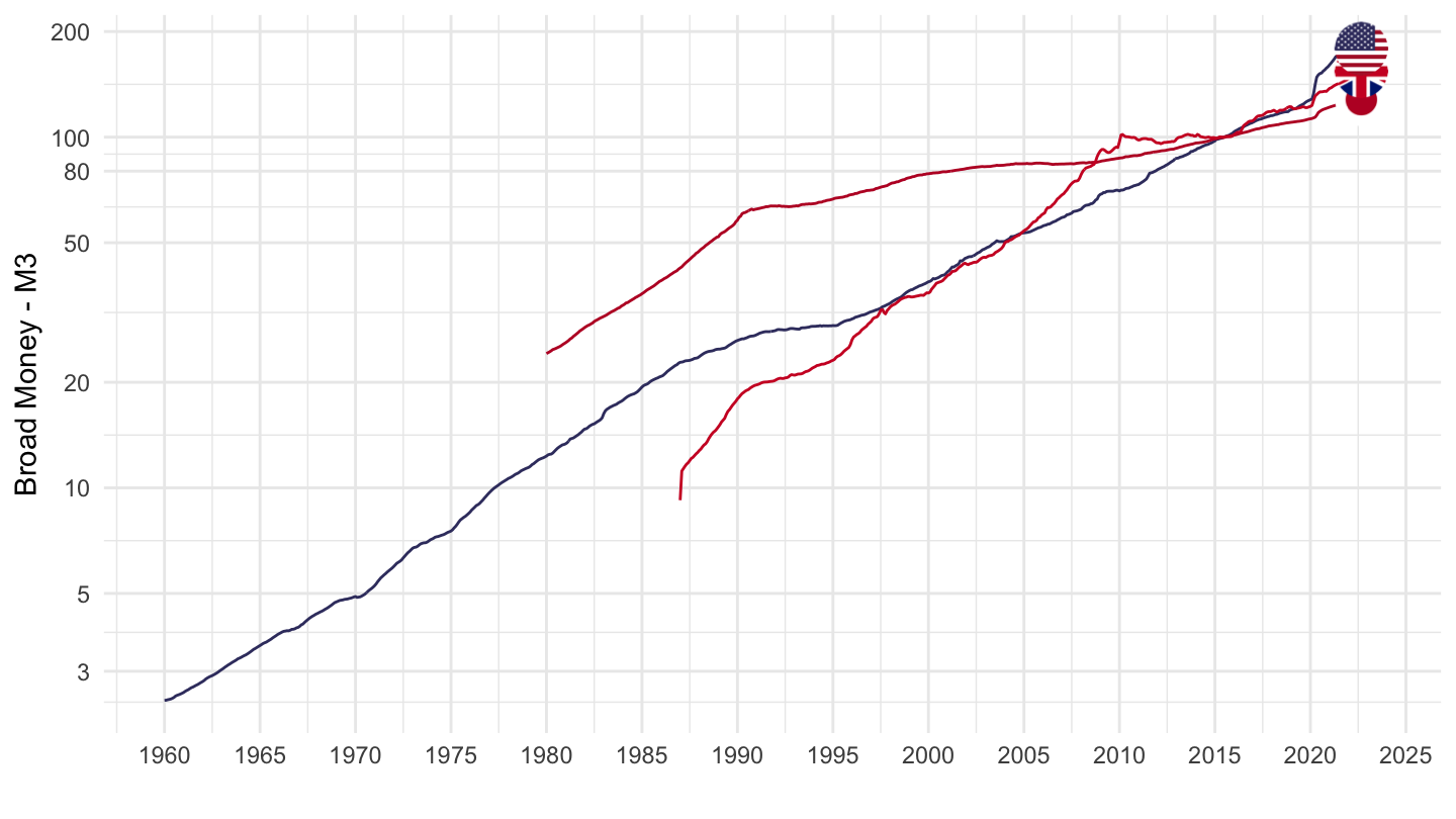

Euro area, U.S.

Code

DP_LIVE %>%
  filter(LOCATION %in% c("EA19", "USA", "JPN"),
         INDICATOR == "M3",
         FREQUENCY == "M") %>%
  month_to_date %>%
  left_join(DP_LIVE_var$LOCATION, by = "LOCATION") %>%
  group_by(LOCATION) %>%
  left_join(colors, by = c("Location" = "country")) %>%
  mutate(Location = ifelse(LOCATION == "EA19", "Europe", Location)) %>%
  ggplot(.) + geom_line(aes(x = date, y = obsValue, color = color)) + 
  scale_color_identity() + add_3flags +
  theme_minimal() + xlab("") + ylab("Broad Money - M3") +
  scale_x_date(breaks = seq(1940, 2030, 5) %>% paste0("-01-01") %>% as.Date,
               labels = date_format("%Y")) +
  scale_y_log10(breaks = c(1, 2, 3, 5, 10, 20, 50, 80, 100, 200, 300, 500, 800))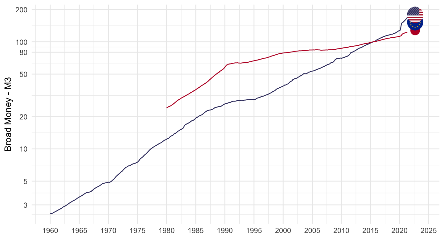

Gross domestic spending on R&D - GDEXPRD

Table

Code

DP_LIVE %>%
  filter(INDICATOR == "GDEXPRD",
         SUBJECT == "TOT",
         MEASURE == "PC_GDP") %>%
  left_join(DP_LIVE_var$LOCATION, by = "LOCATION") %>%
  group_by(LOCATION, Location) %>%
  arrange(obsTime) %>%
  summarise(date_min = min(obsTime),
            date_max = max(obsTime),
            obsValue = last(obsValue)) %>%
  arrange(-obsValue) %>%
  mutate(Flag = gsub(" ", "-", str_to_lower(gsub(" ", "-", Location))),
         Flag = paste0('<img src="../../icon/flag/vsmall/', Flag, '.png" alt="Flag">')) %>%
  select(Flag, everything()) %>%
  {if (is_html_output()) datatable(., filter = 'top', rownames = F, escape = F) else .}

Korea, Israel, Sweden, Japan, Taiwan

Code

DP_LIVE %>%
  filter(INDICATOR == "GDEXPRD",
         LOCATION %in% c("KOR", "ISR", "SWE", "JPN", "TWN"),
         SUBJECT == "TOT",
         MEASURE == "PC_GDP") %>%
  left_join(DP_LIVE_var$LOCATION, by = "LOCATION") %>%
  year_to_date() %>%
  mutate(Location = ifelse(LOCATION == "TWN", "Taiwan", Location)) %>%
  left_join(colors, by = c("Location" = "country")) %>%
  mutate(Location = ifelse(LOCATION == "TWN", "Taiwan", Location)) %>%
  mutate(obsValue = obsValue/100) %>%
  ggplot(.) + geom_line(aes(x = date, y = obsValue, color = color)) +
  theme_minimal() + xlab("") + ylab("Gross domestic spending on R&D") +
  add_5flags + scale_color_identity() +
  scale_y_continuous(breaks = 0.01*seq(0, 260, .2),
                     labels = percent_format(accuracy = .1, p = "")) +
  scale_x_date(breaks = as.Date(paste0(seq(1700, 2100, 5), "-01-01")),
               labels = date_format("%Y"))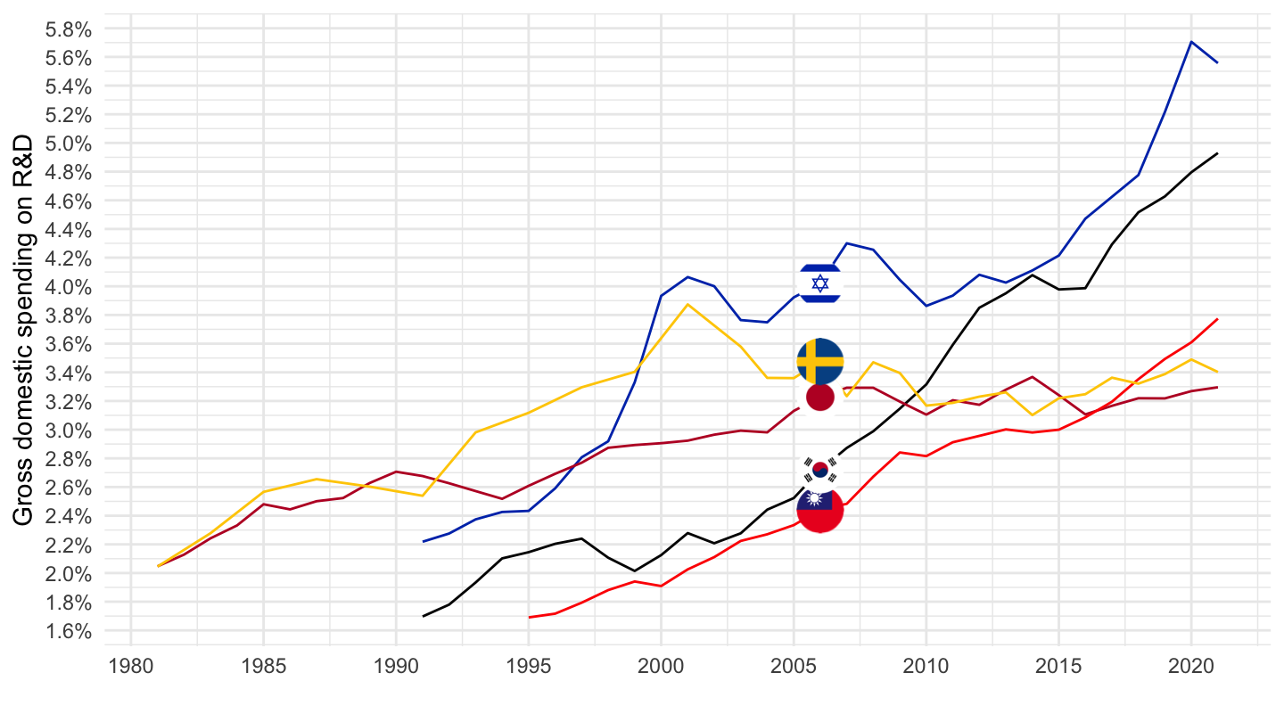

United States, France, Germany, Italy, Japan

Code

DP_LIVE %>%
  filter(INDICATOR == "GDEXPRD",
         LOCATION %in% c("USA", "FRA", "DEU", "ITA", "JPN"),
         SUBJECT == "TOT",
         MEASURE == "PC_GDP") %>%
  left_join(DP_LIVE_var$LOCATION, by = "LOCATION") %>%
  year_to_date() %>%
  left_join(colors, by = c("Location" = "country")) %>%
  mutate(obsValue = obsValue/100) %>%
  ggplot(.) + geom_line(aes(x = date, y = obsValue, color = color)) +
  theme_minimal() + xlab("") + ylab("Gross domestic spending on R&D") +
  add_5flags + scale_color_identity() +
  scale_y_continuous(breaks = 0.01*seq(0, 260, .2),
                     labels = percent_format(accuracy = .1, p = "")) +
  scale_x_date(breaks = as.Date(paste0(seq(1700, 2100, 5), "-01-01")),
               labels = date_format("%Y"))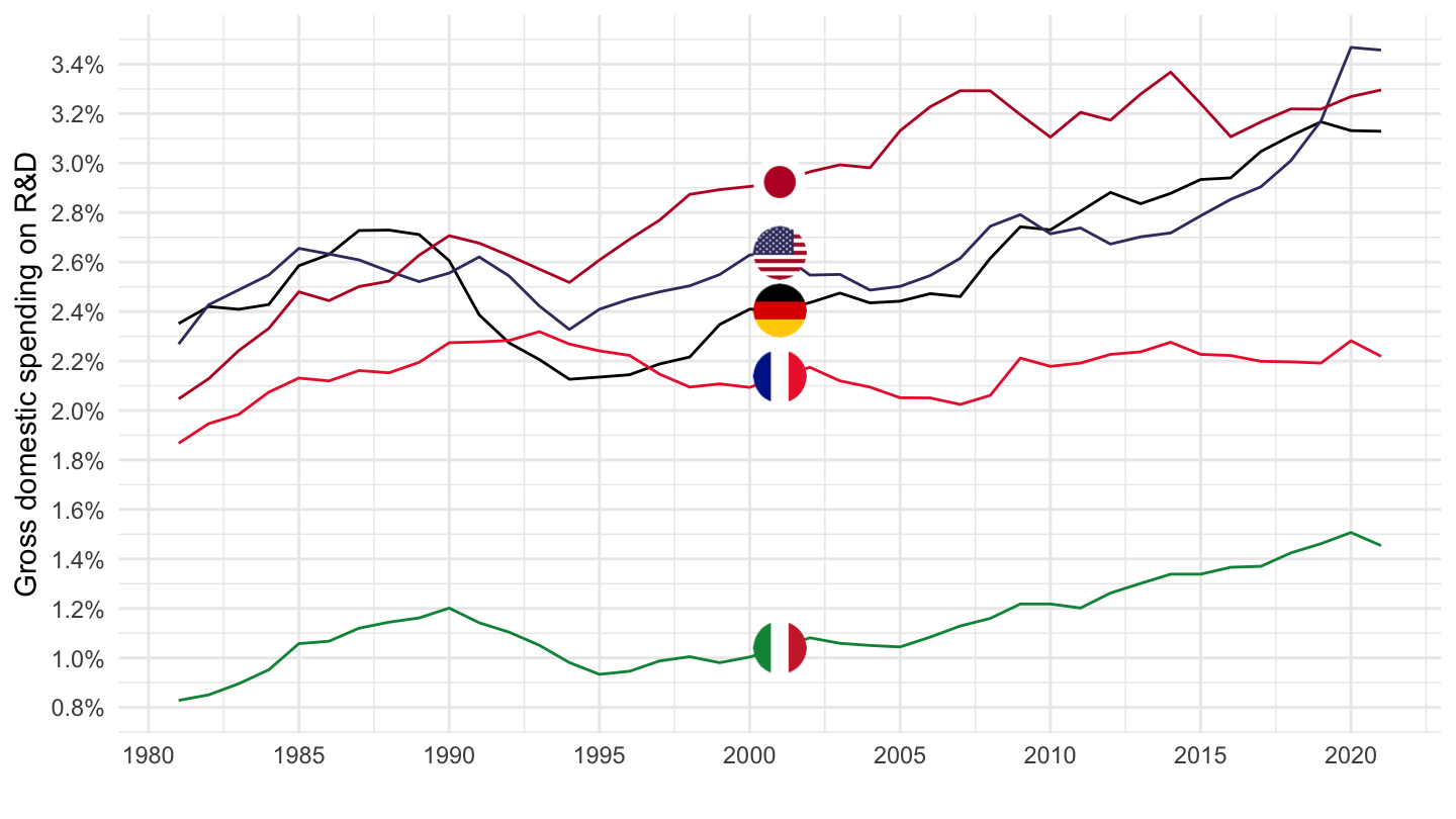

Spain, Portugal

Code

DP_LIVE %>%
  filter(INDICATOR == "GDEXPRD",
         LOCATION %in% c("ESP", "PRT"),
         SUBJECT == "TOT",
         MEASURE == "PC_GDP") %>%
  left_join(DP_LIVE_var$LOCATION, by = "LOCATION") %>%
  year_to_date() %>%
  left_join(colors, by = c("Location" = "country")) %>%
  mutate(obsValue = obsValue/100) %>%
  ggplot(.) + geom_line(aes(x = date, y = obsValue, color = color)) +
  theme_minimal() + xlab("") + ylab("Gross domestic spending on R&D") +
  add_2flags + scale_color_identity() +
  scale_y_continuous(breaks = 0.01*seq(0, 260, .2),
                     labels = percent_format(accuracy = .1, p = "")) +
  scale_x_date(breaks = as.Date(paste0(seq(1700, 2100, 5), "-01-01")),
               labels = date_format("%Y"))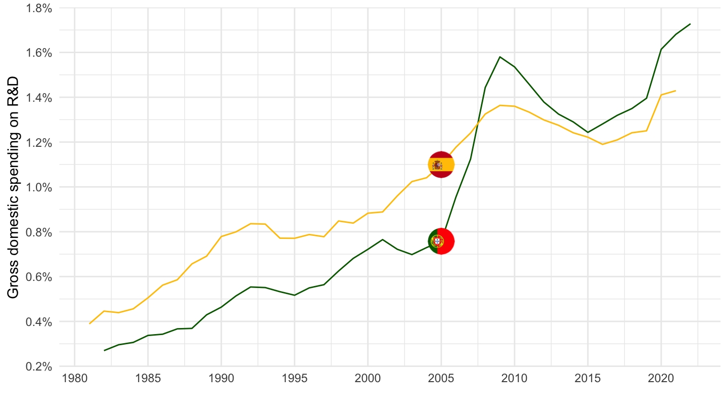

Social Spending - SOCEXP, PENSIONEXP

Table

Code

DP_LIVE %>%
  filter(INDICATOR %in% c("SOCEXP", "PENSIONEXP"),
         MEASURE == "PC_GDP",
         obsTime == "2019") %>%
  left_join(DP_LIVE_var$LOCATION, by = "LOCATION") %>%
  filter(!is.na(obsValue)) %>%
  group_by(LOCATION, Location) %>%
  arrange(obsTime) %>%
  summarise(date_min = min(obsTime),
            date_max = max(obsTime),
            obsValue = last(obsValue)) %>%
  mutate(obsValue = obsValue/10^6/0.14) %>%
  arrange(-obsValue) %>%
  mutate(Flag = gsub(" ", "-", str_to_lower(gsub(" ", "-", Location))),
         Flag = paste0('<img src="../../icon/flag/vsmall/', Flag, '.png" alt="Flag">')) %>%
  select(Flag, everything()) %>%
  {if (is_html_output()) datatable(., filter = 'top', rownames = F, escape = F) else .}

OILPROD - Crude oil production

Info

Crude oil production in DP_LIVE is expressed as KTOE - thousands of ton of oil equivalent. (toe)

95 Millions of barrels / day = 34.7 Bn of barrels / year
1 barrel of oil equivalent (boe) = 0.14 ton of oil equivalent (toe).
1 ton of oil equivalent = 1/0.14 = 7.14 barrels of oil equivalent.

Table

Code

DP_LIVE %>%
  filter(INDICATOR == "OILPROD") %>%
  left_join(DP_LIVE_var$LOCATION, by = "LOCATION") %>%
  select_if(~ n_distinct(.) > 1) %>%
  filter(!is.na(obsValue)) %>%
  group_by(LOCATION, Location) %>%
  arrange(obsTime) %>%
  summarise(date_min = min(obsTime),
            date_max = max(obsTime),
            obsValue = last(obsValue)) %>%
  mutate(obsValue = obsValue/10^6/0.14) %>%
  arrange(-obsValue) %>%
  mutate(Flag = gsub(" ", "-", str_to_lower(gsub(" ", "-", Location))),
         Flag = paste0('<img src="../../icon/flag/vsmall/', Flag, '.png" alt="Flag">')) %>%
  select(Flag, everything()) %>%
  {if (is_html_output()) datatable(., filter = 'top', rownames = F, escape = F) else .}

Table - World

Code

OILPRODWLD <- DP_LIVE %>%
  filter(INDICATOR == "OILPROD",
         LOCATION == "WLD") %>%
  select_if(~n_distinct(.) > 1) %>%
  filter(!is.na(obsValue)) %>%
  year_to_date %>%
  transmute(date, variable = "OILPRODWLD", value = obsValue)

save(OILPRODWLD, file = "DP_LIVE_OILPRODWLD.RData")

World, Saudi Arabia, Russia

Code

DP_LIVE %>%
  filter(INDICATOR == "OILPROD",
         LOCATION %in% c("WLD", "RUS", "SAU")) %>%
  left_join(DP_LIVE_var$LOCATION, by = "LOCATION") %>%
  left_join(DP_LIVE_var$INDICATOR, by = "INDICATOR") %>%
  filter(!is.na(obsValue)) %>%
  year_to_date() %>%
  left_join(colors, by = c("Location" = "country")) %>%
  mutate(obsValue = obsValue/10^6/0.14) %>%
  # 0.14 = 
  ggplot(.) + geom_line(aes(x = date, y = obsValue, color = color)) +
  theme_minimal() + xlab("") + ylab("Billions of Barrels of Oil") +
  add_3flags + scale_color_identity() +
  scale_y_log10(breaks = c(1, 2, 3, 4, 5, 8, 10, 15, 20, 30),
                labels = dollar_format(a = 1, pre = "", su = " Bn")) +
  scale_x_date(breaks = as.Date(paste0(seq(1700, 2100, 5), "-01-01")),
               labels = date_format("%Y"))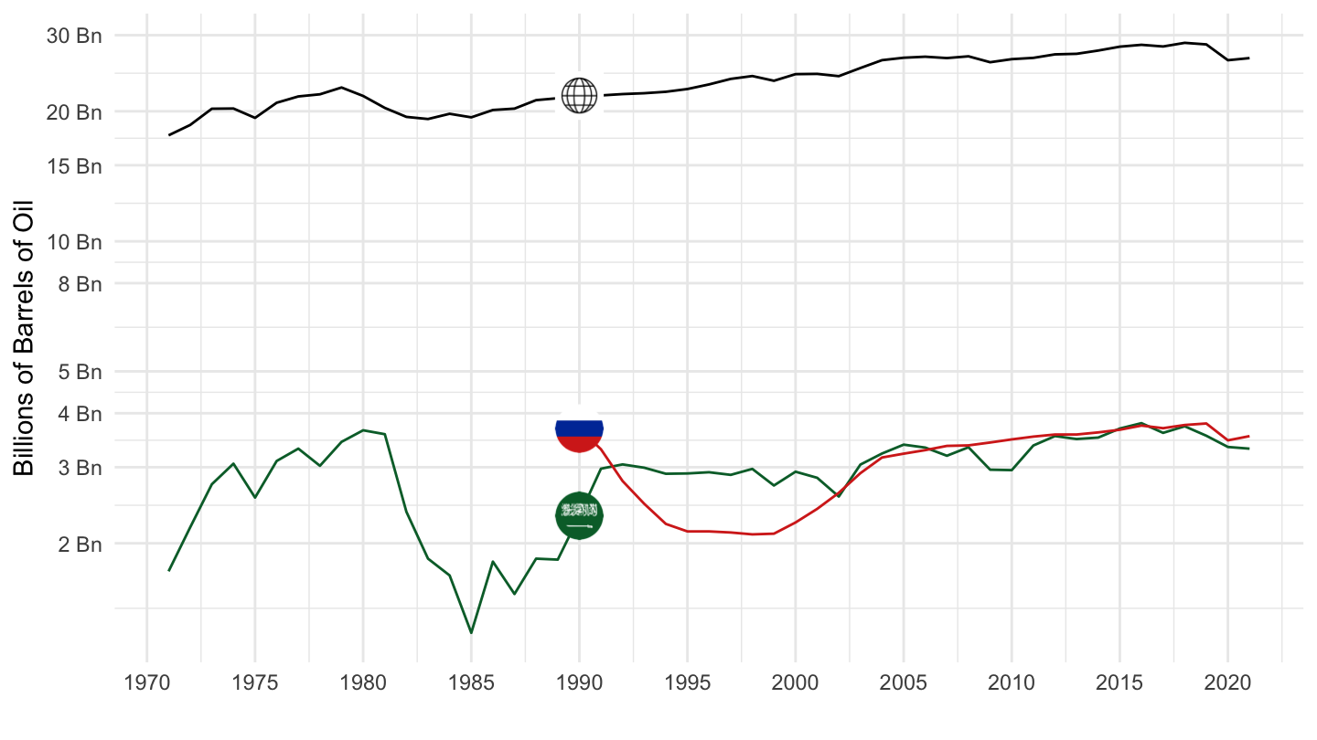

USA, Iraq, Iran

Code

DP_LIVE %>%
  filter(INDICATOR == "OILPROD",
         LOCATION %in% c("USA", "IRQ", "IRN")) %>%
  left_join(DP_LIVE_var$LOCATION, by = "LOCATION") %>%
  left_join(DP_LIVE_var$INDICATOR, by = "INDICATOR") %>%
  filter(!is.na(obsValue)) %>%
  year_to_date() %>%
  left_join(colors, by = c("Location" = "country")) %>%
  mutate(obsValue = obsValue/10^6/0.14) %>%
  # 0.14 = 
  ggplot(.) + geom_line(aes(x = date, y = obsValue, color = color)) +
  theme_minimal() + xlab("") + ylab("Billions of Barrels of Oil") +
  add_3flags + scale_color_identity() +
  scale_y_log10(breaks = c(0.1, 0.2 ,0.5, 0.8, 1, 2, 3, 4, 5, 8, 10, 15, 20, 30),
                labels = dollar_format(a = .1, pre = "", su = " Bn")) +
  scale_x_date(breaks = as.Date(paste0(seq(1700, 2100, 5), "-01-01")),
               labels = date_format("%Y"))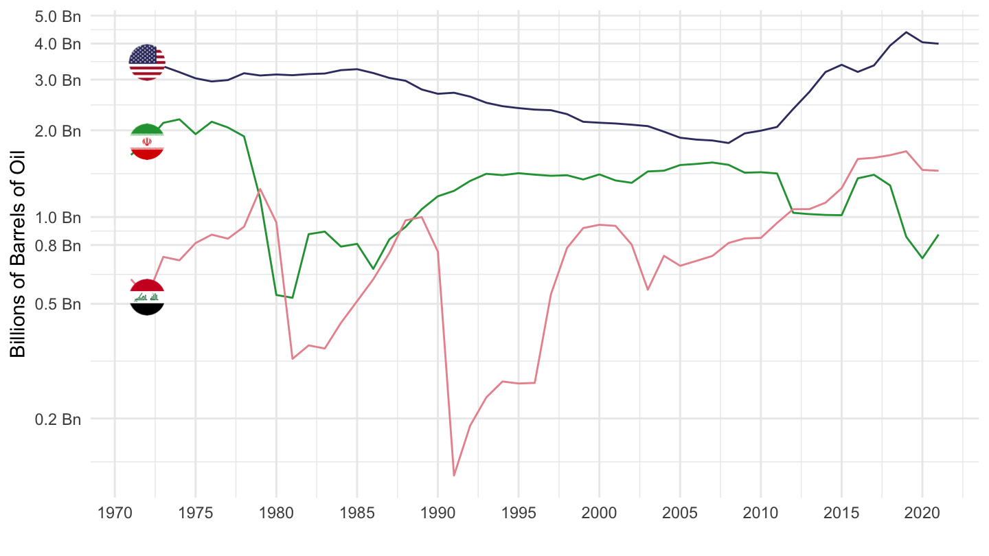

GGEXP - General government spending

Table

Code

DP_LIVE %>%
  filter(INDICATOR == "GGEXP",
         SUBJECT == "TOT",
         MEASURE == "PC_GDP") %>%
  left_join(DP_LIVE_var$LOCATION, by = "LOCATION") %>%
  group_by(LOCATION, Location) %>%
  arrange(obsTime) %>%
  summarise(date_min = min(obsTime),
            date_max = max(obsTime),
            obsValue = last(obsValue)) %>%
  arrange(-obsValue) %>%
  mutate(Flag = gsub(" ", "-", str_to_lower(gsub(" ", "-", Location))),
         Flag = paste0('<img src="../../icon/flag/vsmall/', Flag, '.png" alt="Flag">')) %>%
  select(Flag, everything()) %>%
  {if (is_html_output()) datatable(., filter = 'top', rownames = F, escape = F) else .}

United States, Europe

Code

DP_LIVE %>%
  filter(INDICATOR == "GGEXP",
         LOCATION %in% c("FRA", "USA"),
         SUBJECT == "TOT",
         MEASURE == "PC_GDP") %>%
  left_join(DP_LIVE_var$LOCATION, by = "LOCATION") %>%
  year_to_date() %>%
  left_join(colors, by = c("Location" = "country")) %>%
  mutate(obsValue = obsValue/100) %>%
  ggplot(.) + geom_line(aes(x = date, y = obsValue, color = color)) +
  theme_minimal() + xlab("") + ylab("General government spending") +
  add_2flags + scale_color_identity() +
  scale_y_continuous(breaks = 0.01*seq(0, 260, 2),
                     labels = percent_format(accuracy = 1, p = "")) +
  scale_x_date(breaks = as.Date(paste0(seq(1700, 2100, 5), "-01-01")),
               labels = date_format("%Y"))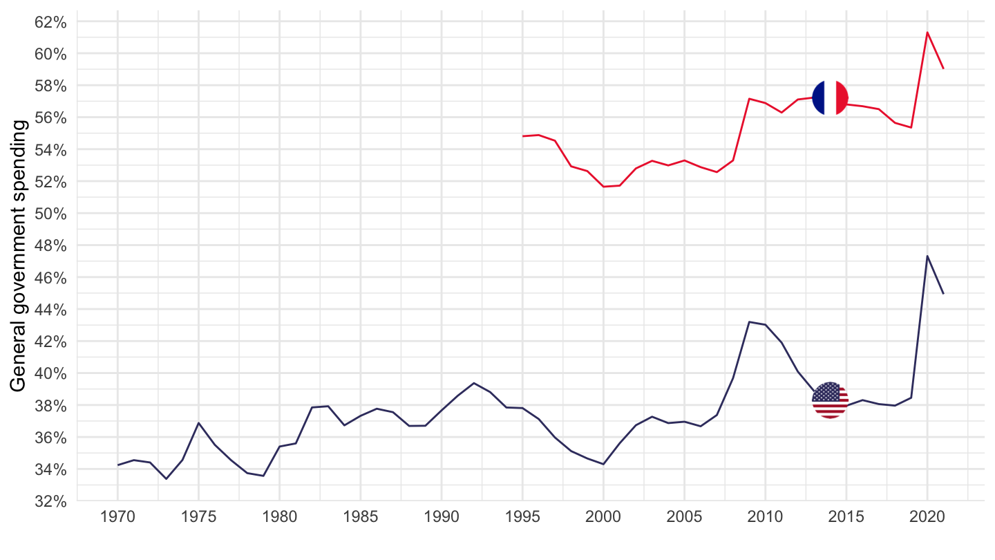

Spain, Italy, France, Germany, Portugal

Code

DP_LIVE %>%
  filter(INDICATOR == "GGEXP",
         LOCATION %in% c("ESP", "ITA", "FRA", "DEU", "PRT", "USA"),
         SUBJECT == "TOT",
         MEASURE == "PC_GDP") %>%
  left_join(DP_LIVE_var$LOCATION, by = "LOCATION") %>%
  year_to_date() %>%
  filter(date >= as.Date("1995-01-01")) %>%
  left_join(colors, by = c("Location" = "country")) %>%
  mutate(obsValue = obsValue/100) %>%
  ggplot(.) + geom_line(aes(x = date, y = obsValue, color = color)) +
  theme_minimal() + xlab("") + ylab("General government spending (% of GDP)") +
  add_6flags + scale_color_identity() +
  scale_y_continuous(breaks = 0.01*seq(0, 260, 2),
                     labels = percent_format(accuracy = 1, p = "")) +
  scale_x_date(breaks = as.Date(paste0(seq(1700, 2100, 5), "-01-01")),
               labels = date_format("%Y"))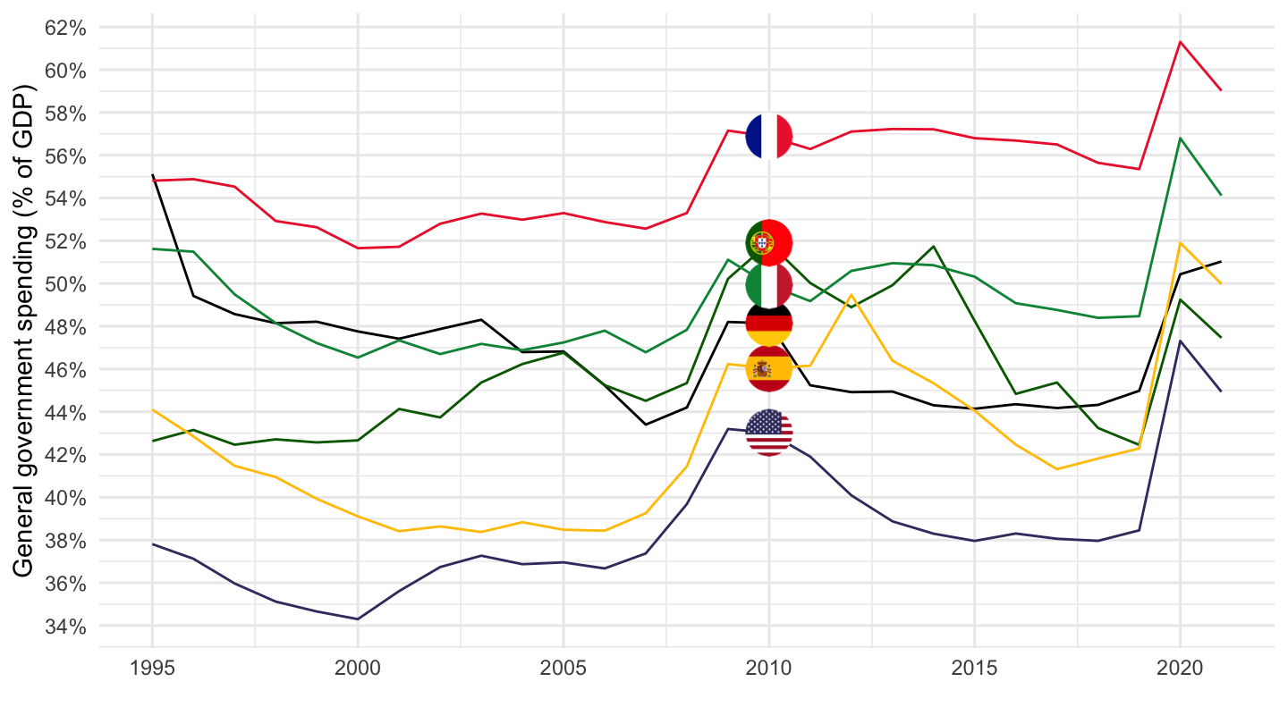

France, Finland, Belgium, Norway, Denmark

Code

DP_LIVE %>%
  filter(INDICATOR == "GGEXP",
         LOCATION %in% c("FRA", "FIN", "BEL", "NOR", "DNK"),
         SUBJECT == "TOT",
         MEASURE == "PC_GDP") %>%
  left_join(DP_LIVE_var$LOCATION, by = "LOCATION") %>%
  year_to_date() %>%
  left_join(colors, by = c("Location" = "country")) %>%
  mutate(obsValue = obsValue/100) %>%
  ggplot(.) + geom_line(aes(x = date, y = obsValue, color = color)) +
  theme_minimal() + xlab("") + ylab("General government spending") +
  add_5flags + scale_color_identity() +
  scale_y_continuous(breaks = 0.01*seq(0, 260, 2),
                     labels = percent_format(accuracy = 1, p = "")) +
  scale_x_date(breaks = as.Date(paste0(seq(1700, 2100, 5), "-01-01")),
               labels = date_format("%Y"))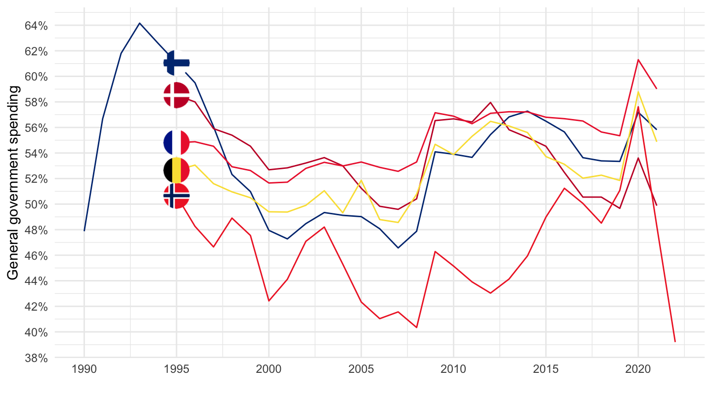

Sweden, Italy, Austria, Luxembourg, Greece

Code

DP_LIVE %>%
  filter(INDICATOR == "GGEXP",
         LOCATION %in% c("SWE", "ITA", "AUT", "LUX", "GRC"),
         SUBJECT == "TOT",
         MEASURE == "PC_GDP") %>%
  left_join(DP_LIVE_var$LOCATION, by = "LOCATION") %>%
  year_to_date() %>%
  left_join(colors, by = c("Location" = "country")) %>%
  mutate(obsValue = obsValue/100) %>%
  ggplot(.) + geom_line(aes(x = date, y = obsValue, color = color)) +
  theme_minimal() + xlab("") + ylab("General government spending") +
  add_5flags + scale_color_identity() +
  scale_y_continuous(breaks = 0.01*seq(0, 260, 2),
                     labels = percent_format(accuracy = 1, p = "")) +
  scale_x_date(breaks = as.Date(paste0(seq(1700, 2100, 5), "-01-01")),
               labels = date_format("%Y"))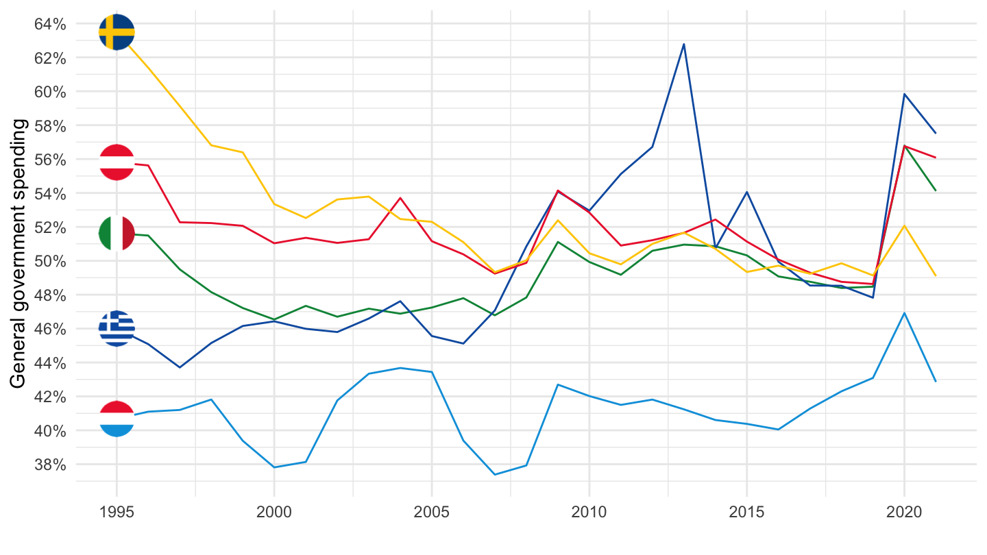

Hungary, Germany, Australia, Iceland, Slovenia

Code

DP_LIVE %>%
  filter(INDICATOR == "GGEXP",
         LOCATION %in% c("HUN", "DEU", "AUS", "ISL", "SVN"),
         SUBJECT == "TOT",
         MEASURE == "PC_GDP") %>%
  left_join(DP_LIVE_var$LOCATION, by = "LOCATION") %>%
  year_to_date() %>%
  left_join(colors, by = c("Location" = "country")) %>%
  mutate(obsValue = obsValue/100) %>%
  ggplot(.) + geom_line(aes(x = date, y = obsValue, color = color)) +
  theme_minimal() + xlab("") + ylab("General government spending") +
  add_5flags + scale_color_identity() +
  scale_y_continuous(breaks = 0.01*seq(0, 260, 2),
                     labels = percent_format(accuracy = 1, p = "")) +
  scale_x_date(breaks = as.Date(paste0(seq(1700, 2100, 5), "-01-01")),
               labels = date_format("%Y"))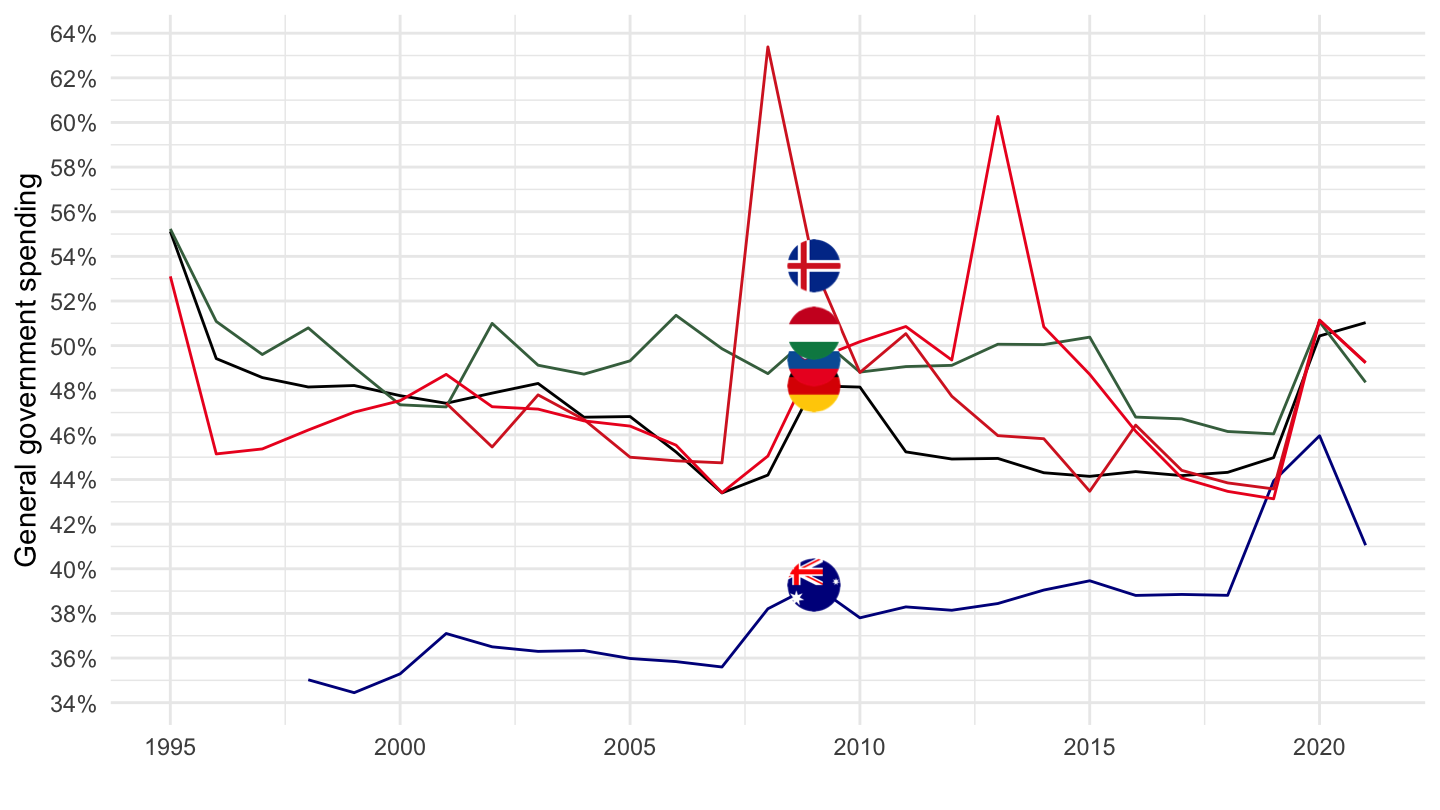

Slovak Republic, Portugal, Spain, Netherlands, Poland

Code

DP_LIVE %>%
  filter(INDICATOR == "GGEXP",
         LOCATION %in% c("SVK", "PRT", "ESP", "NLD", "POL"),
         SUBJECT == "TOT",
         MEASURE == "PC_GDP") %>%
  left_join(DP_LIVE_var$LOCATION, by = "LOCATION") %>%
  year_to_date() %>%
  left_join(colors, by = c("Location" = "country")) %>%
  mutate(obsValue = obsValue/100) %>%
  ggplot(.) + geom_line(aes(x = date, y = obsValue, color = color)) +
  theme_minimal() + xlab("") + ylab("General government spending") +
  add_5flags + scale_color_identity() +
  scale_y_continuous(breaks = 0.01*seq(0, 260, 2),
                     labels = percent_format(accuracy = 1, p = "")) +
  scale_x_date(breaks = as.Date(paste0(seq(1700, 2100, 5), "-01-01")),
               labels = date_format("%Y"))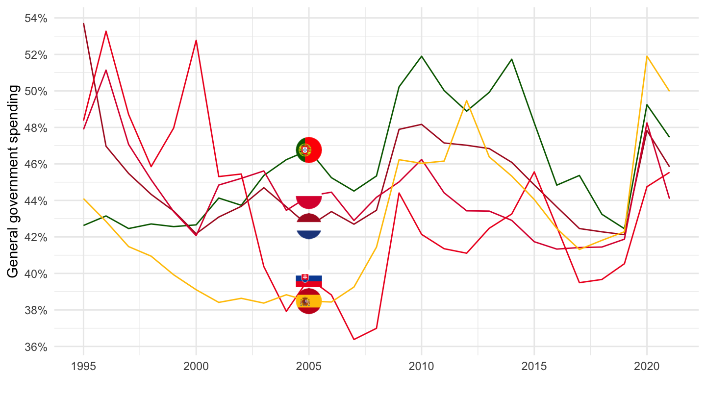

Czech Republic, United Kingdom, Israel, Estonia, Japan

Code

DP_LIVE %>%
  filter(INDICATOR == "GGEXP",
         LOCATION %in% c("CZE", "GBR", "ISR", "EST", "JPN"),
         SUBJECT == "TOT",
         MEASURE == "PC_GDP") %>%
  left_join(DP_LIVE_var$LOCATION, by = "LOCATION") %>%
  year_to_date() %>%
  left_join(colors, by = c("Location" = "country")) %>%
  mutate(obsValue = obsValue/100) %>%
  ggplot(.) + geom_line(aes(x = date, y = obsValue, color = color)) +
  theme_minimal() + xlab("") + ylab("General government spending") +
  add_5flags + scale_color_identity() +
  scale_y_continuous(breaks = 0.01*seq(0, 260, 2),
                     labels = percent_format(accuracy = 1, p = "")) +
  scale_x_date(breaks = as.Date(paste0(seq(1700, 2100, 5), "-01-01")),
               labels = date_format("%Y"))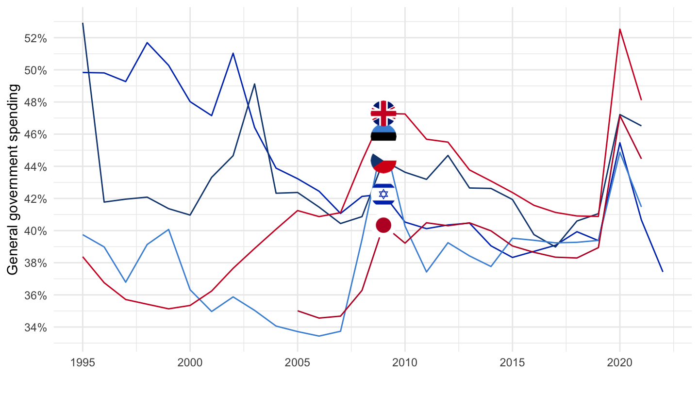

Latvia, United States, Lithuania, Switzerland, Costa Rica

Code

DP_LIVE %>%
  filter(INDICATOR == "GGEXP",
         LOCATION %in% c("LVA", "USA", "LTU", "CHE", "CRI"),
         SUBJECT == "TOT",
         MEASURE == "PC_GDP") %>%
  left_join(DP_LIVE_var$LOCATION, by = "LOCATION") %>%
  year_to_date() %>%
  left_join(colors, by = c("Location" = "country")) %>%
  mutate(obsValue = obsValue/100) %>%
  ggplot(.) + geom_line(aes(x = date, y = obsValue, color = color)) +
  theme_minimal() + xlab("") + ylab("General government spending") +
  add_5flags + scale_color_identity() +
  scale_y_continuous(breaks = 0.01*seq(0, 260, 2),
                     labels = percent_format(accuracy = 1, p = "")) +
  scale_x_date(breaks = as.Date(paste0(seq(1700, 2100, 5), "-01-01")),
               labels = date_format("%Y"))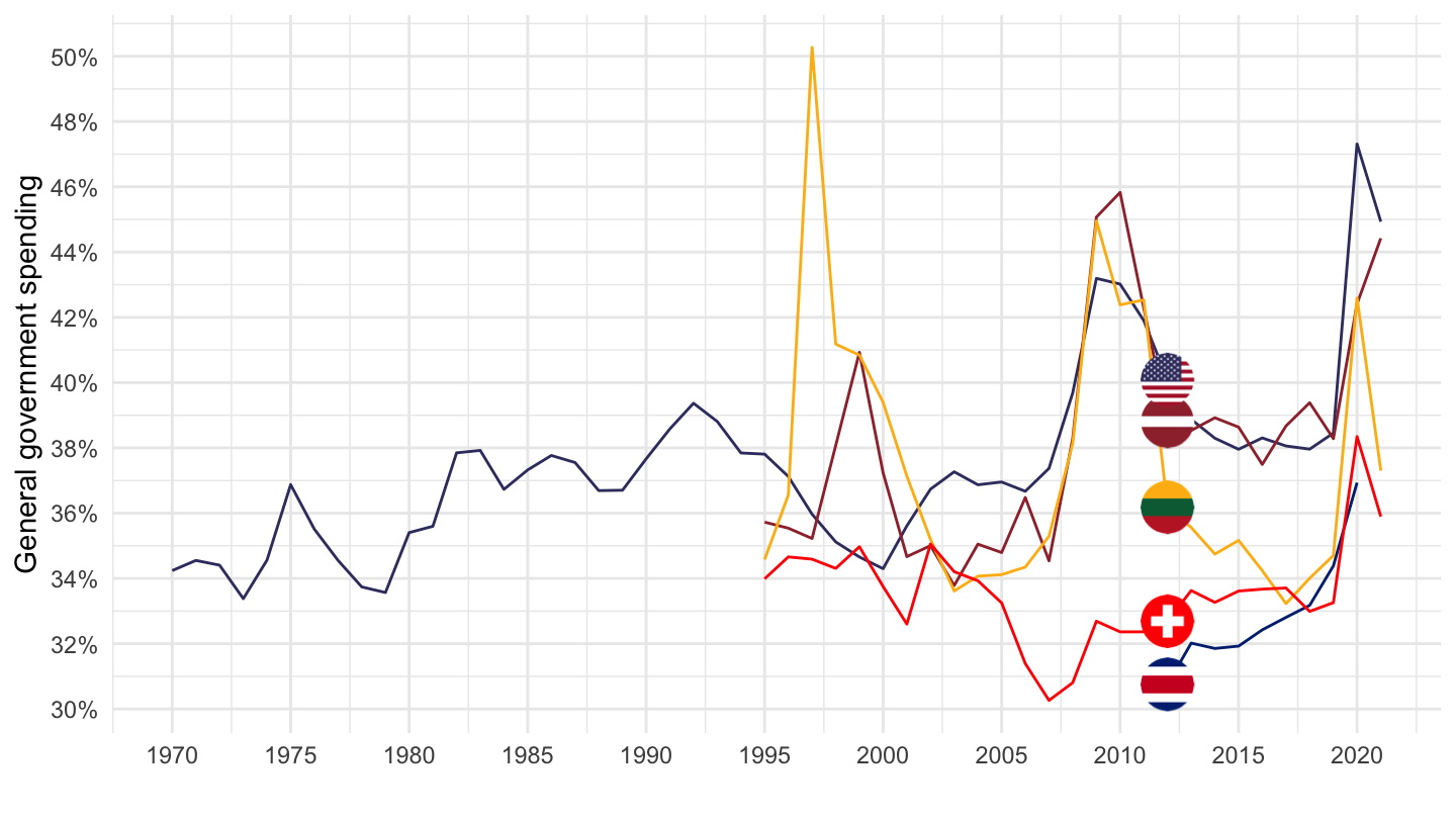

Colombia, Korea, Chile, Ireland

Code

DP_LIVE %>%
  filter(INDICATOR == "GGEXP",
         LOCATION %in% c("COL", "KOR", "CHL", "IRL"),
         SUBJECT == "TOT",
         MEASURE == "PC_GDP") %>%
  left_join(DP_LIVE_var$LOCATION, by = "LOCATION") %>%
  year_to_date() %>%
  left_join(colors, by = c("Location" = "country")) %>%
  mutate(obsValue = obsValue/100) %>%
  ggplot(.) + geom_line(aes(x = date, y = obsValue, color = color)) +
  theme_minimal() + xlab("") + ylab("General government spending") +
  add_4flags + scale_color_identity() +
  scale_y_continuous(breaks = 0.01*seq(0, 260, 2),
                     labels = percent_format(accuracy = 1, p = "")) +
  scale_x_date(breaks = as.Date(paste0(seq(1700, 2100, 5), "-01-01")),
               labels = date_format("%Y"))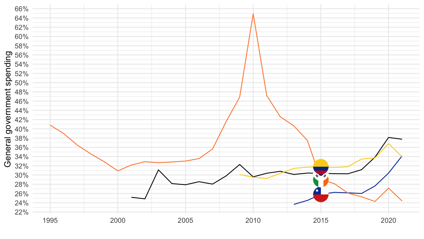

PASSCAR - Passenger car registrations

Table

Code

DP_LIVE %>%
  filter(INDICATOR == "PASSCAR") %>%
  left_join(DP_LIVE_var$LOCATION, by = "LOCATION") %>%
  group_by(LOCATION, Location, FREQUENCY) %>%
  arrange(obsTime) %>%
  summarise(date_min = min(obsTime),
            date_max = max(obsTime)) %>%
  mutate(Flag = gsub(" ", "-", str_to_lower(gsub(" ", "-", Location))),
         Flag = paste0('<img src="../../icon/flag/vsmall/', Flag, '.png" alt="Flag">')) %>%
  select(Flag, everything()) %>%
  {if (is_html_output()) datatable(., filter = 'top', rownames = F, escape = F) else .}

SHPRICE - Share Prices

Table

Code

DP_LIVE %>%
  filter(INDICATOR == "SHPRICE") %>%
  left_join(DP_LIVE_var$LOCATION, by = "LOCATION") %>%
  group_by(LOCATION, Location) %>%
  arrange(obsTime) %>%
  summarise(date_min = min(obsTime),
            date_max = max(obsTime)) %>%
  mutate(Flag = gsub(" ", "-", str_to_lower(gsub(" ", "-", Location))),
         Flag = paste0('<img src="../../icon/flag/vsmall/', Flag, '.png" alt="Flag">')) %>%
  select(Flag, everything()) %>%
  {if (is_html_output()) datatable(., filter = 'top', rownames = F, escape = F) else .}

United States, Europe

Log

Code

DP_LIVE %>%
  filter(INDICATOR == "SHPRICE",
         LOCATION %in% c("EA19", "USA"),
         FREQUENCY == "M") %>%
  left_join(DP_LIVE_var$LOCATION, by = "LOCATION") %>%
  mutate(Location = ifelse(LOCATION == "EA19", "Europe", Location)) %>%
  year_to_date() %>%
  filter(date >= as.Date("2001-01-01")) %>%
  group_by(LOCATION) %>%
  mutate(obsValue = 100*obsValue/obsValue[1]) %>%
  left_join(colors, by = c("Location" = "country")) %>%
  mutate(color = ifelse(LOCATION == "USA", color2, color)) %>%
  ggplot(.) + geom_line(aes(x = date, y = obsValue, color = color)) +
  theme_minimal() + xlab("") + ylab("Share Prices") +
  add_2flags + scale_color_identity() +
  scale_y_log10(breaks = seq(0, 260, 20),
                     labels = scales::dollar_format(accuracy = 1, p = "")) +
  scale_x_date(breaks = as.Date(paste0(seq(2001, 2027, 2), "-01-01")),
               labels = date_format("%Y"))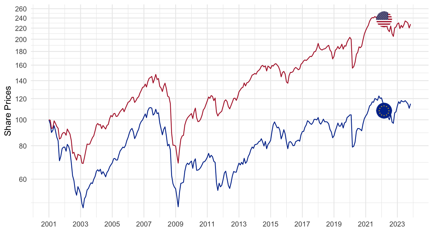

Linear

Code

DP_LIVE %>%
  filter(INDICATOR == "SHPRICE",
         LOCATION %in% c("EA19", "USA"),
         FREQUENCY == "M") %>%
  left_join(DP_LIVE_var$LOCATION, by = "LOCATION") %>%
  mutate(Location = ifelse(LOCATION == "EA19", "Europe", Location)) %>%
  year_to_date() %>%
  filter(date >= as.Date("2001-01-01")) %>%
  group_by(LOCATION) %>%
  mutate(obsValue = 100*obsValue/obsValue[1]) %>%
  left_join(colors, by = c("Location" = "country")) %>%
  mutate(color = ifelse(LOCATION == "USA", color2, color)) %>%
  ggplot(.) + geom_line(aes(x = date, y = obsValue, color = color)) +
  theme_minimal() + xlab("") + ylab("Share Prices") +
  add_2flags + scale_color_identity() +
  scale_y_continuous(breaks = seq(0, 260, 20),
                     labels = scales::dollar_format(accuracy = 1, p = "")) +
  scale_x_date(breaks = as.Date(paste0(seq(2001, 2027, 2), "-01-01")),
               labels = date_format("%Y"))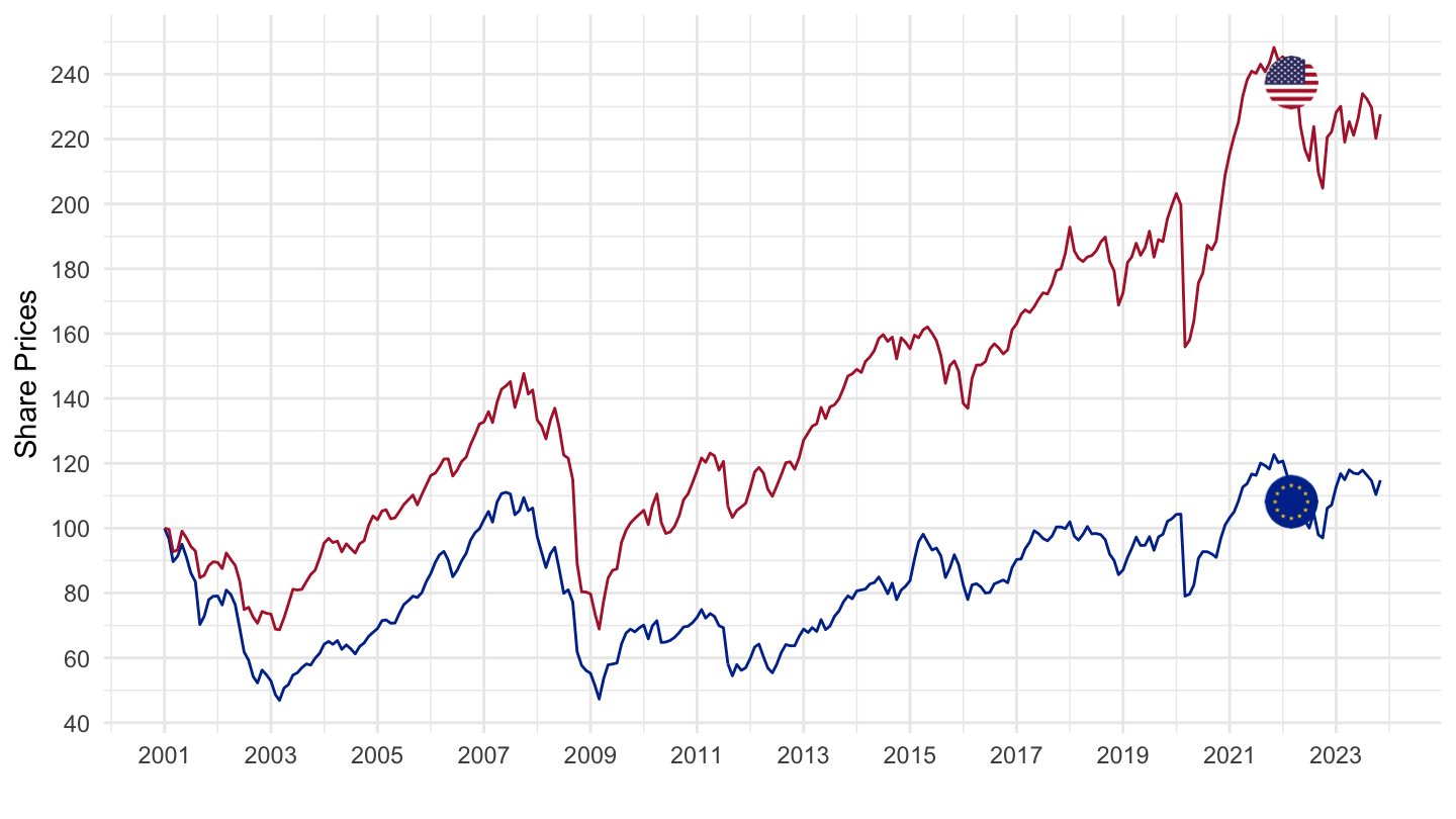

HHDEBT - Household Debt

Table

Code

DP_LIVE %>%
  filter(INDICATOR == "HHDEBT") %>%
  left_join(DP_LIVE_var$LOCATION, by = "LOCATION") %>%
  group_by(LOCATION, Location) %>%
  arrange(obsTime) %>%
  summarise(date_min = min(obsTime),
            date_max = max(obsTime)) %>%
  arrange(as.numeric(date_min), -as.numeric(date_max)) %>%
  mutate(Flag = gsub(" ", "-", str_to_lower(gsub(" ", "-", Location))),
         Flag = paste0('<img src="../../icon/flag/vsmall/', Flag, '.png" alt="Flag">')) %>%
  select(Flag, everything()) %>%
  {if (is_html_output()) datatable(., filter = 'top', rownames = F, escape = F) else .}

France, Germany, Japan

Code

DP_LIVE %>%
  filter(LOCATION %in% c("FRA", "DEU", "JPN"),
         INDICATOR == "HHDEBT") %>%
  year_to_date %>%
  left_join(DP_LIVE_var$LOCATION, by = "LOCATION") %>%
  group_by(LOCATION) %>%
  left_join(colors, by = c("Location" = "country")) %>%
  mutate(obsValue = obsValue / 100) %>%
  ggplot(.) + geom_line(aes(x = date, y = obsValue, color = color)) + 
  scale_color_identity() + add_3flags +
  theme_minimal() + xlab("") + ylab("Household Debt (% of net disposable income)") +
  scale_x_date(breaks = seq(1940, 2020, 5) %>% paste0("-01-01") %>% as.Date,
               labels = date_format("%Y")) +
  scale_y_continuous(breaks = 0.01*seq(-10, 200, 5),
                     labels = percent_format(accuracy = 1, prefix = "")) +
  theme(legend.position = c(0.2, 0.90),
        legend.title = element_blank())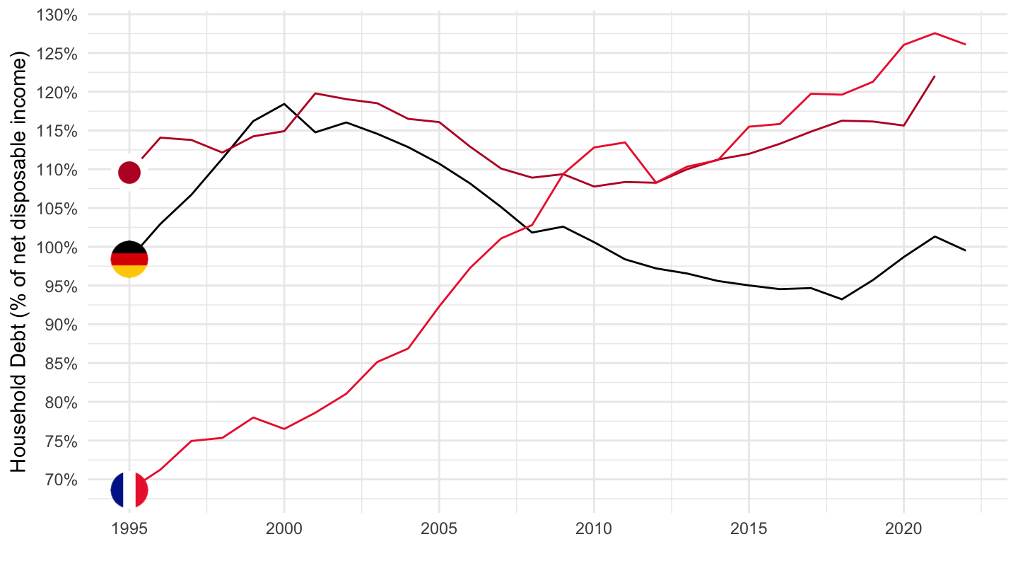

Canada, Denmark, Finland

Code

DP_LIVE %>%
  filter(LOCATION %in% c("CAN", "DNK", "FIN"),
         INDICATOR == "HHDEBT") %>%
  year_to_date %>%
  left_join(DP_LIVE_var$LOCATION, by = "LOCATION") %>%
  group_by(LOCATION) %>%
  left_join(colors, by = c("Location" = "country")) %>%
  mutate(obsValue = obsValue / 100) %>%
  ggplot(.) + geom_line(aes(x = date, y = obsValue, color = color)) + 
  scale_color_identity() + add_3flags +
  theme_minimal() + xlab("") + ylab("Household Debt (% of net disposable income)") +
  scale_x_date(breaks = seq(1940, 2020, 5) %>% paste0("-01-01") %>% as.Date,
               labels = date_format("%Y")) +
  scale_y_continuous(breaks = 0.01*seq(-10, 400, 10),
                     labels = percent_format(accuracy = 1, prefix = "")) +
  theme(legend.position = c(0.2, 0.90),
        legend.title = element_blank())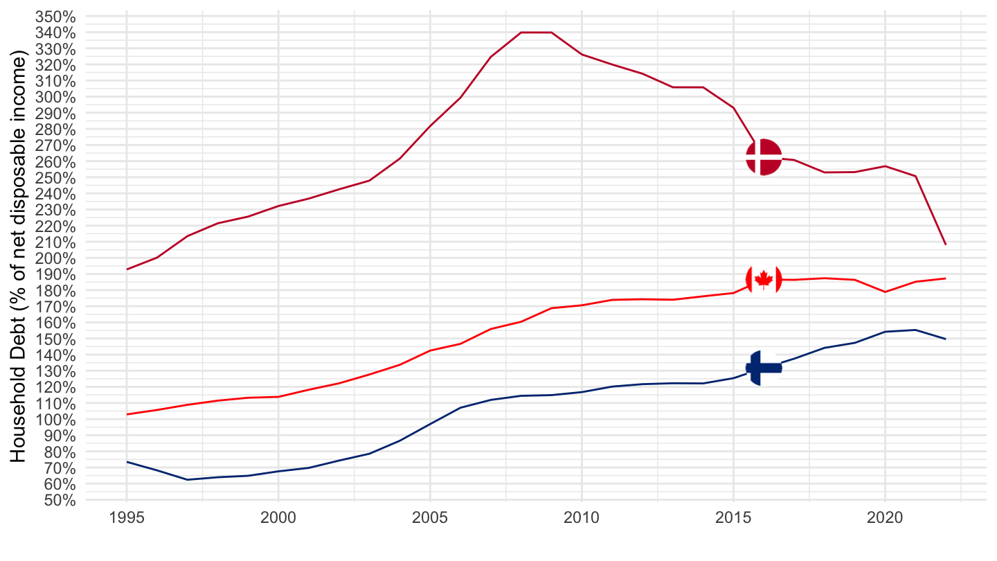

Japan, United Kingdom, United States

Code

DP_LIVE %>%
  filter(LOCATION %in% c("JPN", "GBR", "USA"),
         INDICATOR == "HHDEBT") %>%
  year_to_date %>%
  left_join(DP_LIVE_var$LOCATION, by = "LOCATION") %>%
  group_by(LOCATION) %>%
  left_join(colors, by = c("Location" = "country")) %>%
  mutate(obsValue = obsValue / 100) %>%
  ggplot(.) + geom_line(aes(x = date, y = obsValue, color = color)) + 
  scale_color_identity() + add_3flags +
  theme_minimal() + xlab("") + ylab("Household Debt (% of net disposable income)") +
  scale_x_date(breaks = seq(1940, 2020, 5) %>% paste0("-01-01") %>% as.Date,
               labels = date_format("%Y")) +
  scale_y_continuous(breaks = 0.01*seq(-10, 400, 10),
                     labels = percent_format(accuracy = 1, prefix = "")) +
  theme(legend.position = c(0.2, 0.90),
        legend.title = element_blank())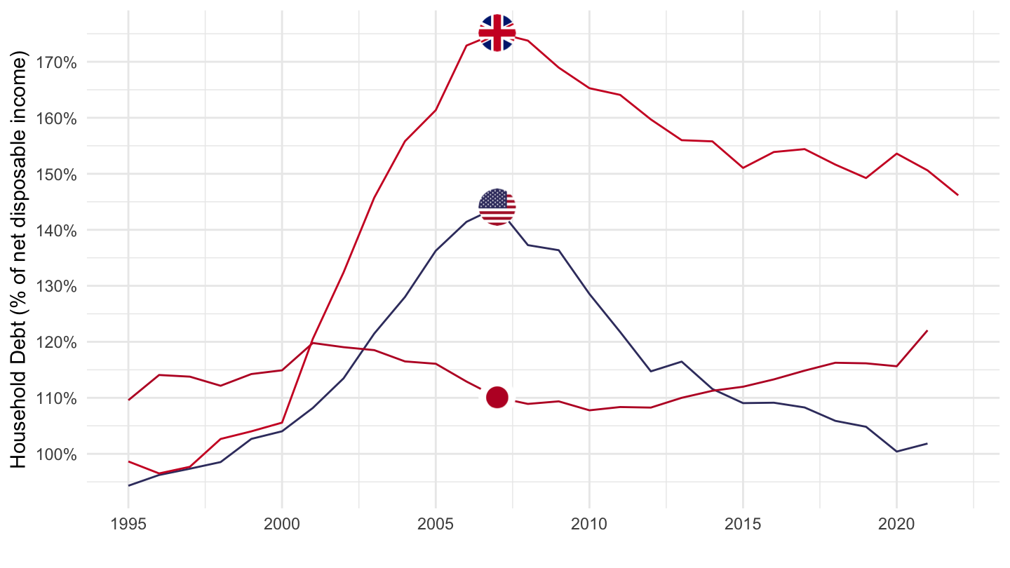

GDPHRWKD - GDP Per hour worked

USD (constant prices 2010 and PPPs)

Table

Code

DP_LIVE %>%
  filter(INDICATOR == "GDPHRWKD") %>%
  left_join(DP_LIVE_var$LOCATION, by = "LOCATION") %>%
  group_by(LOCATION, Location, MEASURE) %>%
  arrange(obsTime) %>%
  summarise(date_min = min(obsTime),
            date_max = max(obsTime)) %>%
  mutate(Flag = gsub(" ", "-", str_to_lower(gsub(" ", "-", Location))),
         Flag = paste0('<img src="../../icon/flag/vsmall/', Flag, '.png" alt="Flag">')) %>%
  select(Flag, everything()) %>%
  {if (is_html_output()) datatable(., filter = 'top', rownames = F, escape = F) else .}

5 countries, IDX2010

Code

DP_LIVE %>%
  filter(INDICATOR == "GDPHRWKD",
         LOCATION %in% c("GBR", "USA", "FRA", "JPN", "ITA"),
         MEASURE == "IDX2010") %>%
  left_join(DP_LIVE_var$LOCATION, by = "LOCATION") %>%
  year_to_date() %>%
  left_join(colors, by = c("Location" = "country")) %>%
  ggplot(.) + theme_minimal() + xlab("") + ylab("Average Wages") +
  geom_line(aes(x = date, y = obsValue, color = color, linetype = Location)) +
  #scale_linetype_manual(values = c("dotted", "solid", "longdash","solid",  "solid")) +
  add_5flags + scale_color_identity() +
  theme(legend.position = c(0.2, 0.85),
        legend.title = element_blank()) +
  scale_y_continuous(breaks = seq(0, 260, 5),
                     labels = scales::dollar_format(accuracy = 1, p = "", su = "")) +
  scale_x_date(breaks = as.Date(paste0(seq(1700, 2020, 5), "-01-01")),
               labels = date_format("%Y"))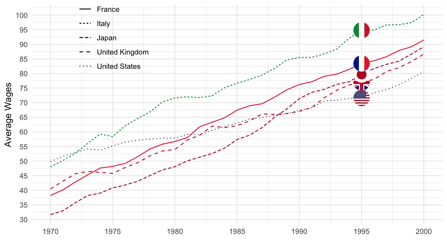

U.S. Dollars

UK, US, France, Japan, Italy

Code

DP_LIVE %>%
  filter(INDICATOR == "GDPHRWKD",
         LOCATION %in% c("GBR", "USA", "FRA", "JPN", "ITA"),
         MEASURE == "USD") %>%
  left_join(DP_LIVE_var$LOCATION, by = "LOCATION") %>%
  year_to_date() %>%
  left_join(colors, by = c("Location" = "country")) %>%
  mutate(color = ifelse(LOCATION == "FRA", color2, color)) %>%
  ggplot(.) + theme_minimal() + xlab("") + ylab("Average Wages") +
  geom_line(aes(x = date, y = obsValue, color = color, linetype = Location)) +
  #scale_linetype_manual(values = c("dotted", "solid", "longdash","solid",  "solid")) +
  add_5flags + scale_color_identity() +
  theme(legend.position = c(0.2, 0.85),
        legend.title = element_blank()) +
  scale_y_continuous(breaks = seq(0, 260, 5),
                     labels = scales::dollar_format(accuracy = 1, p = "$", su = "")) +
  scale_x_date(breaks = as.Date(paste0(seq(1700, 2020, 5), "-01-01")),
               labels = date_format("%Y"))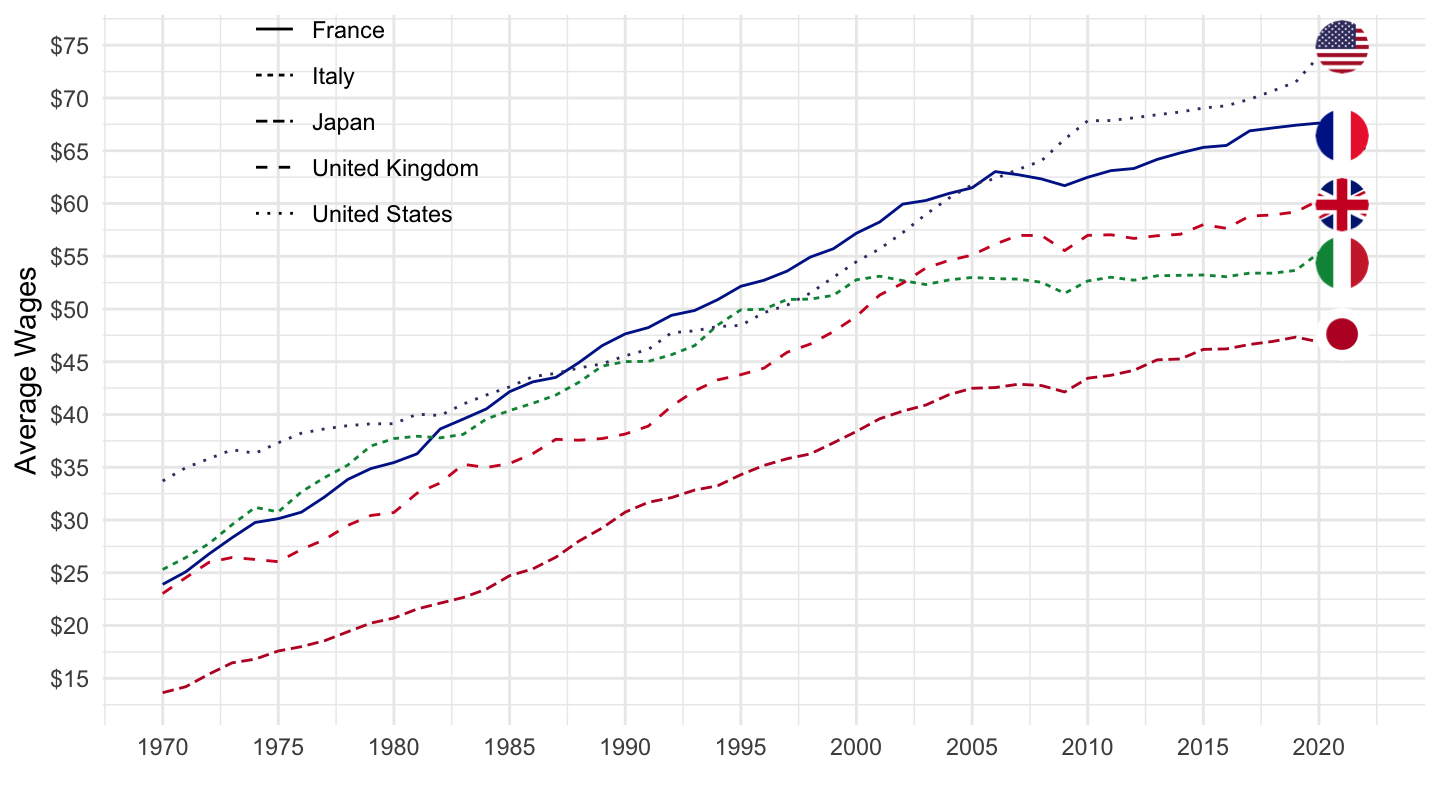

Greece, UK

Code

DP_LIVE %>%
  filter(INDICATOR == "GDPHRWKD",
         LOCATION %in% c("GRC", "GBR"),
         MEASURE == "USD") %>%
  left_join(DP_LIVE_var$LOCATION, by = "LOCATION") %>%
  mutate(Location = ifelse(LOCATION == "EA19", "Europe", Location)) %>%
  year_to_date() %>%
  filter(date >= as.Date("1990-01-01")) %>%
  ggplot(.) + theme_minimal() + xlab("") + ylab("GDP Per Hour Worked (Source: OECD)") +
  add_2flags +
  geom_line(aes(x = date, y = obsValue, color = Location)) +
  scale_color_manual(values = c("#0D5EAF", "#CF142B")) +
  theme(legend.position = c(0.2, 0.85),
        legend.title = element_blank()) +
  scale_y_log10(breaks = seq(0, 260, 5),
                     labels = scales::dollar_format(accuracy = 1, p = "$")) +
  scale_x_date(breaks = as.Date(paste0(seq(1700, 2020, 5), "-01-01")),
               labels = date_format("%Y"))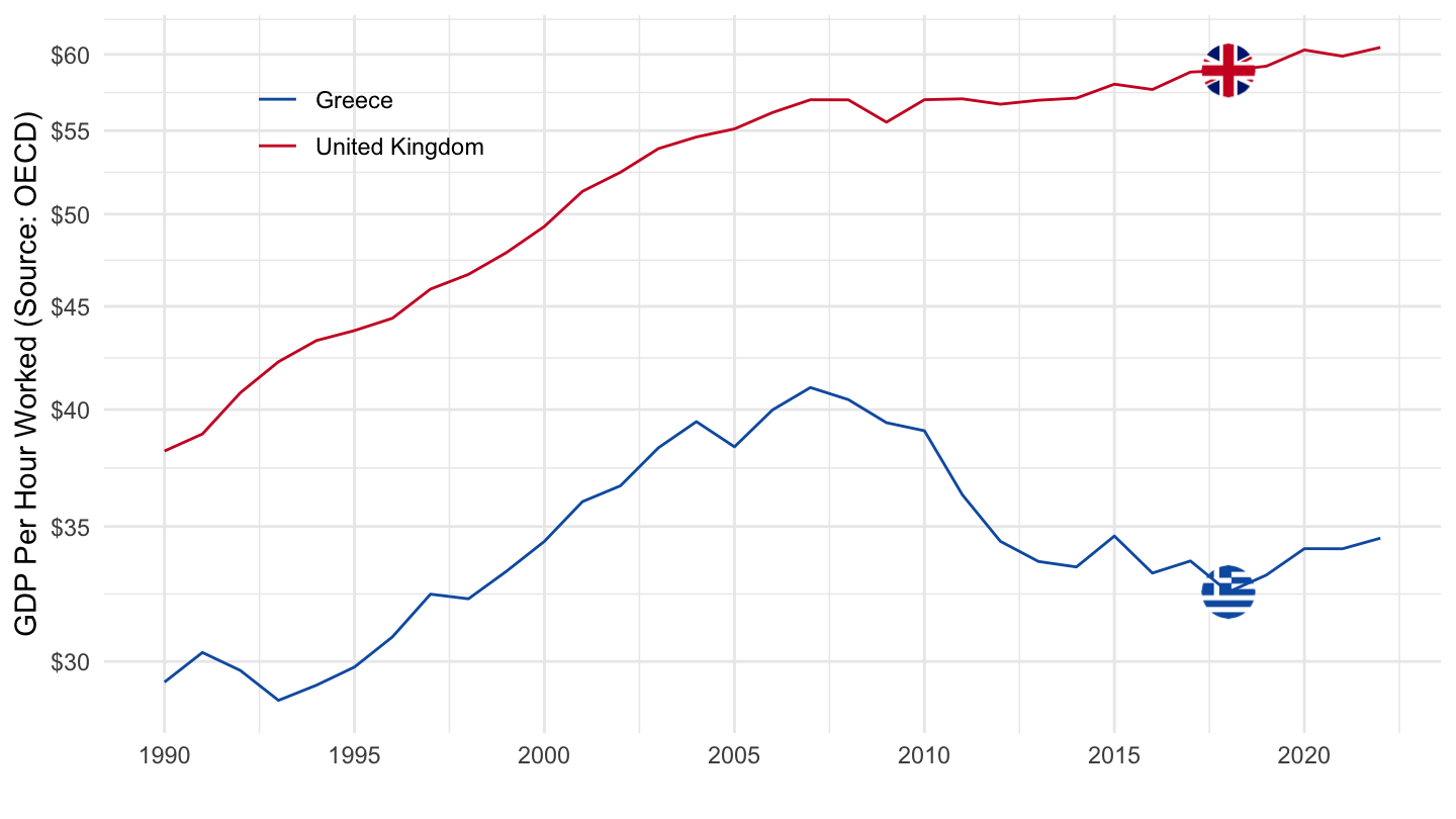

Greece, UK, Italy

Code

DP_LIVE %>%
  filter(INDICATOR == "GDPHRWKD",
         LOCATION %in% c("GRC", "GBR", "ITA"),
         MEASURE == "USD") %>%
  left_join(DP_LIVE_var$LOCATION, by = "LOCATION") %>%
  mutate(Location = ifelse(LOCATION == "EA19", "Europe", Location)) %>%
  year_to_date() %>%
  filter(date >= as.Date("1990-01-01")) %>%
  ggplot(.) + theme_minimal() + xlab("") + ylab("GDP Per Hour Worked (Source: OECD)") +
  add_3flags +
  geom_line(aes(x = date, y = obsValue, color = Location)) +
  scale_color_manual(values = c("#0D5EAF", "#009246", "#CF142B")) +
  scale_linetype_manual(values = c("solid", "solid", "longdash","solid",  "solid")) +
  theme(legend.position = c(0.2, 0.9),
        legend.title = element_blank()) +
  scale_y_log10(breaks = seq(0, 260, 5),
                     labels = scales::dollar_format(accuracy = 1, p = "$")) +
  scale_x_date(breaks = as.Date(paste0(seq(1700, 2020, 5), "-01-01")),
               labels = date_format("%Y"))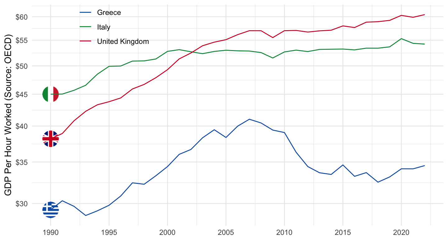

AVWAGE - General government debt

Table

Code

DP_LIVE %>%
  filter(INDICATOR == "AVWAGE") %>%
  left_join(DP_LIVE_var$LOCATION, by = "LOCATION") %>%
  group_by(LOCATION, Location) %>%
  arrange(obsTime) %>%
  summarise(date_min = min(obsTime),
            date_max = max(obsTime)) %>%
  mutate(Flag = gsub(" ", "-", str_to_lower(gsub(" ", "-", Location))),
         Flag = paste0('<img src="../../icon/flag/vsmall/', Flag, '.png" alt="Flag">')) %>%
  select(Flag, everything()) %>%
  {if (is_html_output()) datatable(., filter = 'top', rownames = F, escape = F) else .}

5 countries

Code

DP_LIVE %>%
  filter(INDICATOR == "AVWAGE",
         LOCATION %in% c("GBR", "USA", "FRA", "JPN", "ITA")) %>%
  left_join(DP_LIVE_var$LOCATION, by = "LOCATION") %>%
  year_to_date() %>%
  ggplot(.) + theme_minimal() + xlab("") + ylab("Average Wages") +
  geom_line(aes(x = date, y = obsValue / 1000, color = Location, linetype = Location)) +
  scale_color_manual(values = c("#000000", "#009246", "#BC002D", "#6E82B5", "#B22234")) +
  scale_linetype_manual(values = c("solid", "solid", "longdash","solid",  "solid")) +
  geom_image(data = . %>%
               filter(date == as.Date("1990-01-01")) %>%
               mutate(date = as.Date("1990-01-01"),
                      image = paste0("../../icon/flag/", str_to_lower(gsub(" ", "-", Location)), ".png")),
             aes(x = date, y = obsValue/1000, image = image), asp = 1.5) +
  theme(legend.position = c(0.2, 0.85),
        legend.title = element_blank()) +
  scale_y_continuous(breaks = seq(0, 260, 5),
                     labels = scales::dollar_format(accuracy = 1, p = "$", su = "k")) +
  scale_x_date(breaks = as.Date(paste0(seq(1700, 2020, 5), "-01-01")),
               labels = date_format("%Y"))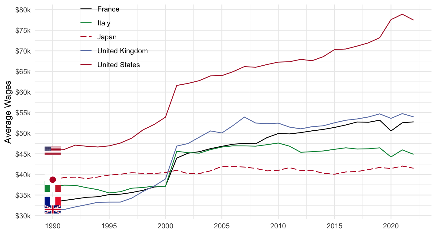

GGDEBT - General government debt

Table

Code

DP_LIVE %>%
  filter(INDICATOR == "GGDEBT") %>%
  left_join(DP_LIVE_var$LOCATION, by = "LOCATION") %>%
  group_by(LOCATION, Location) %>%
  arrange(obsTime) %>%
  summarise(date_min = min(obsTime),
            date_max = max(obsTime)) %>%
  mutate(Flag = gsub(" ", "-", str_to_lower(gsub(" ", "-", Location))),
         Flag = paste0('<img src="../../icon/flag/vsmall/', Flag, '.png" alt="Flag">')) %>%
  select(Flag, everything()) %>%
  {if (is_html_output()) datatable(., filter = 'top', rownames = F, escape = F) else .}

5 countries

Code

DP_LIVE %>%
  filter(INDICATOR == "GGDEBT",
         LOCATION %in% c("GBR", "USA", "FRA", "JPN", "ITA")) %>%
  left_join(DP_LIVE_var$LOCATION, by = "LOCATION") %>%
  year_to_date() %>%
  ggplot(.) + theme_minimal() + xlab("") + ylab("Government Debt (% of GDP)") +
  geom_line(aes(x = date, y = obsValue / 100, color = Location, linetype = Location)) +
  scale_color_manual(values = c("#000000", "#009246", "#BC002D", "#6E82B5", "#B22234")) +
  scale_linetype_manual(values = c("solid", "solid", "longdash","solid",  "solid")) +
  geom_image(data = . %>%
               filter(date == as.Date("1997-01-01")) %>%
               mutate(date = as.Date("1997-01-01"),
                      image = paste0("../../icon/flag/", str_to_lower(gsub(" ", "-", Location)), ".png")),
             aes(x = date, y = obsValue/100, image = image), asp = 1.5) +
  theme(legend.position = c(0.2, 0.85),
        legend.title = element_blank()) +
  scale_y_continuous(breaks = 0.01*seq(0, 260, 20),
                     labels = scales::percent_format(accuracy = 1)) +
  scale_x_date(breaks = as.Date(paste0(seq(1700, 2020, 5), "-01-01")),
               labels = date_format("%Y"))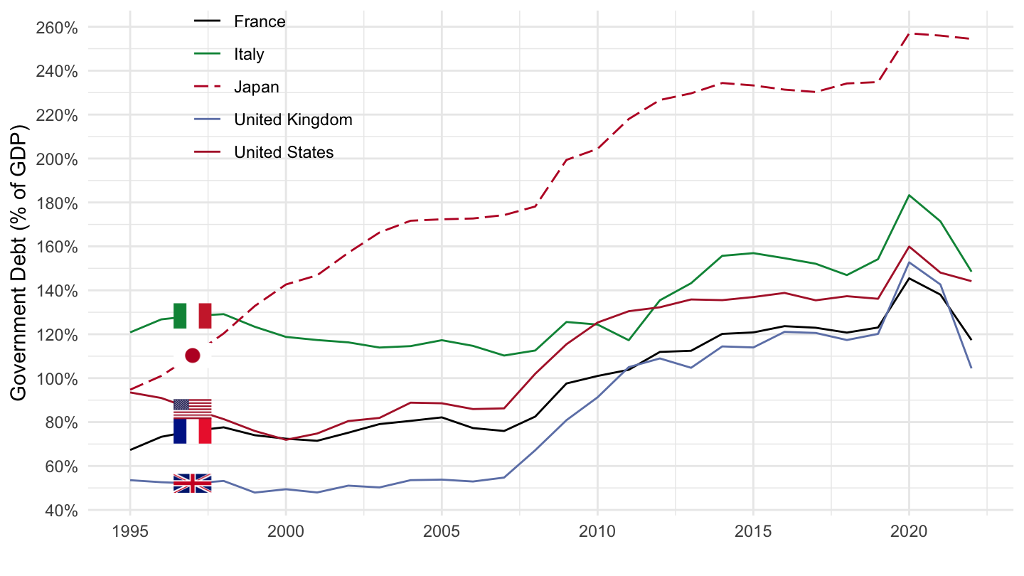

5 countries

Code

DP_LIVE %>%
  filter(INDICATOR == "GGDEBT",
         LOCATION %in% c("GBR", "USA", "DEU", "JPN", "ITA", "FRA")) %>%
  left_join(DP_LIVE_var$LOCATION, by = "LOCATION") %>%
  year_to_date() %>%
  left_join(colors, by = c("Location" = "country")) %>%
  mutate(obsValue = obsValue/100) %>%
  ggplot(.) + theme_minimal() + xlab("") + ylab("Dette publique (années de PIB)") +
  geom_line(aes(x = date, y = obsValue, color = color)) +
  scale_color_identity() + add_6flags +
  scale_linetype_manual(values = c("solid", "solid", "longdash","solid",  "solid")) +
  theme(legend.position = c(0.2, 0.85),
        legend.title = element_blank()) +
  scale_y_continuous(breaks = 0.01*seq(0, 260, 20),
                     labels = scales::dollar_format(acc = .1, pre = "", su = " années")) +
  scale_x_date(breaks = as.Date(paste0(seq(1700, 2020, 5), "-01-01")),
               labels = date_format("%Y"))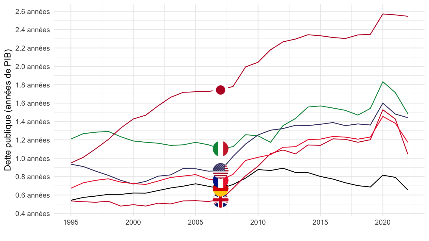

Labour force participation rate

Table, 2019

Code

DP_LIVE %>%
  filter(obsTime == "2019",
         INDICATOR == "LFPR") %>%
  select(LOCATION, SUBJECT, obsValue) %>%
  left_join(DP_LIVE_var$LOCATION, by = "LOCATION") %>%
  mutate(obsValue = round(obsValue, 1)) %>%
  spread(SUBJECT, obsValue) %>%
  mutate(Flag = gsub(" ", "-", str_to_lower(gsub(" ", "-", Location))),
         Flag = paste0('<img src="../../icon/flag/vsmall/', Flag, '.png" alt="Flag">')) %>%
  select(Flag, everything()) %>%
  {if (is_html_output()) datatable(., filter = 'top', rownames = F, escape = F) else .}

Netherlands, Germany, Japan

Code

DP_LIVE %>%
  filter(LOCATION %in% c("DEU", "JPN", "NLD"), 
         INDICATOR == "LFPR",
         SUBJECT == "15_64") %>%
  left_join(DP_LIVE_var$LOCATION, by = "LOCATION") %>%
  year_to_date() %>%
  ggplot() + geom_line(aes(x = date, y = obsValue/100, color = Location)) +
  scale_color_manual(values = c("#000000", "#BC002D", "#21468B")) +
  theme_minimal() +
  scale_x_date(breaks = seq(1920, 2025, 5) %>% paste0("-01-01") %>% as.Date,
               labels = date_format("%Y")) +
  theme(legend.position = c(0.15, 0.8),
        legend.title = element_blank()) +
  scale_y_continuous(breaks = 0.01*seq(-6, 90, 2),
                     labels = percent_format(accuracy = 1)) +
  ylab("Labour force participation rate") + xlab("")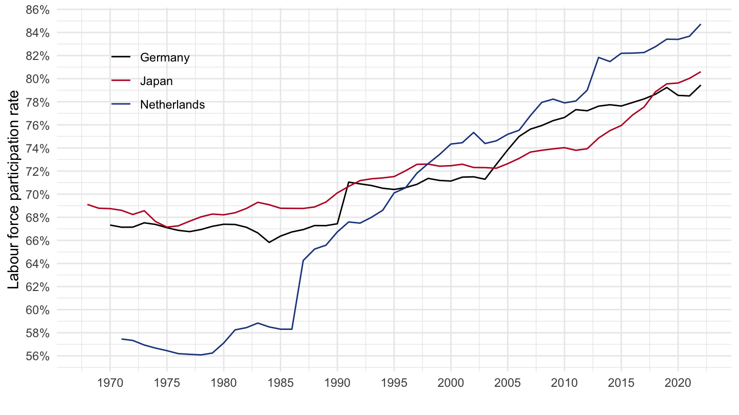

Employment Rates

Netherlands, Germany, Japan

Code

DP_LIVE %>%
  filter(LOCATION %in% c("DEU", "JPN", "NLD"), 
         INDICATOR == "EMP", 
         SUBJECT == "TOT",
         MEASURE == "PC_WKGPOP") %>%
  left_join(DP_LIVE_var$LOCATION, by = "LOCATION") %>%
  year_to_date() %>%
  mutate(obsValue = obsValue/100) %>%
  ggplot() + geom_line(aes(x = date, y = obsValue, color = Location)) +
  scale_color_manual(values = c("#000000", "#BC002D", "#21468B")) +
  theme_minimal() +
  scale_x_date(breaks = seq(1920, 2025, 2) %>% paste0("-01-01") %>% as.Date,
               labels = date_format("%Y")) +
  theme(legend.position = c(0.15, 0.8),
        legend.title = element_blank()) +
  scale_y_continuous(breaks = 0.01*seq(-6, 90, 2),
                     labels = percent_format(accuracy = 1)) +
  ylab("Employment rates") + xlab("")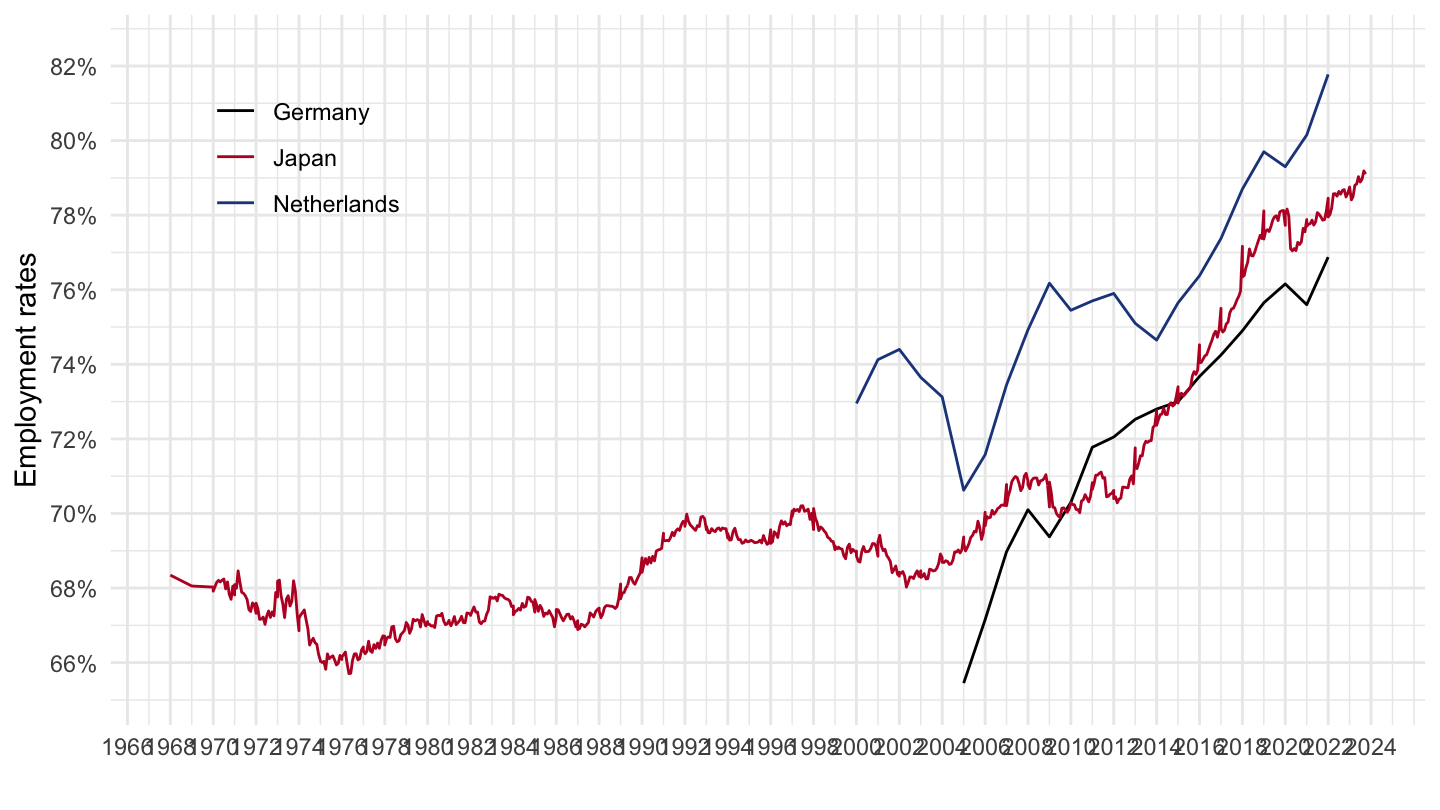

France, Italy, Spain

Code

DP_LIVE %>%
  filter(LOCATION %in% c("FRA", "ITA", "ESP"), 
         INDICATOR == "EMP", 
         SUBJECT == "TOT",
         MEASURE == "PC_WKGPOP") %>%
  left_join(DP_LIVE_var$LOCATION, by = "LOCATION") %>%
  year_to_date() %>%
  mutate(obsValue = obsValue/100) %>%
  ggplot() + geom_line(aes(x = date, y = obsValue, color = Location)) +
  scale_color_manual(values = c("#002395", "#009246", "#C60B1E")) +
  theme_minimal() +
  scale_x_date(breaks = seq(1920, 2025, 2) %>% paste0("-01-01") %>% as.Date,
               labels = date_format("%Y")) +
  theme(legend.position = c(0.15, 0.8),
        legend.title = element_blank()) +
  scale_y_continuous(breaks = 0.01*seq(-6, 90, 2),
                     labels = percent_format(accuracy = 1)) +
  ylab("Part-time employment rate") + xlab("")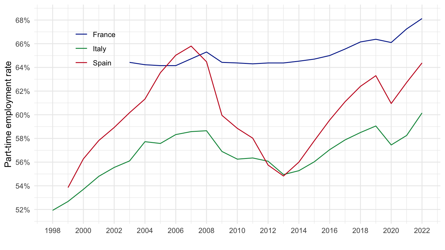

Gross Pension Replacement Rates

Men

Code

DP_LIVE %>%
  filter(LOCATION %in% c("DEU", "FRA", "SWE"), 
         INDICATOR == "GPENSION", 
         SUBJECT == "MEN") %>%
  left_join(DP_LIVE_var$LOCATION %>%
              setNames(c("LOCATION", "Location")), by = "LOCATION") %>%
  year_to_date() %>%
  mutate(obsValue = obsValue/100) %>%
  ggplot() + geom_line(aes(x = date, y = obsValue, color = Location)) +
  scale_color_manual(values = c("#ED2939", "#000000", "#006AA7")) +
  theme_minimal() +
  scale_x_date(breaks = seq(1920, 2025, 1) %>% paste0("-01-01") %>% as.Date,
               labels = date_format("%Y")) +
  theme(legend.position = c(0.35, 0.3),
        legend.title = element_blank()) +
  scale_y_continuous(breaks = 0.01*seq(-6, 90, 2),
                     labels = percent_format(accuracy = 1)) +
  ylab("Gross Pension Replacement Rate") + xlab("")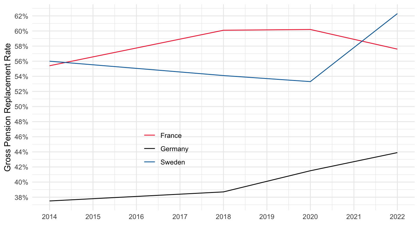

Women

Code

DP_LIVE %>%
  filter(LOCATION %in% c("DEU", "FRA", "SWE"), 
         INDICATOR == "GPENSION", 
         SUBJECT == "WOMEN") %>%
  left_join(DP_LIVE_var$LOCATION %>%
              setNames(c("LOCATION", "Location")), by = "LOCATION") %>%
  year_to_date() %>%
  mutate(obsValue = obsValue/100) %>%
  ggplot() + geom_line(aes(x = date, y = obsValue, color = Location)) +
  scale_color_manual(values = c("#ED2939", "#000000", "#006AA7")) +
  theme_minimal() +
  scale_x_date(breaks = seq(1920, 2025, 1) %>% paste0("-01-01") %>% as.Date,
               labels = date_format("%Y")) +
  theme(legend.position = c(0.35, 0.3),
        legend.title = element_blank()) +
  scale_y_continuous(breaks = 0.01*seq(-6, 90, 2),
                     labels = percent_format(accuracy = 1)) +
  ylab("Gross Pension Replacement Rate") + xlab("")

INPROD

Just Manufacturing

Japan, United Kingdom, USA

Code

DP_LIVE %>%
  filter(LOCATION %in% c("JPN", "GBR", "USA"),
         INDICATOR == "INDPROD",
         SUBJECT == "MFG",
         FREQUENCY == "M") %>%
  month_to_date %>%
  left_join(DP_LIVE_var$LOCATION, by = "LOCATION") %>%
  group_by(LOCATION) %>%
  left_join(colors, by = c("Location" = "country")) %>%
  ggplot(.) + geom_line(aes(x = date, y = obsValue, color = color)) + 
  scale_color_identity() + add_3flags +
  theme_minimal() + xlab("") + ylab("Industrial Production") +
  scale_x_date(breaks = seq(1940, 2020, 5) %>% paste0("-01-01") %>% as.Date,
               labels = date_format("%Y")) +
  scale_y_log10(breaks = seq(-10, 400, 10))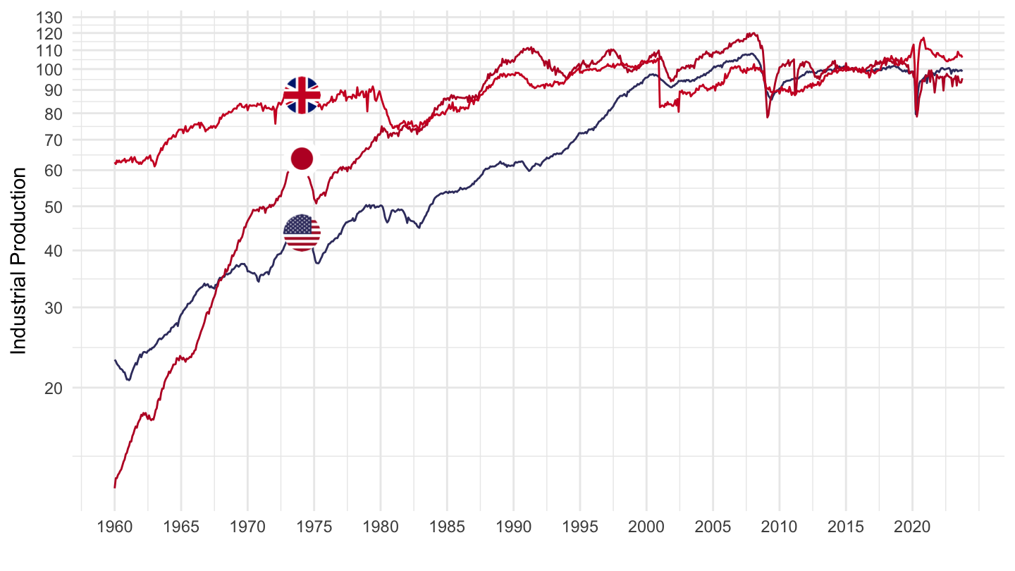

Spain, Italy, France, Germany

All

Code

DP_LIVE %>%
  filter(LOCATION %in% c("ESP", "ITA", "FRA", "DEU"),
         INDICATOR == "INDPROD",
         SUBJECT == "MFG",
         FREQUENCY == "M") %>%
  month_to_date %>%
  left_join(DP_LIVE_var$LOCATION, by = "LOCATION") %>%
  group_by(LOCATION) %>%
  left_join(colors, by = c("Location" = "country")) %>%
  ggplot(.) + geom_line(aes(x = date, y = obsValue, color = color)) + 
  scale_color_identity() + add_4flags +
  theme_minimal() + xlab("") + ylab("Industrial Production") +
  scale_x_date(breaks = seq(1940, 2020, 5) %>% paste0("-01-01") %>% as.Date,
               labels = date_format("%Y")) +
  scale_y_log10(breaks = seq(-10, 400, 10))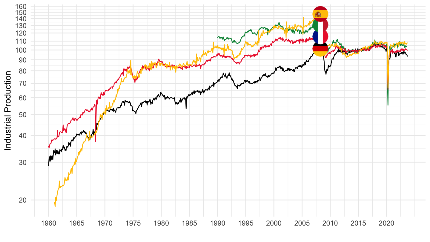

1990-

Code

DP_LIVE %>%
  filter(LOCATION %in% c("ESP", "ITA", "FRA", "DEU"),
         INDICATOR == "INDPROD",
         SUBJECT == "MFG",
         FREQUENCY == "M") %>%
  month_to_date %>%
  filter(date >= as.Date("1990-01-01")) %>%
  left_join(DP_LIVE_var$LOCATION, by = "LOCATION") %>%
  group_by(LOCATION) %>%
  arrange(date) %>%
  mutate(obsValue = 100*obsValue/obsValue[1]) %>%
  left_join(colors, by = c("Location" = "country")) %>%
  ggplot(.) + geom_line(aes(x = date, y = obsValue, color = color)) + 
  scale_color_identity() + add_4flags +
  theme_minimal() + xlab("") + ylab("Industrial Production") +
  scale_x_date(breaks = seq(1940, 2020, 5) %>% paste0("-01-01") %>% as.Date,
               labels = date_format("%Y")) +
  scale_y_log10(breaks = seq(-10, 400, 10))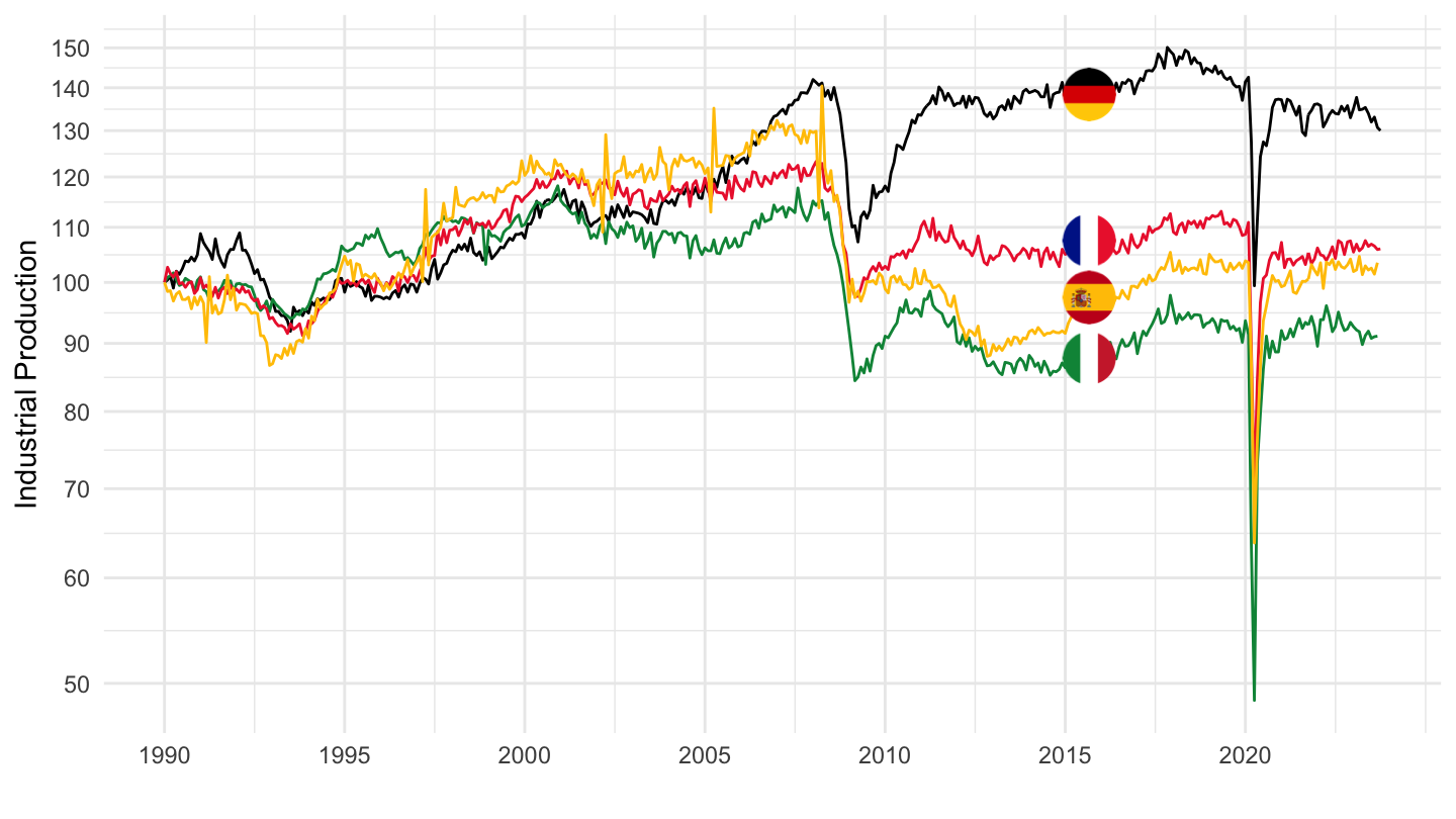

Germany

All

Code

DP_LIVE %>%
  filter(INDICATOR == "INDPROD", 
         LOCATION == "DEU", 
         FREQUENCY == "M") %>%
  left_join(DP_LIVE_var$SUBJECT, by = "SUBJECT") %>%
  month_to_date %>%
  ggplot + geom_line(aes(x = date, y = obsValue, color = Subject))+ 
  theme_minimal() + xlab("") + ylab("Industrial Production, Index") +
  scale_x_date(breaks = seq(1960, 2020, 5) %>% paste0("-01-01") %>% as.Date,
               labels = date_format("%Y")) +
  scale_y_log10(breaks = seq(-10, 200, 10),
                     labels = dollar_format(accuracy = 1, prefix = "")) +
  scale_color_manual(values = viridis(5)[1:4]) +
  theme(legend.position = c(0.8, 0.20),
        legend.title = element_blank())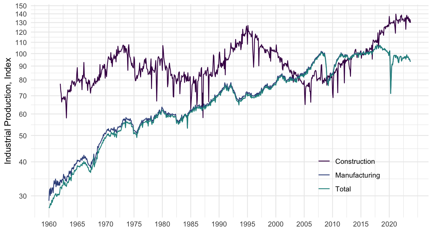

1990-

Code

DP_LIVE %>%
  filter(INDICATOR == "INDPROD", 
         LOCATION == "DEU", 
         FREQUENCY == "M") %>%
  left_join(DP_LIVE_var$SUBJECT, by = "SUBJECT") %>%
  month_to_date %>%
  filter(date >= as.Date("1990-01-01")) %>%
  ggplot + geom_line(aes(x = date, y = obsValue, color = Subject))+ 
  theme_minimal() + xlab("") + ylab("Industrial Production, Index") +
  scale_x_date(breaks = seq(1960, 2020, 5) %>% paste0("-01-01") %>% as.Date,
               labels = date_format("%Y")) +
  scale_y_log10(breaks = seq(-10, 200, 10),
                     labels = dollar_format(accuracy = 1, prefix = "")) +
  scale_color_manual(values = viridis(4)[1:3]) +
  theme(legend.position = c(0.8, 0.20),
        legend.title = element_blank())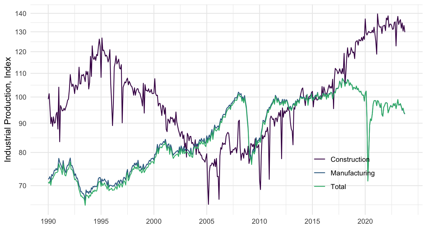

France

All

Code

DP_LIVE %>%
  filter(INDICATOR == "INDPROD", 
         LOCATION == "FRA", 
         FREQUENCY == "M") %>%
  left_join(DP_LIVE_var$SUBJECT %>%
              setNames(c("SUBJECT", "Subject")), by = "SUBJECT") %>%
  month_to_date %>%
  ggplot + geom_line(aes(x = date, y = obsValue, color = Subject))+ 
  theme_minimal() + xlab("") + ylab("Industrial Production, Index") +
  scale_x_date(breaks = seq(1960, 2020, 5) %>% paste0("-01-01") %>% as.Date,
               labels = date_format("%Y")) +
  scale_y_log10(breaks = seq(-10, 200, 10),
                     labels = dollar_format(accuracy = 1, prefix = "")) +
  scale_color_manual(values = viridis(4)[1:3]) +
  theme(legend.position = c(0.8, 0.20),
        legend.title = element_blank())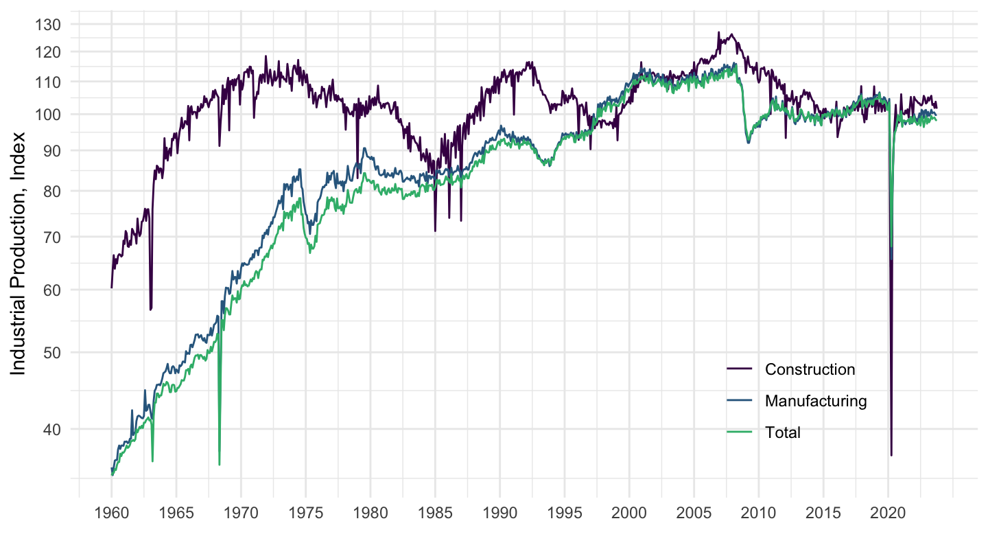

1990-

Code

DP_LIVE %>%
  filter(INDICATOR == "INDPROD", 
         LOCATION == "FRA", 
         FREQUENCY == "M") %>%
  left_join(DP_LIVE_var$SUBJECT %>%
              setNames(c("SUBJECT", "Subject")), by = "SUBJECT") %>%
  month_to_date %>%
  filter(date >= as.Date("1990-01-01")) %>%
  ggplot + geom_line(aes(x = date, y = obsValue, color = Subject))+ 
  theme_minimal() + xlab("") + ylab("Industrial Production, Index") +
  scale_x_date(breaks = seq(1960, 2020, 5) %>% paste0("-01-01") %>% as.Date,
               labels = date_format("%Y")) +
  scale_y_log10(breaks = seq(-10, 200, 10),
                     labels = dollar_format(accuracy = 1, prefix = "")) +
  scale_color_manual(values = viridis(4)[1:3]) +
  theme(legend.position = c(0.8, 0.20),
        legend.title = element_blank())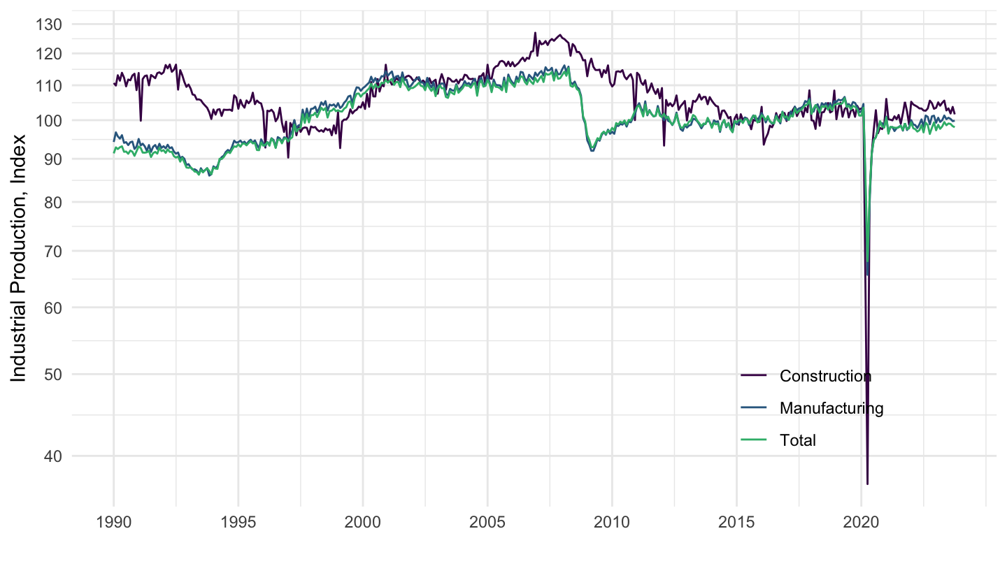

U.S.

Code

DP_LIVE %>%
  filter(INDICATOR == "INDPROD", 
         LOCATION == "USA", 
         FREQUENCY == "M") %>%
  left_join(DP_LIVE_var$SUBJECT %>%
              setNames(c("SUBJECT", "Subject")), by = "SUBJECT") %>%
  month_to_date %>%
  ggplot + geom_line(aes(x = date, y = obsValue, color = Subject))+ 
  theme_minimal() + xlab("") + ylab("Industrial Production, Index") +
  scale_x_date(breaks = seq(1960, 2020, 5) %>% paste0("-01-01") %>% as.Date,
               labels = date_format("%Y")) +
  scale_y_continuous(breaks = seq(-10, 200, 10),
                     labels = dollar_format(accuracy = 1, prefix = "")) +
  scale_color_manual(values = viridis(5)[1:4]) +
  theme(legend.position = c(0.8, 0.20),
        legend.title = element_blank())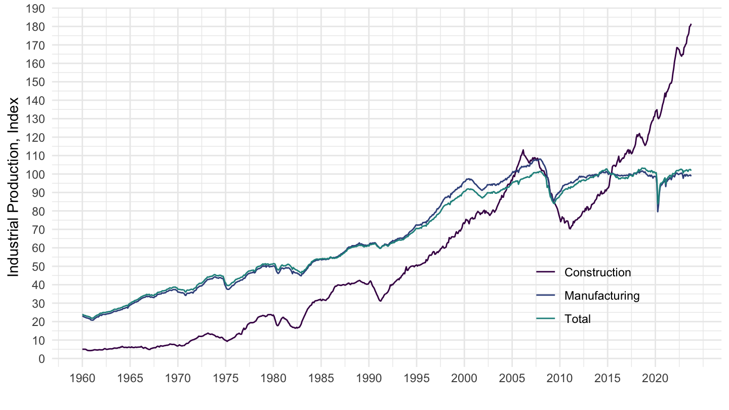

LT interest rates

All

Code

DP_LIVE %>%
  filter(INDICATOR == "LTINT", 
         LOCATION %in% c("USA", "FRA", "DEU"), 
         FREQUENCY == "M") %>%
  left_join(DP_LIVE_var$LOCATION %>%
              setNames(c("LOCATION", "Location")), by = "LOCATION") %>%
  month_to_date %>%
  ggplot + geom_line(aes(x = date, y = obsValue/100, color = Location)) + 
  geom_image(data = . %>%
               filter(date == as.Date("1982-01-01")) %>%
               mutate(date = as.Date("1982-01-01"),
                      image = paste0("../../icon/flag/", str_to_lower(gsub(" ", "-", Location)), ".png")),
             aes(x = date, y = obsValue/100, image = image), asp = 1.5) +
  theme_minimal() + xlab("") + ylab("Long-term interest rates") +
  scale_x_date(breaks = seq(1960, 2020, 5) %>% paste0("-01-01") %>% as.Date,
               labels = date_format("%Y")) +
  scale_y_continuous(breaks = 0.01*seq(-2, 30, 1),
                     labels = percent_format(accuracy = 1)) +
  scale_color_manual(values = c("#002395", "#000000", "#B22234")) +
  theme(legend.position = c(0.8, 0.80),
        legend.title = element_blank())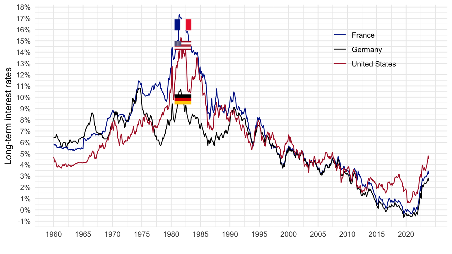

2000-

Code

DP_LIVE %>%
  filter(INDICATOR == "LTINT", 
         LOCATION %in% c("USA", "FRA", "DEU"), 
         FREQUENCY == "M") %>%
  left_join(DP_LIVE_var$LOCATION, by = "LOCATION") %>%
  month_to_date %>%
  filter(date >= as.Date("2000-01-01")) %>%
  ggplot + geom_line(aes(x = date, y = obsValue/100, color = Location))+ 
  geom_image(data = . %>%
               filter(date == as.Date("2018-07-01")) %>%
               mutate(date = as.Date("2018-07-01"),
                      image = paste0("../../icon/flag/", str_to_lower(gsub(" ", "-", Location)), ".png")),
             aes(x = date, y = obsValue/100, image = image), asp = 1.5) +
  theme_minimal() + xlab("") + ylab("Long-term interest rates") +
  scale_x_date(breaks = seq(1960, 2100, 2) %>% paste0("-01-01") %>% as.Date,
               labels = date_format("%Y")) +
  scale_y_continuous(breaks = 0.01*seq(-2, 30, 1),
                     labels = percent_format(accuracy = 1)) +
  scale_color_manual(values = c("#002395", "#000000", "#B22234")) +
  theme(legend.position = c(0.8, 0.80),
        legend.title = element_blank())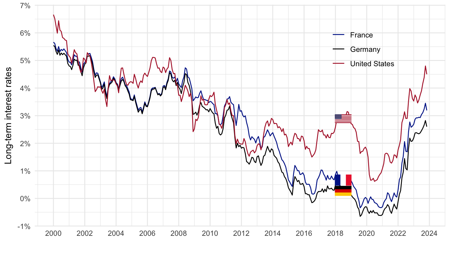

Part Time Employment Rate

Table

Code

DP_LIVE %>%
  filter(INDICATOR == "PARTEMP",
         SUBJECT == "TOT") %>%
  group_by(LOCATION) %>%
  summarise(Nobs = n())

# # A tibble: 52 × 2
#    LOCATION  Nobs
#    <chr>    <int>
#  1 AUS         24
#  2 AUT         30
#  3 BEL         42
#  4 BGR         25
#  5 BRA         23
#  6 CAN         49
#  7 CHE         29
#  8 CHL         29
#  9 COL         23
# 10 CRI         15
# # ℹ 42 more rows

Netherlands, Germany, Japan

Code

DP_LIVE %>%
  filter(LOCATION %in% c("DEU", "JPN", "NLD"), 
         INDICATOR == "PARTEMP", 
         SUBJECT == "TOT") %>%
  left_join(DP_LIVE_var$LOCATION, by = "LOCATION") %>%
  year_to_date() %>%
  mutate(obsValue = obsValue/100) %>%
  ggplot() + geom_line(aes(x = date, y = obsValue, color = Location)) +
  scale_color_manual(values = c("#000000", "#BC002D", "#21468B")) + add_3flags +
  theme_minimal() +
  scale_x_date(breaks = seq(1920, 2025, 2) %>% paste0("-01-01") %>% as.Date,
               labels = date_format("%Y")) +
  theme(legend.position = c(0.15, 0.8),
        legend.title = element_blank()) +
  scale_y_continuous(breaks = 0.01*seq(-6, 90, 2),
                     labels = percent_format(accuracy = 1)) +
  ylab("Part-time employment rate") + xlab("")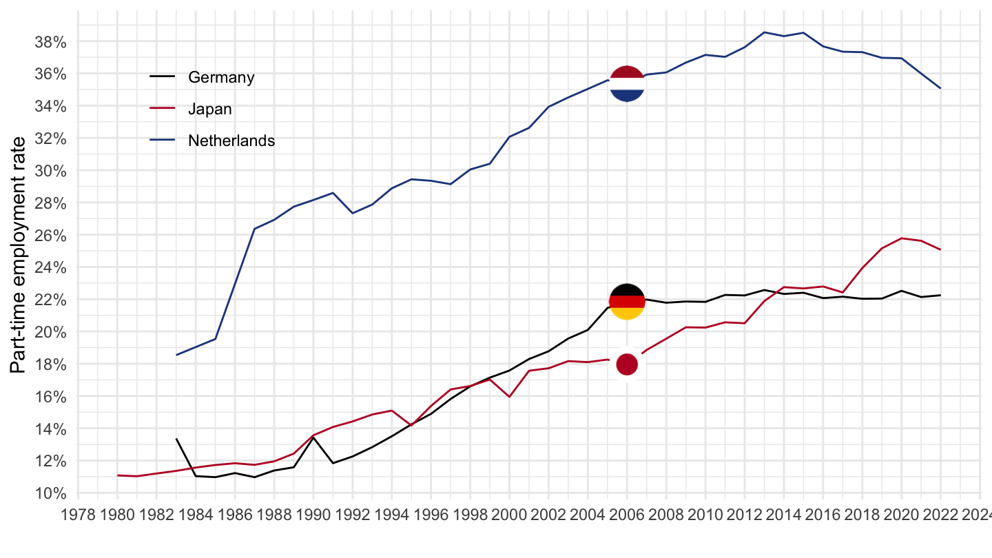

Netherlands, France, Germany, Japan

Code

DP_LIVE %>%
  filter(LOCATION %in% c("DEU", "FRA", "JPN", "NLD"), 
         INDICATOR == "PARTEMP", 
         SUBJECT == "TOT") %>%
  left_join(DP_LIVE_var$LOCATION, by = "LOCATION") %>%
  year_to_date() %>%
  mutate(obsValue = obsValue/100) %>%
  ggplot() + geom_line(aes(x = date, y = obsValue, color = Location)) +
  add_4flags +
  scale_color_manual(values = c("#002395", "#000000", "#BC002D", "#21468B")) +
  theme_minimal() +
  scale_x_date(breaks = seq(1920, 2025, 2) %>% paste0("-01-01") %>% as.Date,
               labels = date_format("%Y")) +
  theme(legend.position = c(0.15, 0.8),
        legend.title = element_blank()) +
  scale_y_continuous(breaks = 0.01*seq(-6, 90, 2),
                     labels = percent_format(accuracy = 1)) +
  ylab("Part-time employment rate") + xlab("")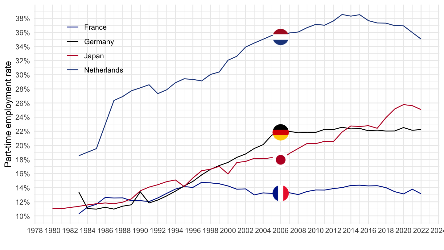

Germany, France

English

All

Code

DP_LIVE %>%
  filter(LOCATION %in% c("DEU", "FRA"), 
         INDICATOR == "PARTEMP", 
         SUBJECT == "TOT") %>%
  left_join(DP_LIVE_var$LOCATION, by = "LOCATION") %>%
  year_to_date() %>%
  mutate(obsValue = obsValue/100) %>%
  ggplot() + geom_line(aes(x = date, y = obsValue, color = Location)) +
  scale_color_manual(values = c("#002395", "#000000")) +
  geom_image(data = . %>%
               filter(date == as.Date("2006-01-01")) %>%
               mutate(image = paste0("../../icon/flag/round/", str_to_lower(gsub(" ", "-", Location)), ".png")),
             aes(x = date, y = obsValue, image = image), asp = 1.5) +
  theme_minimal() +
  scale_x_date(breaks = seq(1920, 2025, 2) %>% paste0("-01-01") %>% as.Date,
               labels = date_format("%Y")) +
  theme(legend.position = c(0.15, 0.8),
        legend.title = element_blank()) +
  scale_y_continuous(breaks = 0.01*seq(-6, 90, 2),
                     labels = percent_format(accuracy = 1)) +
  ylab("Part-time employment rate") + xlab("")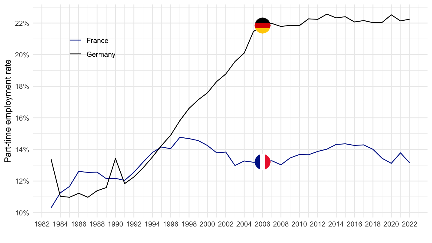

1995-

Code

DP_LIVE %>%
  filter(LOCATION %in% c("DEU", "FRA"), 
         INDICATOR == "PARTEMP", 
         SUBJECT == "TOT") %>%
  left_join(DP_LIVE_var$LOCATION, by = "LOCATION") %>%
  year_to_date() %>%
  mutate(obsValue = obsValue/100) %>%
  ggplot() + geom_line(aes(x = date, y = obsValue, color = Location)) +
  scale_color_manual(values = c("#002395", "#000000")) +
  geom_image(data = . %>%
               filter(date == as.Date("2006-01-01")) %>%
               mutate(image = paste0("../../icon/flag/round/", str_to_lower(gsub(" ", "-", Location)), ".png")),
             aes(x = date, y = obsValue, image = image), asp = 1.5) +
  theme_minimal() +
  scale_x_date(breaks = seq(1920, 2025, 2) %>% paste0("-01-01") %>% as.Date,
               labels = date_format("%Y")) +
  theme(legend.position = c(0.15, 0.8),
        legend.title = element_blank()) +
  scale_y_continuous(breaks = 0.01*seq(-6, 90, 2),
                     labels = percent_format(accuracy = 1)) +
  ylab("Taux d'emploi à temps partiel (%)") + xlab("")

French

Code

DP_LIVE %>%
  filter(LOCATION %in% c("DEU", "FRA"), 
         INDICATOR == "PARTEMP", 
         SUBJECT == "TOT") %>%
  left_join(DP_LIVE_var$LOCATION, by = "LOCATION") %>%
  year_to_date() %>%
  mutate(obsValue = obsValue/100) %>%
  ggplot() + geom_line(aes(x = date, y = obsValue, color = Location)) +
  scale_color_manual(values = c("#002395", "#000000")) +
  geom_image(data = . %>%
               filter(date == as.Date("2006-01-01")) %>%
               mutate(image = paste0("../../icon/flag/round/", str_to_lower(gsub(" ", "-", Location)), ".png")),
             aes(x = date, y = obsValue, image = image), asp = 1.5) +
  theme_minimal() +
  scale_x_date(breaks = seq(1920, 2025, 5) %>% paste0("-01-01") %>% as.Date,
               labels = date_format("%Y")) +
  theme(legend.position = "none") +
  scale_y_continuous(breaks = 0.01*seq(-6, 90, 2),
                     labels = percent_format(accuracy = 1),
                     limits = c(0, 0.24)) +
  ylab("Taux d'emploi à temps partiel") + xlab("")

French

Code

DP_LIVE %>%
  filter(LOCATION %in% c("DEU", "FRA"), 
         INDICATOR == "PARTEMP", 
         SUBJECT == "TOT") %>%
  left_join(DP_LIVE_var$LOCATION, by = "LOCATION") %>%
  year_to_date() %>%
  mutate(obsValue = obsValue/100) %>%
  ggplot() + geom_line(aes(x = date, y = obsValue, color = Location)) +
  scale_color_manual(values = c("#002395", "#000000")) +
  geom_image(data = . %>%
               filter(date == as.Date("2006-01-01")) %>%
               mutate(image = paste0("../../icon/flag/round/", str_to_lower(gsub(" ", "-", Location)), ".png")),
             aes(x = date, y = obsValue, image = image), asp = 1.5) +
  theme_minimal() +
  scale_x_date(breaks = seq(1920, 2025, 5) %>% paste0("-01-01") %>% as.Date,
               labels = date_format("%Y")) +
  theme(legend.position = "none") +
  scale_y_continuous(breaks = 0.01*seq(-6, 90, 2),
                     labels = percent_format(accuracy = 1),
                     limits = c(0, 0.24)) +
  ylab("Taux d'emploi à temps partiel") + xlab("")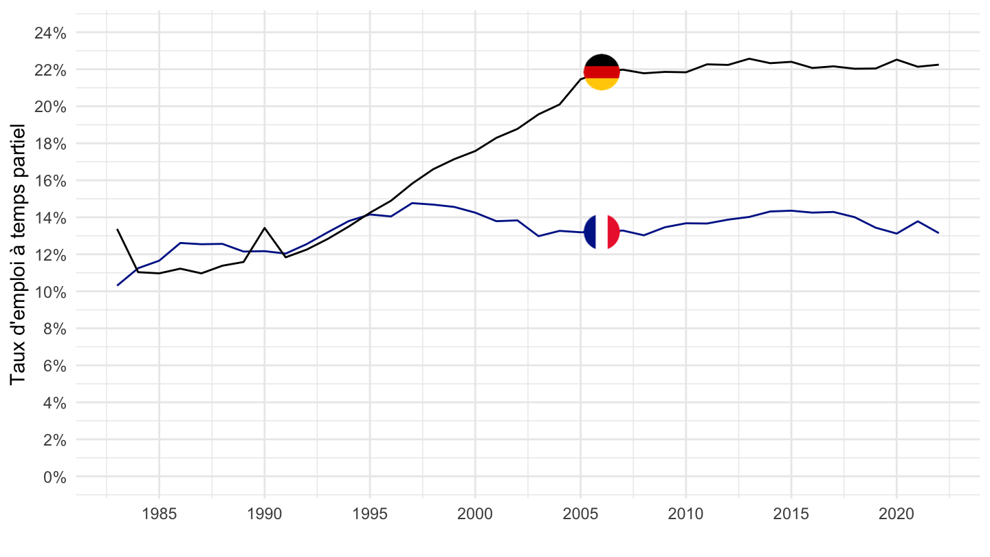

Tourism GDP

Code

DP_LIVE %>%
  filter(INDICATOR == "TOUR_GDP") %>%
  left_join(DP_LIVE_var$LOCATION, by = "LOCATION") %>%
  arrange(LOCATION, obsTime) %>%
  group_by(LOCATION, Location) %>%
  summarise(year = last(obsTime),
            `Tourism (% of GDP)` = round(last(obsValue), 1)) %>%
  arrange(-`Tourism (% of GDP)`) %>%
  mutate(`Tourism (% of GDP)` = paste0(`Tourism (% of GDP)`, "%")) %>%
  mutate(Flag = gsub(" ", "-", str_to_lower(gsub(" ", "-", Location))),
         Flag = paste0('<img src="../../icon/flag/vsmall/', Flag, '.png" alt="Flag">')) %>%
  select(Flag, everything()) %>%
  {if (is_html_output()) datatable(., filter = 'top', rownames = F, escape = F) else .}