Main Balance of Payments and International Investment Position items as share of GDP (BPM6)

Data - Eurostat

Author

Info

source	dataset	Title	.html	.rData
eurostat	bop_gdp6_q	Main Balance of Payments and International Investment Position items as share of GDP (BPM6)	2026-04-14	2026-04-14

Data on europe

source	dataset	Title	.html	.rData
eurostat	bop_gdp6_q	Main Balance of Payments and International Investment Position items as share of GDP (BPM6)	2026-04-14	2026-04-14
eurostat	nama_10_a10	Gross value added and income by A*10 industry breakdowns	2026-04-14	2026-04-14
eurostat	nama_10_a10_e	Employment by A*10 industry breakdowns	2026-04-09	2026-04-14
eurostat	nama_10_gdp	GDP and main components (output, expenditure and income)	2026-04-14	2026-04-14
eurostat	nama_10_lp_ulc	Labour productivity and unit labour costs	2026-04-14	2026-04-14
eurostat	namq_10_a10	Gross value added and income A*10 industry breakdowns	2026-04-14	2026-04-14
eurostat	namq_10_a10_e	Employment A*10 industry breakdowns	2025-05-24	2026-04-14
eurostat	namq_10_gdp	GDP and main components (output, expenditure and income)	2025-10-27	2026-04-14
eurostat	namq_10_lp_ulc	Labour productivity and unit labour costs	2026-03-24	2026-04-14
eurostat	namq_10_pc	Main GDP aggregates per capita	2026-03-24	2026-04-13
eurostat	nasa_10_nf_tr	Non-financial transactions	2026-04-14	2026-04-14
eurostat	nasq_10_nf_tr	NA	NA	NA
eurostat	tipsii40	Net international investment position - quarterly data, % of GDP	2026-04-15	2026-04-14

Data on macro

source	dataset	Title	.html	.rData
eurostat	nama_10_a10	Gross value added and income by A*10 industry breakdowns	2026-04-14	2026-04-14
eurostat	nama_10_a10_e	Employment by A*10 industry breakdowns	2026-04-09	2026-04-14
eurostat	nama_10_gdp	GDP and main components (output, expenditure and income)	2026-04-14	2026-04-14
eurostat	nama_10_lp_ulc	Labour productivity and unit labour costs	2026-04-14	2026-04-14
eurostat	namq_10_a10	Gross value added and income A*10 industry breakdowns	2026-04-14	2026-04-14
eurostat	namq_10_a10_e	Employment A*10 industry breakdowns	2025-05-24	2026-04-14
eurostat	namq_10_gdp	GDP and main components (output, expenditure and income)	2025-10-27	2026-04-14
eurostat	namq_10_lp_ulc	Labour productivity and unit labour costs	2026-03-24	2026-04-14
eurostat	namq_10_pc	Main GDP aggregates per capita	2026-03-24	2026-04-13
eurostat	nasa_10_nf_tr	Non-financial transactions	2026-04-14	2026-04-14
eurostat	nasq_10_nf_tr	NA	NA	NA
fred	gdp	Gross Domestic Product	2026-04-14	2026-04-12
oecd	QNA	Quarterly National Accounts	2026-04-15	2026-04-14
oecd	SNA_TABLE1	Gross domestic product (GDP)	2026-04-15	2025-05-24
oecd	SNA_TABLE14A	Non-financial accounts by sectors	2026-04-15	2024-06-30
oecd	SNA_TABLE2	Disposable income and net lending - net borrowing	2024-07-01	2024-04-11
oecd	SNA_TABLE6A	Value added and its components by activity, ISIC rev4	2024-07-01	2024-06-30
wdi	NE.RSB.GNFS.ZS	External balance on goods and services (% of GDP)	2026-04-14	2026-04-14
wdi	NY.GDP.MKTP.CD	NA	NA	NA
wdi	NY.GDP.MKTP.PP.CD	GDP, PPP (current international D)	2026-04-14	2026-04-14
wdi	NY.GDP.PCAP.CD	GDP per capita (current USD)	2026-04-14	2026-04-14
wdi	NY.GDP.PCAP.KD	GDP per capita (constant 2015 USD)	2026-04-14	2026-04-14
wdi	NY.GDP.PCAP.PP.CD	GDP per capita, PPP (current international D)	2026-02-23	2026-04-14
wdi	NY.GDP.PCAP.PP.KD	GDP per capita, PPP (constant 2011 international D)	2026-04-14	2026-04-14

LAST_COMPILE

LAST_COMPILE
2026-04-16

Last

Code

bop_gdp6_q %>%
  group_by(time) %>%
  summarise(Nobs = n()) %>%
  arrange(desc(time)) %>%
  head(1) %>%
  print_table_conditional()

time	Nobs
2025Q4	3713

unit

Code

bop_gdp6_q %>%
  left_join(unit, by = "unit") %>%
  group_by(unit, Unit) %>%
  summarise(Nobs = n()) %>%
  arrange(-Nobs) %>%
  print_table_conditional()

unit	Unit	Nobs
PC_GDP	Percentage of gross domestic product (GDP)	555422
PC_GDP_3Y	Percentage of GDP - three-year average	41007

s_adj

Code

bop_gdp6_q %>%
  left_join(s_adj, by = "s_adj") %>%
  group_by(s_adj, S_adj) %>%
  summarise(Nobs = n()) %>%
  arrange(-Nobs) %>%
  print_table_conditional()

s_adj	S_adj	Nobs
NSA	Unadjusted data (i.e. neither seasonally adjusted nor calendar adjusted data)	586568
SCA	Seasonally and calendar adjusted data	9861

bop_item

Code

bop_gdp6_q %>%
  left_join(bop_item, by = "bop_item") %>%
  group_by(bop_item, Bop_item) %>%
  summarise(Nobs = n()) %>%
  arrange(-Nobs) %>%
  print_table_conditional()

bop_item	Bop_item	Nobs
S	Services	90819
G	Goods	89831
GS	Goods and services	87311
FA__D__F	Financial account; direct investment	64972
IN2	Secondary income	52118
KA	Capital account	51590
FA__P__F	Financial account; portfolio investment	34035
FA	Financial account	32893
CA	Current account	23519
IN1	Primary income	22920
CKA	Current plus capital account (balance = net lending (+) / net borrowing (-))	22443
S_X_CG	Services excluding transport and financial services	15166
FA__FNED	Net external debt	4736
FA__NENDI	Net international investment position excluding non-defaultable instruments	3806
FA__TXR__F	Financial account excluding reserve assets	270

stk_flow

Code

bop_gdp6_q %>%
  left_join(stk_flow, by = "stk_flow") %>%
  group_by(stk_flow, Stk_flow) %>%
  summarise(Nobs = n()) %>%
  arrange(-Nobs) %>%
  print_table_conditional()

stk_flow	Stk_flow	Nobs
CRE	Credit	119661
DEB	Debit	108052
BAL	Balance	107788
CRE_DEB_SUM	Sum of credits and debits	66085
CRE_DEB_AVG	Average of credits and debits	54262
ASS	Assets	32484
NET	Net	27873
LIAB	Liabilities	27454
N_LE	Net positions at the end of period	18903
A_LE	Assets - positions at the end of period	15353
L_LE	Liabilities - positions at the end of period	14621
NE_LE	Net liabilities (liabilities minus assets)	3893

partner

Code

bop_gdp6_q %>%
  left_join(partner, by = "partner") %>%
  group_by(partner, Partner) %>%
  summarise(Nobs = n()) %>%
  arrange(-Nobs) %>%
  mutate(Partner = ifelse(partner == "DE", "Germany", Partner)) %>%
  mutate(Flag = gsub(" ", "-", str_to_lower(Partner)),
         Flag = paste0('<img src="../../bib/flags/vsmall/', Flag, '.png" alt="Flag">')) %>%
  select(Flag, everything()) %>%
  {if (is_html_output()) datatable(., filter = 'top', rownames = F, escape = F) else .}

geo

Code

bop_gdp6_q %>%
  left_join(geo, by = "geo") %>%
  group_by(geo, Geo) %>%
  summarise(Nobs = n()) %>%
  arrange(-Nobs) %>%
  {if (is_html_output()) datatable(., filter = 'top', rownames = F) else .}

time

Code

bop_gdp6_q %>%
  group_by(time) %>%
  summarise(Nobs = n()) %>%
  arrange(desc(time)) %>%
  {if (is_html_output()) datatable(., filter = 'top', rownames = F) else .}

France, Germany, Italy

Last

Code

bop_gdp6_q %>%
  filter(freq == "Q") %>%
  quarter_to_date %>%
  filter(geo %in% c("FR", "DE", "IT"),
         date == max(date, na.rm = T),
         !(stk_flow %in% c("CRE", "DEB"))) %>%
  left_join(geo, by = "geo") %>%
  left_join(bop_item, by = "bop_item") %>%
  left_join(stk_flow, by = "stk_flow") %>%
  select(-geo) %>%
  spread(Geo, values) %>%
  select_if(~ n_distinct(.) > 1) %>%
  {if (is_html_output()) datatable(., filter = 'top', rownames = F) else .}

Germany, Spain, France, Italy, Netherlands, Europe

Current account Balance

All

Code

bop_gdp6_q %>%
  filter(freq == "Q") %>%
  filter(((geo %in% c("DE", "ES", "FR", "IT", "NL", "EA20")) & partner == "WRL_REST") |
           (geo == "EA20" & partner == "EXT_EA20"),
         unit == "PC_GDP",
         bop_item == "CA",
         s_adj == "NSA",
         stk_flow == "BAL") %>%
  left_join(geo, by = "geo") %>%
  left_join(stk_flow, by = "stk_flow") %>%
  select_if(~ n_distinct(.) > 1) %>%
  quarter_to_date %>%
  mutate(Geo = ifelse(geo == "EA20", "Europe", Geo)) %>%
  left_join(colors, by = c("Geo" = "country")) %>%
  mutate(values = values/100) %>%
  ggplot + geom_line(aes(x = date, y = values, color = color)) + theme_minimal() +
  scale_color_identity() + add_6flags +
  scale_x_date(breaks = as.Date(paste0(seq(1960, 2100, 2), "-01-01")),
               labels = date_format("%Y")) +
  xlab("") + ylab("Current account balance") +
  scale_y_continuous(breaks = 0.01*seq(-100, 200, 2),
                     labels = scales::percent_format(accuracy = 1))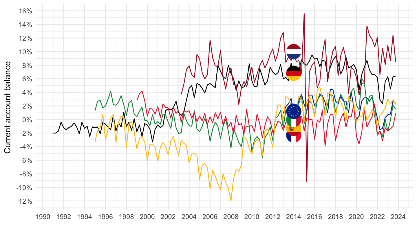

2006-

Code

bop_gdp6_q %>%
  filter(freq == "Q") %>%
  filter(((geo %in% c("DE", "ES", "FR", "IT", "NL", "EA20")) & partner == "WRL_REST") |
           (geo == "EA20" & partner == "EXT_EA20"),
         unit == "PC_GDP",
         bop_item == "CA",
         s_adj == "NSA",
         stk_flow == "BAL") %>%
  left_join(geo, by = "geo") %>%
  left_join(stk_flow, by = "stk_flow") %>%
  select_if(~ n_distinct(.) > 1) %>%
  quarter_to_date %>%
  filter(date >=as.Date("2006-01-01")) %>%
  mutate(Geo = ifelse(geo == "EA20", "Europe", Geo)) %>%
  left_join(colors, by = c("Geo" = "country")) %>%
  mutate(values = values/100) %>%
  ggplot + geom_line(aes(x = date, y = values, color = color)) + theme_minimal() +
  scale_color_identity() + add_6flags +
  scale_x_date(breaks = as.Date(paste0(seq(1960, 2100, 2), "-01-01")),
               labels = date_format("%Y")) +
  xlab("") + ylab("Current account balance") +
  scale_y_continuous(breaks = 0.01*seq(-100, 200, 2),
                     labels = scales::percent_format(accuracy = 1))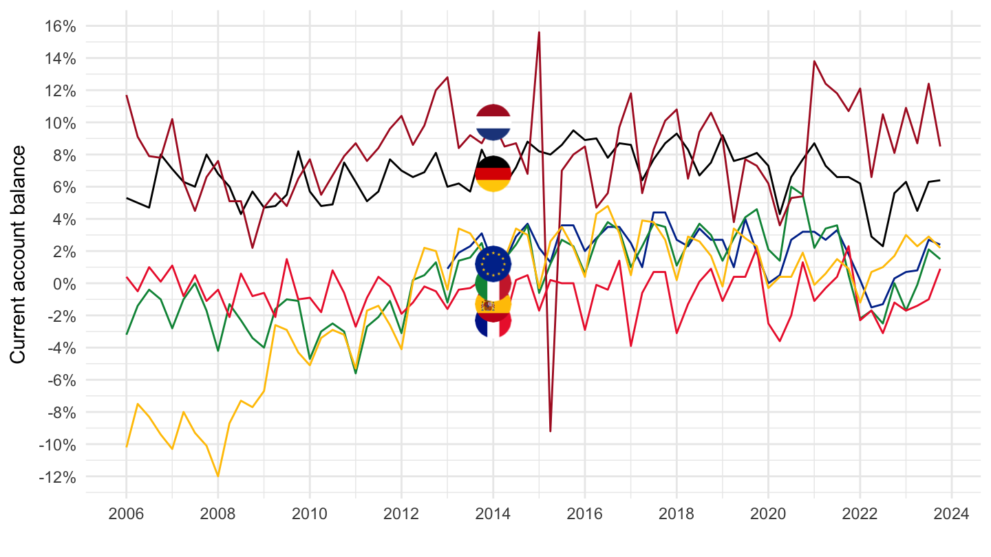

2012-

Code

bop_gdp6_q %>%
  filter(freq == "Q") %>%
  filter(((geo %in% c("DE", "ES", "FR", "IT", "NL", "EA20")) & partner == "WRL_REST") |
           (geo == "EA20" & partner == "EXT_EA20"),
         unit == "PC_GDP",
         bop_item == "CA",
         s_adj == "NSA",
         stk_flow == "BAL") %>%
  left_join(geo, by = "geo") %>%
  left_join(stk_flow, by = "stk_flow") %>%
  select_if(~ n_distinct(.) > 1) %>%
  quarter_to_date %>%
  filter(date >=as.Date("2012-01-01")) %>%
  mutate(Geo = ifelse(geo == "EA20", "Europe", Geo)) %>%
  left_join(colors, by = c("Geo" = "country")) %>%
  mutate(values = values/100) %>%
  ggplot + geom_line(aes(x = date, y = values, color = color)) + theme_minimal() +
  scale_color_identity() + add_6flags +
  scale_x_date(breaks = as.Date(paste0(seq(1960, 2100, 1), "-01-01")),
               labels = date_format("%Y")) +
  xlab("") + ylab("Current account balance") +
  scale_y_continuous(breaks = 0.01*seq(-100, 200, 2),
                     labels = scales::percent_format(accuracy = 1))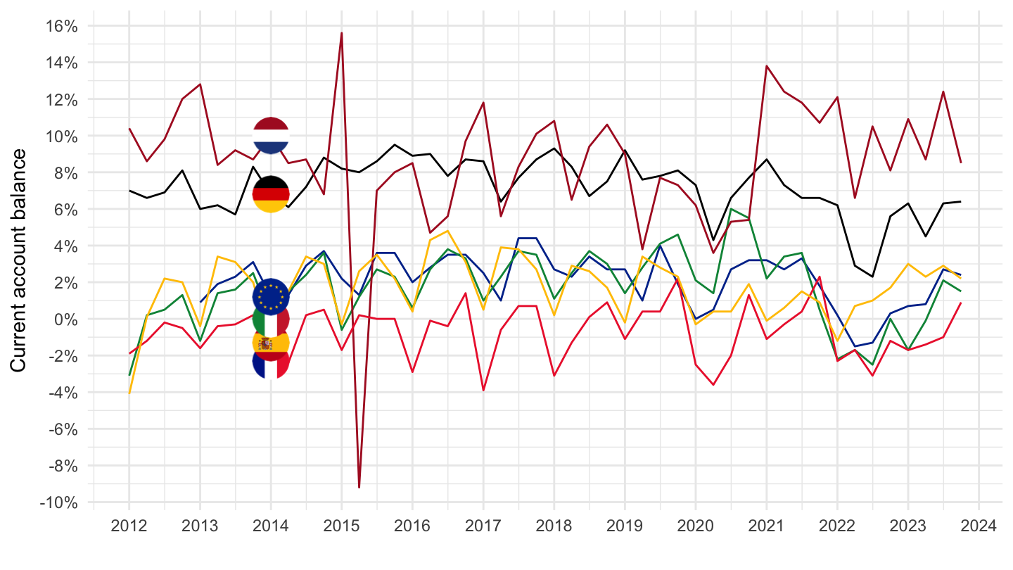

Net Investment Positions (FA__NENDI)

Code

bop_gdp6_q %>%
  filter(freq == "Q") %>%
  filter(((geo %in% c("DE", "ES", "FR", "IT", "NL", "EA20")) & partner == "WRL_REST") |
           (geo == "EA20" & partner == "EXT_EA20"),
         unit == "PC_GDP",
         bop_item == "FA__NENDI",
         s_adj == "NSA") %>%
  left_join(geo, by = "geo") %>%
  left_join(stk_flow, by = "stk_flow") %>%
  select_if(~ n_distinct(.) > 1) %>%
  quarter_to_date %>%
  mutate(Geo = ifelse(geo == "EA20", "Europe", Geo)) %>%
  left_join(colors, by = c("Geo" = "country")) %>%
  mutate(values = values/100) %>%
  ggplot + geom_line(aes(x = date, y = values, color = color)) + theme_minimal() +
  scale_color_identity() + add_5flags +
  scale_x_date(breaks = as.Date(paste0(seq(1960, 2100, 5), "-01-01")),
               labels = date_format("%Y")) +
  xlab("") + ylab("Net international investment positions (% of GDP)") +
  scale_y_continuous(breaks = 0.01*seq(-100, 200, 10),
                     labels = scales::percent_format(accuracy = 1))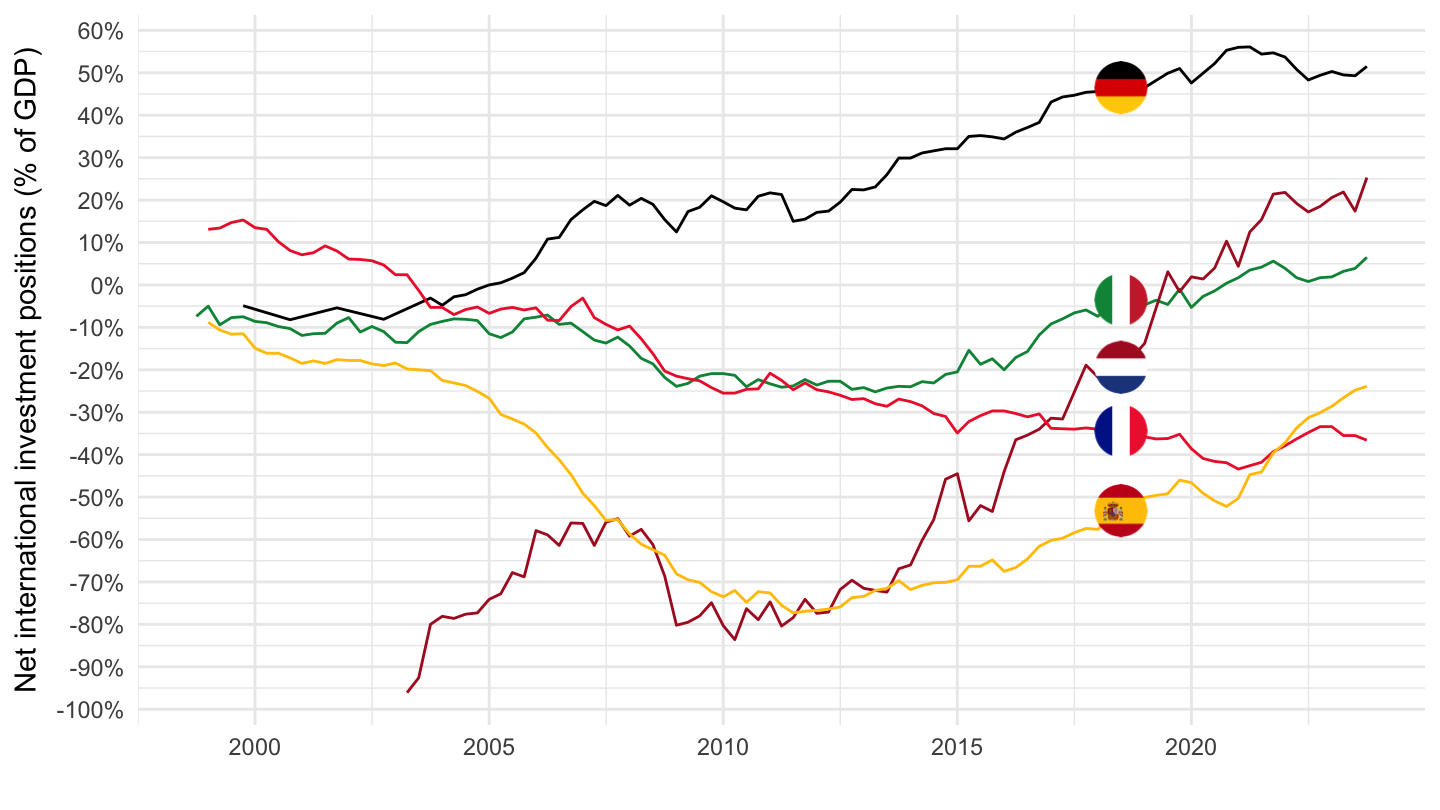

Goods and Services

Code

bop_gdp6_q %>%
  filter(freq == "Q") %>%
  filter(((geo %in% c("DE", "ES", "FR", "IT", "NL", "EA20")) & partner == "WRL_REST") |
           (geo == "EA20" & partner == "EXT_EA20"),
         unit == "PC_GDP",
         bop_item == "GS",
         s_adj == "NSA",
         stk_flow == "BAL") %>%
  left_join(geo, by = "geo") %>%
  left_join(stk_flow, by = "stk_flow") %>%
  select_if(~ n_distinct(.) > 1) %>%
  quarter_to_date %>%
  mutate(Geo = ifelse(geo == "EA20", "Europe", Geo)) %>%
  left_join(colors, by = c("Geo" = "country")) %>%
  mutate(values = values/100) %>%
  ggplot + geom_line(aes(x = date, y = values, color = color)) + theme_minimal() +
  scale_color_identity() + add_6flags +
  scale_x_date(breaks = as.Date(paste0(seq(1960, 2100, 5), "-01-01")),
               labels = date_format("%Y")) +
  xlab("") + ylab("Goods and Services") +
  scale_y_continuous(breaks = 0.01*seq(-100, 200, 2),
                     labels = scales::percent_format(accuracy = 1))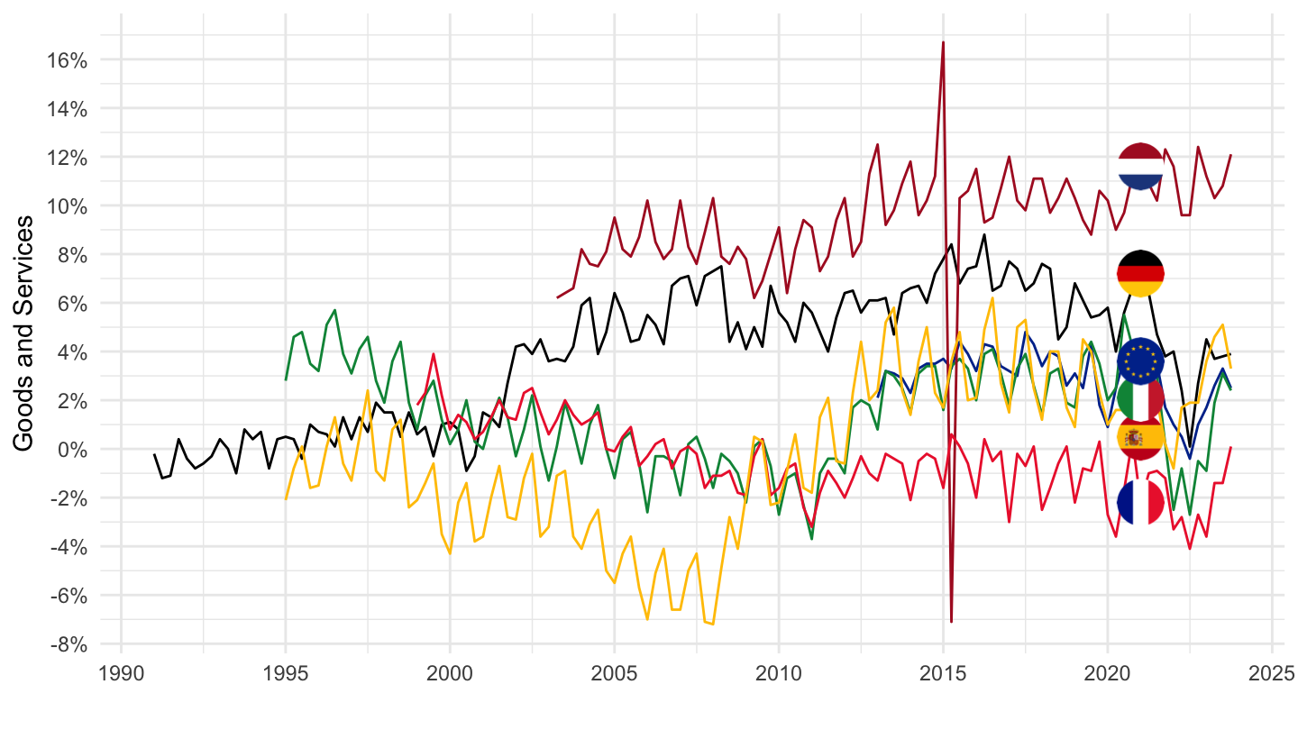

Goods

Code

bop_gdp6_q %>%
  filter(freq == "Q") %>%
  filter(((geo %in% c("DE", "ES", "FR", "IT", "NL", "EA20")) & partner == "WRL_REST") |
           (geo == "EA20" & partner == "EXT_EA20"),
         unit == "PC_GDP",
         bop_item == "G",
         s_adj == "NSA",
         stk_flow == "BAL") %>%
  left_join(geo, by = "geo") %>%
  left_join(stk_flow, by = "stk_flow") %>%
  select_if(~ n_distinct(.) > 1) %>%
  quarter_to_date %>%
  mutate(Geo = ifelse(geo == "EA20", "Europe", Geo)) %>%
  left_join(colors, by = c("Geo" = "country")) %>%
  mutate(values = values/100) %>%
  ggplot + geom_line(aes(x = date, y = values, color = color)) + theme_minimal() +
  scale_color_identity() + add_6flags +
  scale_x_date(breaks = as.Date(paste0(seq(1960, 2100, 5), "-01-01")),
               labels = date_format("%Y")) +
  xlab("") + ylab("Goods") +
  scale_y_continuous(breaks = 0.01*seq(-100, 200, 2),
                     labels = scales::percent_format(accuracy = 1))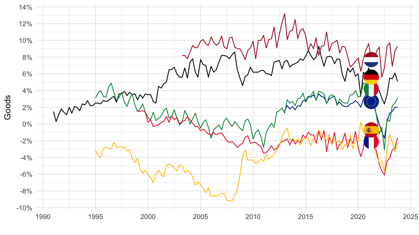

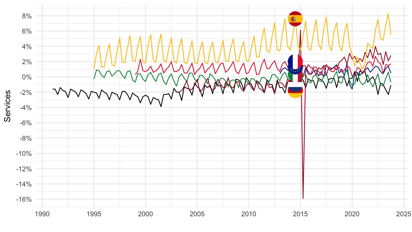
Services

Code

bop_gdp6_q %>%
  filter(freq == "Q") %>%
  filter(((geo %in% c("DE", "ES", "FR", "IT", "NL", "EA20")) & partner == "WRL_REST") |
           (geo == "EA20" & partner == "EXT_EA20"),
         unit == "PC_GDP",
         bop_item == "S",
         s_adj == "NSA",
         stk_flow == "BAL") %>%
  left_join(geo, by = "geo") %>%
  left_join(stk_flow, by = "stk_flow") %>%
  select_if(~ n_distinct(.) > 1) %>%
  quarter_to_date %>%
  mutate(Geo = ifelse(geo == "EA20", "Europe", Geo)) %>%
  left_join(colors, by = c("Geo" = "country")) %>%
  mutate(values = values/100) %>%
  ggplot + geom_line(aes(x = date, y = values, color = color)) + theme_minimal() +
  scale_color_identity() + add_6flags +
  scale_x_date(breaks = as.Date(paste0(seq(1960, 2100, 5), "-01-01")),
               labels = date_format("%Y")) +
  xlab("") + ylab("Services") +
  scale_y_continuous(breaks = 0.01*seq(-100, 200, 2),
                     labels = scales::percent_format(accuracy = 1))