Risk Assessment Indicators
Data - ECB
Info
- Data Structure Definition. (DSD) html
Data on monetary policy
| source | dataset | Title | .html | .rData |
|---|---|---|---|---|
| bdf | FM | Marché financier, taux | 2026-07-22 | 2026-07-22 |
| bdf | MIR | Taux d'intérêt - Zone euro | 2026-07-22 | 2026-07-22 |
| bdf | MIR1 | Taux d'intérêt - France | 2026-07-23 | 2026-07-23 |
| bis | CBPOL | Policy Rates, Daily | 2026-07-18 | 2026-07-22 |
| ecb | BSI | Balance Sheet Items | 2026-07-23 | 2026-07-22 |
| ecb | BSI_PUB | Balance Sheet Items - Published series | 2026-07-23 | 2026-07-22 |
| ecb | FM | Financial market data | 2026-07-23 | 2026-07-22 |
| ecb | ILM | Internal Liquidity Management | 2026-07-23 | 2026-07-22 |
| ecb | ILM_PUB | Internal Liquidity Management - Published series | 2026-07-23 | 2026-07-22 |
| ecb | MIR | MFI Interest Rate Statistics | 2026-07-23 | 2026-07-22 |
| ecb | RAI | Risk Assessment Indicators | 2026-07-23 | 2026-07-23 |
| ecb | SUP | Supervisory Banking Statistics | 2026-07-23 | 2026-07-23 |
| ecb | YC | Financial market data - yield curve | 2026-07-23 | 2026-07-23 |
| ecb | YC_PUB | Financial market data - yield curve - Published series | 2026-07-23 | 2026-07-23 |
| ecb | liq_daily | Daily Liquidity | 2026-07-23 | 2026-07-23 |
| eurostat | ei_mfir_m | Interest rates - monthly data | 2026-07-23 | 2026-07-23 |
| eurostat | irt_st_m | Money market interest rates - monthly data | 2026-07-23 | 2026-07-23 |
| fred | r | Interest Rates | 2026-07-22 | 2026-07-22 |
| oecd | MEI | Main Economic Indicators | 2024-04-16 | 2025-07-24 |
| oecd | MEI_FIN | Monthly Monetary and Financial Statistics (MEI) | 2024-09-15 | 2025-07-24 |
Data on interest rates
| source | dataset | Title | .html | .rData |
|---|---|---|---|---|
| bdf | FM | Marché financier, taux | 2026-07-22 | 2026-07-22 |
| bdf | MIR | Taux d'intérêt - Zone euro | 2026-07-22 | 2026-07-22 |
| bdf | MIR1 | Taux d'intérêt - France | 2026-07-23 | 2026-07-23 |
| bis | CBPOL_D | Policy Rates, Daily | 2026-07-18 | 2025-08-20 |
| bis | CBPOL_M | Policy Rates, Monthly | 2026-07-22 | 2024-04-19 |
| ecb | FM | Financial market data | 2026-07-23 | 2026-07-22 |
| ecb | MIR | MFI Interest Rate Statistics | 2026-07-23 | 2026-07-22 |
| eurostat | ei_mfir_m | Interest rates - monthly data | 2026-07-23 | 2026-07-23 |
| eurostat | irt_lt_mcby_d | EMU convergence criterion series - daily data | 2026-07-23 | 2025-07-24 |
| eurostat | irt_st_m | Money market interest rates - monthly data | 2026-07-23 | 2026-07-23 |
| fred | r | Interest Rates | 2026-07-22 | 2026-07-22 |
| oecd | MEI | Main Economic Indicators | 2024-04-16 | 2025-07-24 |
| oecd | MEI_FIN | Monthly Monetary and Financial Statistics (MEI) | 2024-09-15 | 2025-07-24 |
| wdi | FR.INR.DPST | Deposit interest rate (%) | 2022-09-27 | 2026-07-22 |
| wdi | FR.INR.LEND | Lending interest rate (%) | 2026-07-22 | 2026-07-22 |
| wdi | FR.INR.RINR | Real interest rate (%) | 2026-01-11 | 2026-07-22 |
LAST_COMPILE
| LAST_COMPILE |
|---|
| 2026-07-24 |
Last
| TIME_PERIOD | FREQ | Nobs |
|---|---|---|
| 2026-Q1 | Q | 158 |
| 2026-05 | M | 373 |
DD_ECON_CONCEPT
Code
RAI %>%
  left_join(DD_ECON_CONCEPT, by = "DD_ECON_CONCEPT") %>%
  group_by(DD_ECON_CONCEPT, Dd_econ_concept) %>%
  summarise(Nobs = n()) %>%
  arrange(-Nobs) %>%
print_table_conditional()| DD_ECON_CONCEPT | Dd_econ_concept | Nobs |
|---|---|---|
| LMGBLNFCH | Lending margin on new business loans to non-financial corporations and households | 8436 |
| LMGOLNFCH | Lending margin on outstanding loans to non-financial corporations and households | 8413 |
| IBL1TL | Share of interbank loans in total loans | 8397 |
| CT1DGGV | Share of other MFIs credit to domestic general government in total assets, excluding remaining assets | 8036 |
| LC1DHHS | Share of other MFIs loans to domestic households for house purchase in total credit to other domestic residents | 7959 |
| LEVR | Leverage ratio | 7882 |
| NDEPFUN | Non-deposit funding | 7786 |
| SVLHHNFC | Share of new loans with a floating rate or an initial rate fixation period of up to one year in total new loans from MFIs to households and non-financial corporations | 7693 |
| SVLHPHH | Share of new loans to households for house purchase with a floating rate or an initial rate fixation period of up to one year in total new loans from MFIs to households | 7693 |
| LMGLHH | MFIs lending margins on loans for house purchase | 7138 |
| LMGLNFC | MFIs lending margins on loans to non-financial corporations (NFC) | 7138 |
| GRNLHHNFC | Annual growth rate of MFIs new loans to households and non-financial corporations | 6783 |
| ST1TMF | Share of short-term funding in total market funding | 6676 |
| MMTCH | Maturity mismatch | 5877 |
| FXL1TL | Share of other MFI FX loans in total loans (excluding inter-MFI loans) | 2807 |
| LTD | Loans to deposits ratio | 2745 |
| LA1STL | Share of liquid assets in short term liabilities | 2177 |
| OTHOFI1 | Total assets of other financial institutions (OFIs) excluding financial vehicle corporations (FVCs), outstanding amounts at the end of the period (stocks) | 1943 |
| OTHOFI4 | Total assets of other financial institutions (OFIs) excluding financial vehicle corporations (FVCs), financial transactions (flows) | 1941 |
| SVLOAHH | NA | 1750 |
| SVLOANFC | NA | 1750 |
| IFOFI1 | Total assets of MMF and non-MMF investment funds and other financial institutions (OFIs), outstanding amounts at the end of the period (stocks) | 285 |
| IFOFI4 | Total assets of MMF and non-MMF investment funds and other financial institutions (OFIs), financial transactions (flows) | 285 |
| CRED1 | Credit institutions (MFIs excluding the ESCB and MMFs), outstanding amounts at the end of the period (stocks) | 194 |
| CREDA | Growth rate of total assets of credit institutions (MFIs excluding the ESCB and MMFs) | 186 |
| ICPFA | Growth rate of total assets of insurance corporations and pension funds | 186 |
| IFOFIA | Growth rate of total assets of MMF and non-MMF investment funds and other financial institutions (OFIs) | 182 |
DD_SUFFIX
Code
RAI %>%
  left_join(DD_SUFFIX, by = "DD_SUFFIX") %>%
  group_by(DD_SUFFIX, Dd_suffix) %>%
  summarise(Nobs = n()) %>%
  arrange(-Nobs) %>%
print_table_conditional()| DD_SUFFIX | Dd_suffix | Nobs |
|---|---|---|
| Z | Not applicable | 114883 |
| E | Euro | 4648 |
| P10 | Currency ratio on total currency | 2807 |
SOURCE_DATA
Code
RAI %>%
  left_join(SOURCE_DATA, by = "SOURCE_DATA") %>%
  group_by(SOURCE_DATA, Source_data) %>%
  summarise(Nobs = n()) %>%
  arrange(-Nobs) %>%
print_table_conditional()| SOURCE_DATA | Source_data | Nobs |
|---|---|---|
| BSI | Based on BSI data | 64222 |
| MIR | Based on MIR data | 53294 |
| QSA | Based on quarterly sector accounts data | 4636 |
| ICPF | Based on ICPF data | 186 |
DD_SUFFIX
Code
RAI %>%
  left_join(DD_SUFFIX, by = "DD_SUFFIX") %>%
  group_by(DD_SUFFIX, Dd_suffix) %>%
  summarise(Nobs = n()) %>%
  arrange(-Nobs) %>%
print_table_conditional()| DD_SUFFIX | Dd_suffix | Nobs |
|---|---|---|
| Z | Not applicable | 114883 |
| E | Euro | 4648 |
| P10 | Currency ratio on total currency | 2807 |
FREQ
Code
RAI %>%
  left_join(FREQ, by = "FREQ") %>%
  group_by(FREQ, Freq) %>%
  summarise(Nobs = n()) %>%
  arrange(-Nobs) %>%
print_table_conditional()| FREQ | Freq | Nobs |
|---|---|---|
| M | Monthly | 105907 |
| Q | Quarterly | 16431 |
REF_AREA
Code
RAI %>%
  left_join(REF_AREA, by = "REF_AREA") %>%
  group_by(REF_AREA, Ref_area) %>%
  summarise(Nobs = n()) %>%
  arrange(-Nobs) %>%
  mutate(Flag = gsub(" ", "-", str_to_lower(gsub(" ", "-", Ref_area))),
         Flag = paste0('<img src="../../icon/flag/vsmall/', Flag, '.png" alt="Flag">')) %>%
  select(Flag, everything()) %>%
  {if (is_html_output()) datatable(., filter = 'top', rownames = F, escape = F) else .}
Table: Average 2016-2022
Code
RAI %>%
  filter(FREQ == "M") %>%
  left_join(REF_AREA, by = "REF_AREA") %>%
  left_join(DD_ECON_CONCEPT, by = "DD_ECON_CONCEPT") %>%
  month_to_date %>%
  filter(date >= as.Date("2016-01-01")) %>%
  group_by(DD_ECON_CONCEPT, Dd_econ_concept, REF_AREA, Ref_area) %>%
  summarise(OBS_VALUE = mean(OBS_VALUE),
            Nobs = n()) %>%
  print_table_conditional()
France
Table
Code
RAI %>%
  filter(FREQ == "M",
         REF_AREA %in% c("FR", "U2")) %>%
  select_if(~ n_distinct(.) > 1) %>%
  left_join(REF_AREA, by = "REF_AREA") %>%
  group_by(DD_ECON_CONCEPT, Ref_area) %>%
  filter(TIME_PERIOD == max(TIME_PERIOD)) %>%
  left_join(DD_ECON_CONCEPT, by = "DD_ECON_CONCEPT") %>%
  select(Ref_area, DD_ECON_CONCEPT, OBS_VALUE) %>%
  spread(Ref_area, OBS_VALUE) %>%
  arrange(-`France`) %>%
print_table_conditional()| DD_ECON_CONCEPT | Euro area (Member States and Institutions of the Euro Area) changing composition | France |
|---|---|---|
| MMTCH | 77.310265 | 78.5163575 |
| ST1TMF | 68.877095 | 77.1582087 |
| SVLHHNFC | 64.396321 | 38.4837738 |
| IBL1TL | 24.592109 | 36.9828106 |
| LC1DHHS | NA | 36.1629339 |
| NDEPFUN | 14.591115 | 15.6445765 |
| LEVR | 8.313538 | 7.2250397 |
| GRNLHHNFC | NA | 6.4463453 |
| CT1DGGV | NA | 4.4549032 |
| SVLHPHH | 15.455676 | 3.2691609 |
| LMGLNFC | NA | 1.2730756 |
| LMGBLNFCH | NA | 1.1336748 |
| LMGLHH | NA | 0.8359050 |
| LMGOLNFCH | NA | 0.2646171 |
SVLHHNFC, LC1DHHS
Code
RAI %>%
  filter(DD_ECON_CONCEPT %in% c("SVLHHNFC", "LC1DHHS"),
         REF_AREA %in% c("FR", "U2")) %>%
  left_join(REF_AREA, by = "REF_AREA") %>%
  left_join(DD_ECON_CONCEPT, by = "DD_ECON_CONCEPT") %>%
  month_to_date %>%
  select_if(~n_distinct(.) > 1) %>%
  mutate(Ref_area = ifelse(REF_AREA == "U2", "Europe", Ref_area)) %>%
  left_join(colors, by = c("Ref_area" = "country")) %>%
  mutate(OBS_VALUE = OBS_VALUE/100) %>%
  ggplot(.) + theme_minimal() + xlab("") + ylab("Share of variable rate") +
  geom_line(aes(x = date, y = OBS_VALUE, color = color, linetype = Dd_econ_concept)) +
  add_flags(3) + scale_color_identity() +
  scale_x_date(breaks = seq(1960, 2030, 2) %>% paste0("-01-01") %>% as.Date,
               labels = date_format("%Y")) +
  theme(legend.position = c(0.7, 0.9),
        legend.title = element_blank()) +
  scale_y_continuous(breaks = 0.01*seq(-10, 100, 5),
                     labels = percent_format(accuracy = 1))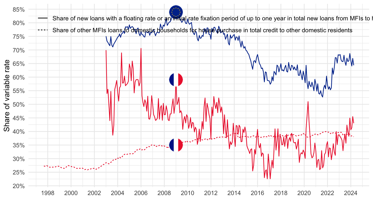
CT1DGGV, SVLHPHH
Code
RAI %>%
  filter(DD_ECON_CONCEPT %in% c("CT1DGGV", "SVLHPHH"),
         REF_AREA %in% c("FR", "U2")) %>%
  left_join(REF_AREA, by = "REF_AREA") %>%
  left_join(DD_ECON_CONCEPT, by = "DD_ECON_CONCEPT") %>%
  month_to_date %>%
  select_if(~n_distinct(.) > 1) %>%
  mutate(Ref_area = ifelse(REF_AREA == "U2", "Europe", Ref_area)) %>%
  left_join(colors, by = c("Ref_area" = "country")) %>%
  mutate(OBS_VALUE = OBS_VALUE/100) %>%
  ggplot(.) + theme_minimal() + xlab("") + ylab("Share of variable rate") +
  geom_line(aes(x = date, y = OBS_VALUE, color = color, linetype = Dd_econ_concept)) +
  add_flags(3) + scale_color_identity() +
  scale_x_date(breaks = seq(1960, 2030, 2) %>% paste0("-01-01") %>% as.Date,
               labels = date_format("%Y")) +
  theme(legend.position = c(0.7, 0.9),
        legend.title = element_blank()) +
  scale_y_continuous(breaks = 0.01*seq(-10, 100, 5),
                     labels = percent_format(accuracy = 1))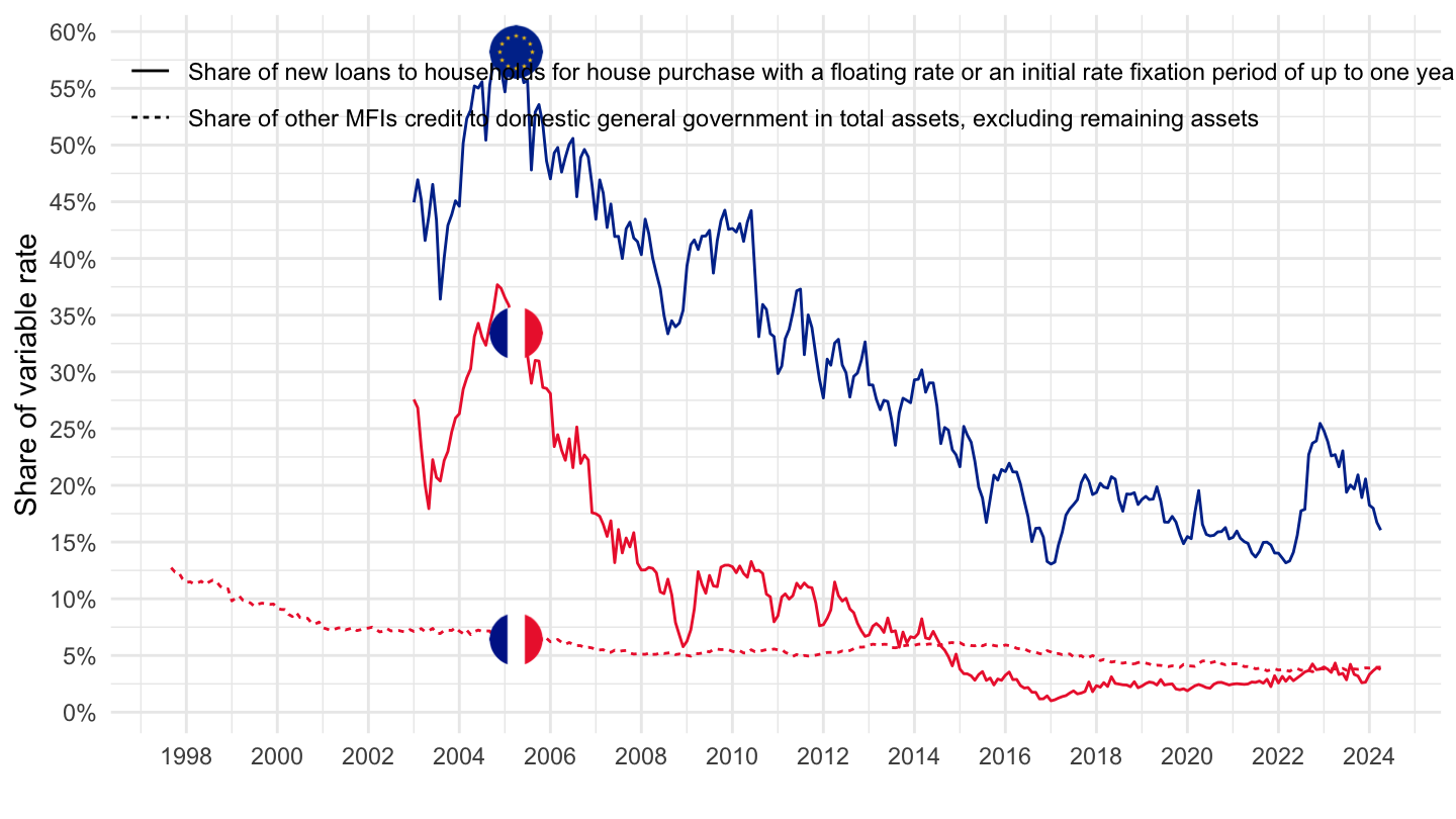
SVLHPHH - Share of floating rates, Households
Table: Last Time
Code
RAI %>%
  filter(DD_ECON_CONCEPT == "SVLHPHH",
         TIME_PERIOD %in% c(last_time)) %>%
  left_join(REF_AREA, by = "REF_AREA") %>%
  select_if(~n_distinct(.) > 1) %>%
  select(REF_AREA, Ref_area, OBS_VALUE, OBS_VALUE) %>%
  mutate(OBS_VALUE = round(OBS_VALUE, 1)) %>%
  mutate(Flag = gsub(" ", "-", str_to_lower(gsub(" ", "-", Ref_area))),
         Flag = paste0('<img src="../../icon/flag/vsmall/', Flag, '.png" alt="Flag">')) %>%
  select(Flag, everything()) %>%
  arrange(OBS_VALUE) %>%
  {if (is_html_output()) datatable(., filter = 'top', rownames = F, escape = F) else .}
Table: Many dates
Code
RAI %>%
  filter(DD_ECON_CONCEPT == "SVLHPHH",
         TIME_PERIOD %in% c(last_time, "2020-01", "2015-01", "2010-01", "2005-01")) %>%
  left_join(REF_AREA, by = "REF_AREA") %>%
  select_if(~n_distinct(.) > 1) %>%
  select(REF_AREA, Ref_area, TIME_PERIOD, OBS_VALUE) %>%
  mutate(OBS_VALUE = round(OBS_VALUE, 1)) %>%
  spread(TIME_PERIOD, OBS_VALUE) %>%
print_table_conditional()| REF_AREA | Ref_area | 2005-01 | 2010-01 | 2015-01 | 2020-01 | 2026-05 |
|---|---|---|---|---|---|---|
| AT | Austria | 65.7 | 76.2 | 87.3 | 40.6 | 18.5 |
| BE | Belgium | 58.2 | 58.4 | 2.4 | 4.5 | 6.1 |
| BG | Bulgaria | NA | 96.2 | 84.0 | 97.3 | 99.4 |
| CY | Cyprus | NA | 61.7 | 95.1 | 90.7 | 17.8 |
| CZ | Czech Republic | NA | NA | 7.2 | 2.1 | 3.5 |
| DE | Germany | 19.1 | 21.6 | 13.2 | 11.6 | 12.0 |
| DK | Denmark | 70.1 | 49.2 | NA | NA | NA |
| EE | Estonia | 99.3 | 56.7 | 85.4 | NA | 97.8 |
| ES | Spain | 93.1 | 90.1 | 66.6 | 32.1 | 7.9 |
| FI | Finland | 97.8 | 97.5 | 96.8 | 97.6 | 95.4 |
| FR | France | 36.5 | 12.8 | 3.8 | 1.9 | 3.3 |
| GR | Greece | 84.4 | 72.2 | 93.1 | 70.2 | 20.7 |
| HR | Croatia | NA | NA | 84.9 | 20.5 | 2.1 |
| HU | Hungary | 58.1 | 84.4 | 44.1 | 2.1 | 7.7 |
| IE | Ireland | 93.6 | 84.1 | 66.0 | 25.8 | 6.3 |
| IT | Italy | 87.3 | 81.3 | 71.7 | 18.0 | 18.7 |
| LT | Lithuania | 97.9 | 84.7 | 89.8 | 97.8 | 86.5 |
| LU | Luxembourg | 88.5 | NA | 63.9 | 30.1 | NA |
| LV | Latvia | 72.3 | 84.4 | NA | 94.3 | 94.0 |
| MT | Malta | NA | 88.0 | 77.9 | 47.4 | NA |
| NL | Netherlands | 43.2 | 24.9 | 19.9 | 17.4 | 18.6 |
| PL | Poland | 90.9 | 100.0 | 99.9 | 100.0 | 28.7 |
| PT | Portugal | 97.8 | 99.5 | 93.0 | 86.7 | 15.8 |
| RO | Romania | NA | NA | 89.9 | 73.6 | 24.8 |
| SE | Sweden | NA | 85.6 | 85.5 | 64.2 | 91.4 |
| SI | Slovenia | 99.1 | 98.1 | 93.4 | 55.5 | 2.0 |
| SK | Slovakia | 62.4 | 36.0 | 6.4 | 1.1 | 1.9 |
| U2 | Euro area (Member States and Institutions of the Euro Area) changing composition | 54.7 | 42.6 | 21.6 | 15.8 | 15.5 |
Netherlands, Germany, Belgium, France, Europe
Code
RAI %>%
  filter(DD_ECON_CONCEPT == "SVLHPHH",
         REF_AREA %in% c("NL", "DE", "BE", "FR",  "U2")) %>%
  left_join(REF_AREA, by = "REF_AREA") %>%
  month_to_date %>%
  select_if(~n_distinct(.) > 1) %>%
  mutate(Ref_area = ifelse(REF_AREA == "U2", "Europe", Ref_area)) %>%
  left_join(colors, by = c("Ref_area" = "country")) %>%
  mutate(OBS_VALUE = OBS_VALUE/100) %>%
  ggplot(.) + theme_minimal() + xlab("") + ylab("Share of variable rate, households (%)") +
  geom_line(aes(x = date, y = OBS_VALUE, color = color)) +
  add_flags(5) + scale_color_identity() +
  scale_x_date(breaks = seq(1960, 2030, 2) %>% paste0("-01-01") %>% as.Date,
               labels = date_format("%Y")) +
  scale_y_continuous(breaks = 0.01*seq(-10, 100, 5),
                     labels = percent_format(accuracy = 1))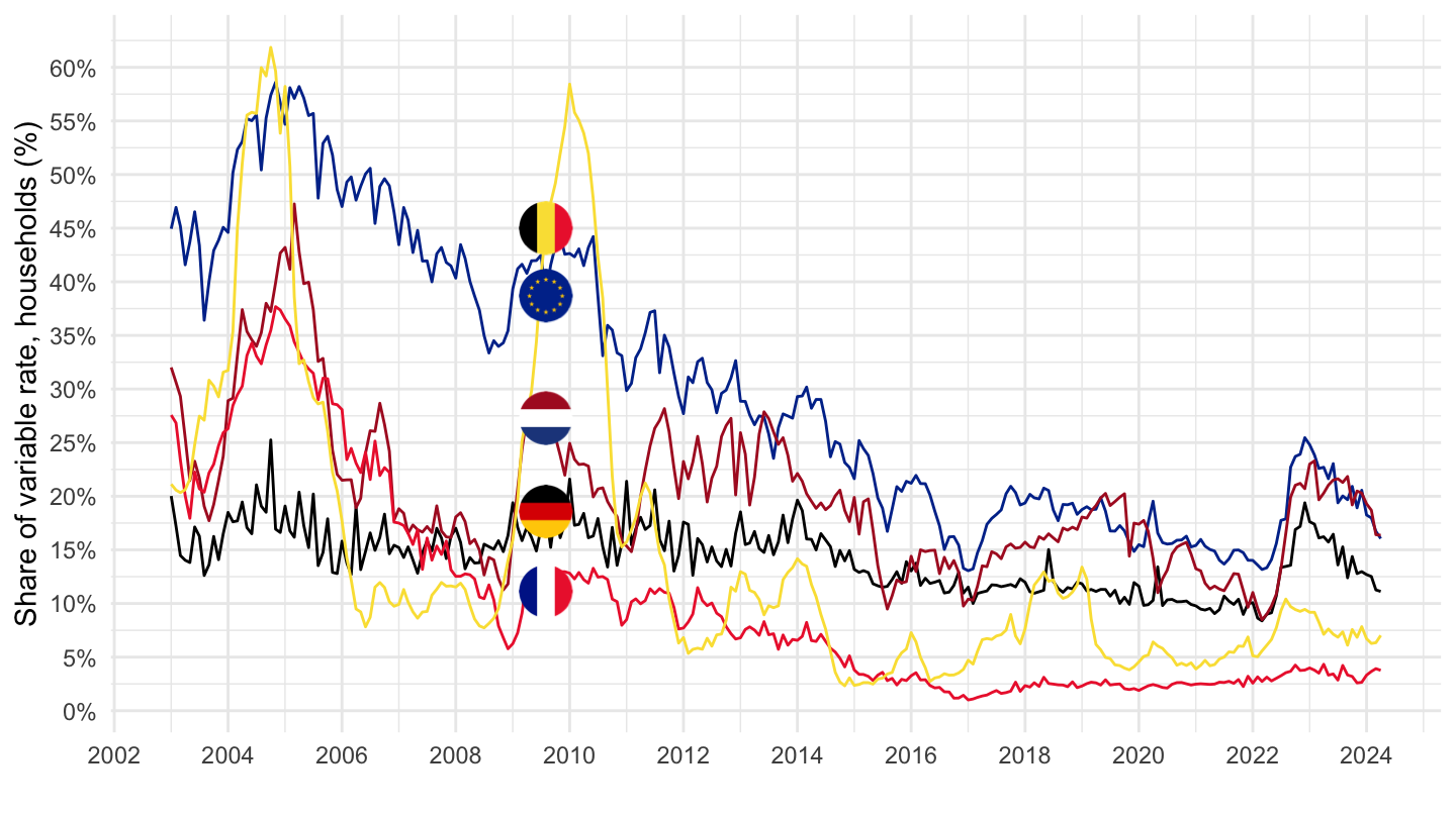
France, Spain, Portugal, latvia, Lithuania, Estonia
Code
RAI %>%
  filter(DD_ECON_CONCEPT == "SVLHPHH",
         REF_AREA %in% c("FR", "ES", "PT", "EE", "LT", "U2")) %>%
  left_join(REF_AREA, by = "REF_AREA") %>%
  month_to_date %>%
  select_if(~n_distinct(.) > 1) %>%
  mutate(Ref_area = ifelse(REF_AREA == "U2", "Europe", Ref_area)) %>%
  left_join(colors, by = c("Ref_area" = "country")) %>%
  mutate(OBS_VALUE = OBS_VALUE/100) %>%
  ggplot(.) + theme_minimal() + xlab("") + ylab("Share of variable rate, households (%)") +
  geom_line(aes(x = date, y = OBS_VALUE, color = color)) +
  add_flags(6) + scale_color_identity() +
  scale_x_date(breaks = seq(1960, 2030, 2) %>% paste0("-01-01") %>% as.Date,
               labels = date_format("%Y")) +
  scale_y_continuous(breaks = 0.01*seq(-10, 100, 5),
                     labels = percent_format(accuracy = 1))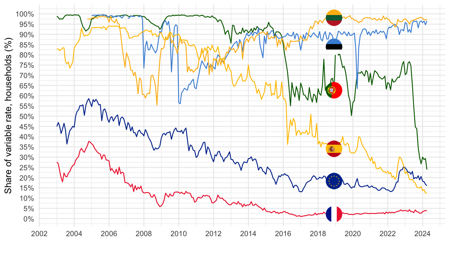
France, Spain, Portugal
Code
RAI %>%
  filter(DD_ECON_CONCEPT == "SVLHPHH",
         REF_AREA %in% c("FR", "ES", "PT")) %>%
  left_join(REF_AREA, by = "REF_AREA") %>%
  month_to_date %>%
  select_if(~n_distinct(.) > 1) %>%
  left_join(colors, by = c("Ref_area" = "country")) %>%
  mutate(OBS_VALUE = OBS_VALUE/100) %>%
  ggplot(.) + theme_minimal() + xlab("") + ylab("Share of variable rate, households (%)") +
  geom_line(aes(x = date, y = OBS_VALUE, color = color)) +
  add_flags(3) + scale_color_identity() +
  scale_x_date(breaks = seq(1960, 2030, 2) %>% paste0("-01-01") %>% as.Date,
               labels = date_format("%Y")) +
  scale_y_continuous(breaks = 0.01*seq(-10, 100, 5),
                     labels = percent_format(accuracy = 1))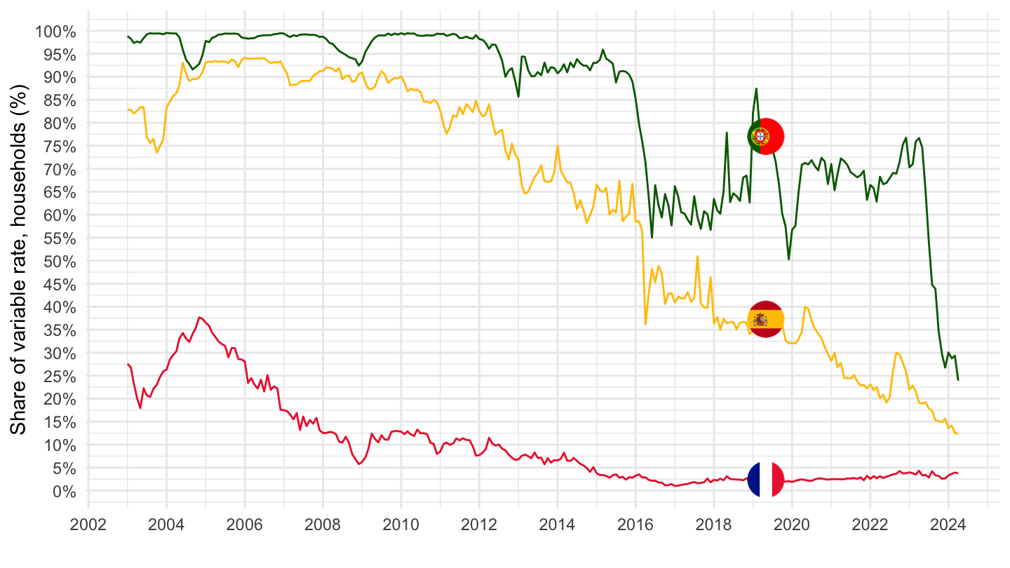
Italy, Sweden, Poland
Code
RAI %>%
  filter(DD_ECON_CONCEPT == "SVLHPHH",
         REF_AREA %in% c("PL", "IT", "SE")) %>%
  left_join(REF_AREA, by = "REF_AREA") %>%
  month_to_date %>%
  select_if(~n_distinct(.) > 1) %>%
  left_join(colors, by = c("Ref_area" = "country")) %>%
  mutate(OBS_VALUE = OBS_VALUE/100) %>%
  ggplot(.) + theme_minimal() + xlab("") + ylab("Share of variable rate, households (%)") +
  geom_line(aes(x = date, y = OBS_VALUE, color = color)) +
  add_flags(3) + scale_color_identity() +
  scale_x_date(breaks = seq(1960, 2030, 2) %>% paste0("-01-01") %>% as.Date,
               labels = date_format("%Y")) +
  scale_y_continuous(breaks = 0.01*seq(-10, 100, 5),
                     labels = percent_format(accuracy = 1))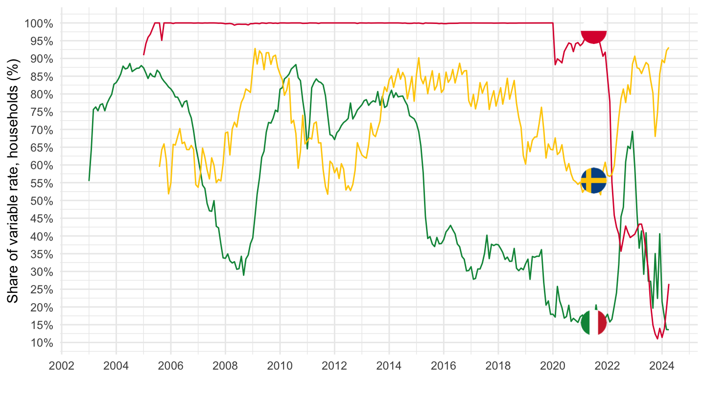
Netherlands, Germany, Belgium
Code
RAI %>%
  filter(DD_ECON_CONCEPT == "SVLHPHH",
         REF_AREA %in% c("NL", "DE", "BE")) %>%
  left_join(REF_AREA, by = "REF_AREA") %>%
  month_to_date %>%
  select_if(~n_distinct(.) > 1) %>%
  left_join(colors, by = c("Ref_area" = "country")) %>%
  mutate(OBS_VALUE = OBS_VALUE/100) %>%
  ggplot(.) + theme_minimal() + xlab("") + ylab("Share of variable rate, households (%)") +
  geom_line(aes(x = date, y = OBS_VALUE, color = color)) +
  add_flags(3) + scale_color_identity() +
  scale_x_date(breaks = seq(1960, 2030, 2) %>% paste0("-01-01") %>% as.Date,
               labels = date_format("%Y")) +
  scale_y_continuous(breaks = 0.01*seq(-10, 100, 5),
                     labels = percent_format(accuracy = 1))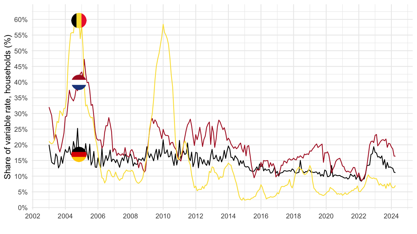
SVLHHNFC - Share of floating rates, Households, and Corporations
Table
Code
RAI %>%
  filter(DD_ECON_CONCEPT == "SVLHHNFC",
         TIME_PERIOD %in% c(last_time, "2020-01", "2015-01", "2010-01", "2005-01")) %>%
  left_join(REF_AREA, by = "REF_AREA") %>%
  select_if(~n_distinct(.) > 1) %>%
  select(REF_AREA, Ref_area, TIME_PERIOD, OBS_VALUE) %>%
  mutate(OBS_VALUE = round(OBS_VALUE, 1)) %>%
  spread(TIME_PERIOD, OBS_VALUE) %>%
print_table_conditional()| REF_AREA | Ref_area | 2005-01 | 2010-01 | 2015-01 | 2020-01 | 2026-05 |
|---|---|---|---|---|---|---|
| AT | Austria | 91.7 | 92.3 | 89.7 | 70.1 | 64.9 |
| BE | Belgium | 90.7 | 90.4 | 76.4 | 73.3 | 74.2 |
| BG | Bulgaria | NA | 98.7 | 95.8 | 95.8 | 98.1 |
| CY | Cyprus | NA | 85.4 | 96.1 | 94.2 | 65.5 |
| CZ | Czech Republic | 80.8 | 76.5 | 51.7 | 48.7 | 32.8 |
| DE | Germany | 61.5 | 72.6 | 59.4 | 61.3 | 66.6 |
| DK | Denmark | 76.4 | 64.5 | 43.6 | 50.2 | 68.6 |
| EE | Estonia | 92.0 | 71.1 | 80.4 | 83.6 | 93.4 |
| ES | Spain | 91.5 | 91.4 | 88.1 | 70.8 | 69.5 |
| FI | Finland | 94.3 | NA | NA | 94.8 | 89.9 |
| FR | France | 64.8 | 45.3 | 39.8 | 32.3 | 38.5 |
| GR | Greece | 82.9 | 86.1 | 97.7 | 91.6 | NA |
| HR | Croatia | NA | NA | 88.8 | 57.8 | 52.1 |
| HU | Hungary | 95.3 | 94.5 | 75.0 | 52.4 | 22.7 |
| IE | Ireland | 83.0 | 87.3 | 82.3 | 67.3 | 55.1 |
| IT | Italy | 90.4 | 93.9 | 92.4 | 73.4 | 76.0 |
| LT | Lithuania | 93.6 | 88.3 | 93.9 | 89.1 | 78.7 |
| LU | Luxembourg | 98.4 | 99.1 | 95.0 | 91.3 | 90.5 |
| LV | Latvia | 72.6 | 82.3 | 80.1 | 95.3 | 91.1 |
| MT | Malta | NA | 98.7 | 89.4 | 59.6 | NA |
| NL | Netherlands | 71.1 | 73.5 | 57.2 | 45.0 | 55.8 |
| PL | Poland | 94.5 | 93.6 | 86.6 | 90.2 | 59.2 |
| PT | Portugal | 95.7 | 95.9 | 90.9 | 74.8 | 47.1 |
| RO | Romania | NA | 96.6 | 85.9 | 67.3 | 54.0 |
| SE | Sweden | NA | 89.2 | 90.6 | 78.7 | 91.4 |
| SI | Slovenia | 89.5 | 93.5 | 91.5 | 78.9 | 56.5 |
| SK | Slovakia | 83.2 | 78.9 | 66.7 | 23.4 | 25.5 |
| U2 | Euro area (Member States and Institutions of the Euro Area) changing composition | 79.2 | 81.5 | 69.9 | 60.5 | 64.4 |
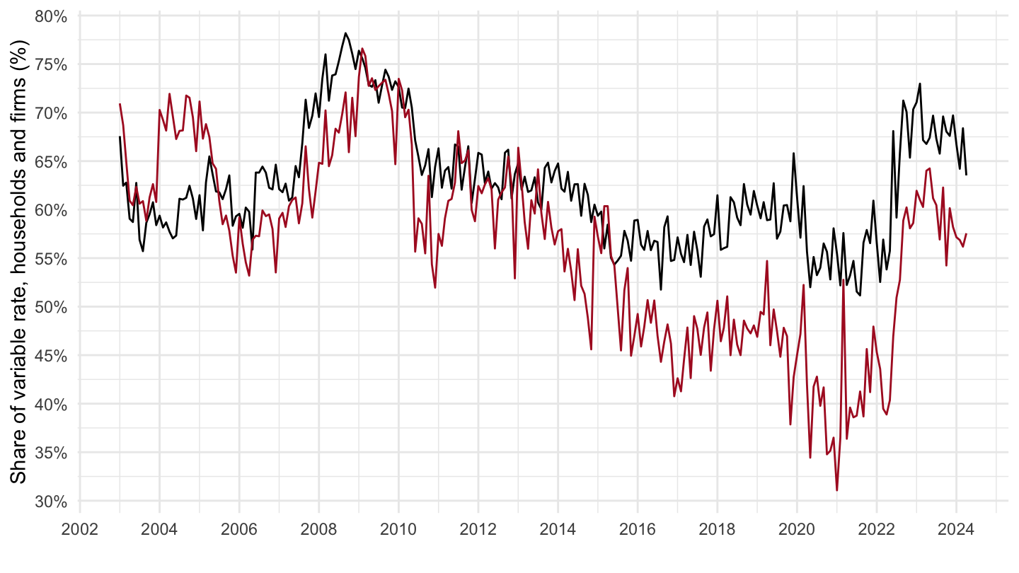
France, Spain, Portugal
Code
RAI %>%
  filter(DD_ECON_CONCEPT == "SVLHHNFC",
         REF_AREA %in% c("FR", "ES", "PT")) %>%
  left_join(REF_AREA, by = "REF_AREA") %>%
  month_to_date %>%
  select_if(~n_distinct(.) > 1) %>%
  left_join(colors, by = c("Ref_area" = "country")) %>%
  mutate(OBS_VALUE = OBS_VALUE/100) %>%
  ggplot(.) + theme_minimal() + xlab("") + ylab("Share of variable rate, households and firms (%)") +
  geom_line(aes(x = date, y = OBS_VALUE, color = color)) +
  add_flags(3) + scale_color_identity() +
  scale_x_date(breaks = seq(1960, 2030, 2) %>% paste0("-01-01") %>% as.Date,
               labels = date_format("%Y")) +
  scale_y_continuous(breaks = 0.01*seq(-10, 100, 5),
                     labels = percent_format(accuracy = 1))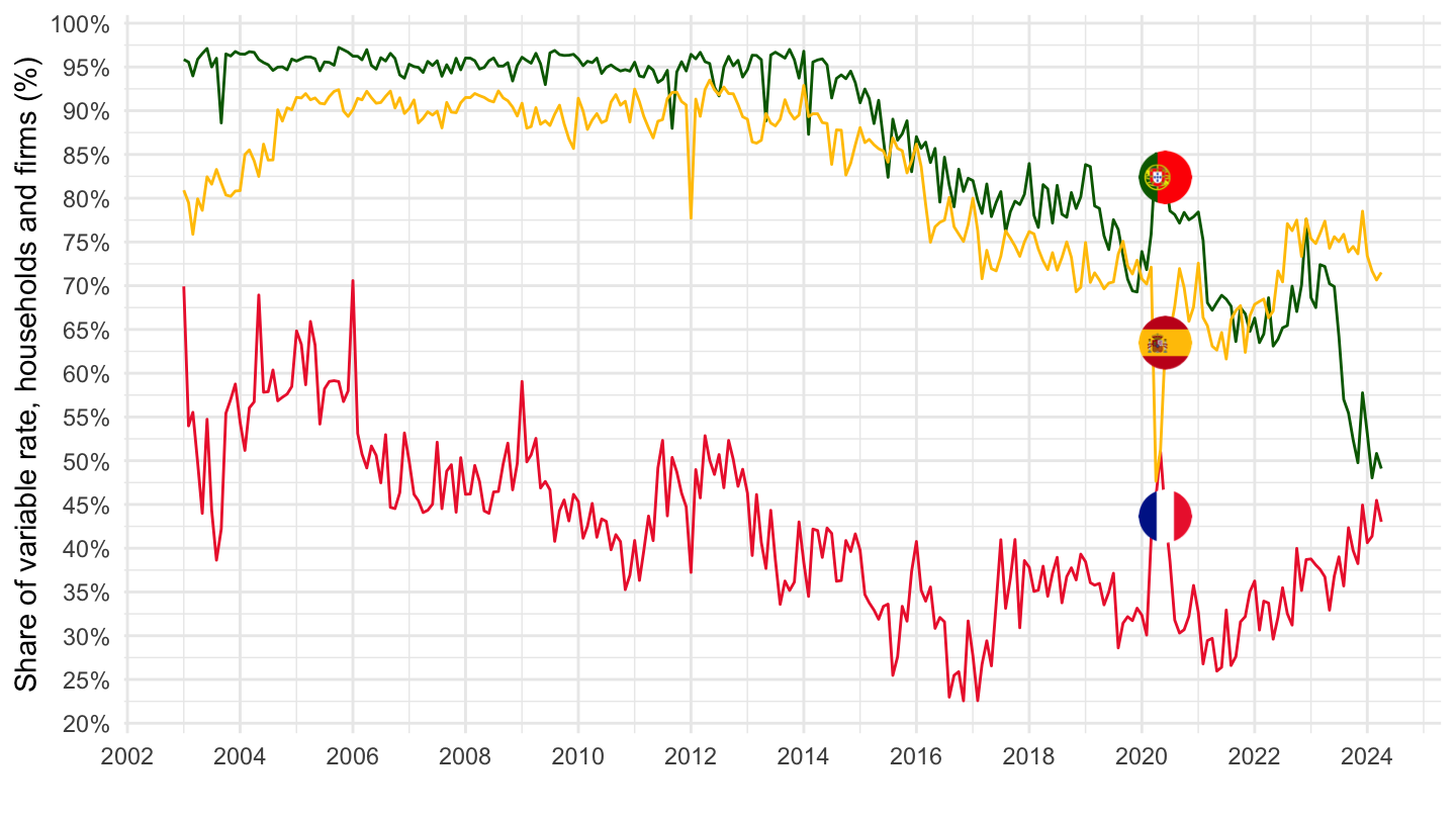
Italy, Sweden, Poland
Code
RAI %>%
  filter(DD_ECON_CONCEPT == "SVLHHNFC",
         REF_AREA %in% c("PL", "IT", "SE")) %>%
  left_join(REF_AREA, by = "REF_AREA") %>%
  month_to_date %>%
  select_if(~n_distinct(.) > 1) %>%
  left_join(colors, by = c("Ref_area" = "country")) %>%
  mutate(OBS_VALUE = OBS_VALUE/100) %>%
  ggplot(.) + theme_minimal() + xlab("") + ylab("Share of variable rate, households and firms (%)") +
  geom_line(aes(x = date, y = OBS_VALUE, color = color)) +
  add_flags(3) + scale_color_identity() +
  scale_x_date(breaks = seq(1960, 2030, 2) %>% paste0("-01-01") %>% as.Date,
               labels = date_format("%Y")) +
  scale_y_continuous(breaks = 0.01*seq(-10, 100, 5),
                     labels = percent_format(accuracy = 1))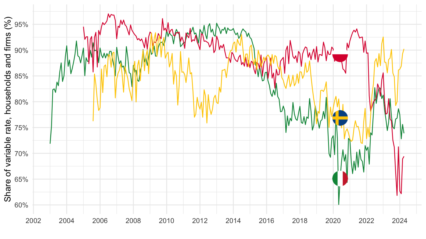
Netherlands, Germany, Belgium
Code
RAI %>%
  filter(DD_ECON_CONCEPT == "SVLHHNFC",
         REF_AREA %in% c("NL", "DE", "BE")) %>%
  left_join(REF_AREA, by = "REF_AREA") %>%
  month_to_date %>%
  select_if(~n_distinct(.) > 1) %>%
  left_join(colors, by = c("Ref_area" = "country")) %>%
  mutate(OBS_VALUE = OBS_VALUE/100) %>%
  ggplot(.) + theme_minimal() + xlab("") + ylab("Share of variable rate, households and firms (%)") +
  geom_line(aes(x = date, y = OBS_VALUE, color = color)) +
  add_flags(3) + scale_color_identity() +
  scale_x_date(breaks = seq(1960, 2030, 2) %>% paste0("-01-01") %>% as.Date,
               labels = date_format("%Y")) +
  scale_y_continuous(breaks = 0.01*seq(-10, 100, 5),
                     labels = percent_format(accuracy = 1))