Money market interest rates - monthly data

Data - Eurostat

Author

François Geerolf

Info

Last observation: Annual: 2026M06 (N = 25)

First observation: Annual: 1970M01 (N = 2)

Last data update: 23 jul 2026, 22:26. Last compile: 24 jul 2026, 02:08

Structure

time

Code

irt_st_m %>%
  group_by(time) %>%
  summarise(Nobs = n()) %>%
  arrange(desc(time)) %>%
  print_table_conditional

Interest Rates

Table

Code

irt_st_m %>%
  filter(int_rt %in% c("IRT_M12"),
         time %in% c("2000M01", "2005M01", "2010M01", "2020M01", "2021M04")) %>%
  select_if(~ n_distinct(.) > 1) %>%
  
  spread(time, values) %>%
  mutate(Geo = ifelse(geo == "DE", "Germany", Geo)) %>%
  mutate(Flag = gsub(" ", "-", str_to_lower(Geo)),
         Flag = paste0('<img src="../../bib/flags/vsmall/', Flag, '.png" alt="Flag">')) %>%
  select(Flag, everything()) %>%
  {if (is_html_output()) datatable(., filter = 'top', rownames = F, escape = F) else .}

UK, SE, DK, EA

All

Code

irt_st_m %>%
  filter(int_rt %in% c("IRT_M12"),
         geo %in% c("UK", "SE", "DK", "EA")) %>%
  
  month_to_date %>%
  mutate(values = values / 100,
         Geo = ifelse(geo == "EA", "Europe", Geo)) %>%
  left_join(colors, by = c("Geo" = "country")) %>%
  ggplot + geom_line(aes(x = date, y = values, color = color)) +
  scale_color_identity() + theme_minimal()  + add_3flags +
  scale_x_date(breaks = as.Date(paste0(seq(1960, 2100, 5), "-01-01")),
               labels = date_format("%Y")) +
  xlab("") + ylab("1 year") +
  scale_y_continuous(breaks = 0.01*seq(-30, 30, 1),
                labels = percent_format(a = 1)) + 
  geom_hline(yintercept = 0, linetype = "dashed",  color = "black")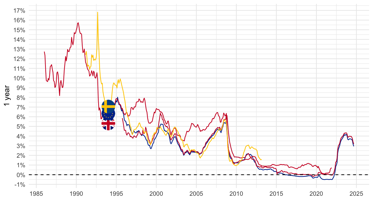

2000-

Code

irt_st_m %>%
  filter(int_rt %in% c("IRT_M12"),
         geo %in% c("UK", "SE", "DK", "EA")) %>%
  
  month_to_date %>%
  filter(date >= as.Date("2000-01-01")) %>%
  mutate(values = values / 100,
         Geo = ifelse(geo == "EA", "Europe", Geo)) %>%
  left_join(colors, by = c("Geo" = "country")) %>%
  ggplot + geom_line(aes(x = date, y = values, color = color)) +
  scale_color_identity() + theme_minimal()  + add_3flags +
  scale_x_date(breaks = as.Date(paste0(seq(1960, 2100, 2), "-01-01")),
               labels = date_format("%Y")) +
  xlab("") + ylab("1 year") +
  scale_y_continuous(breaks = 0.01*seq(-30, 30, 1),
                labels = percent_format(a = 1)) + 
  geom_hline(yintercept = 0, linetype = "dashed",  color = "black")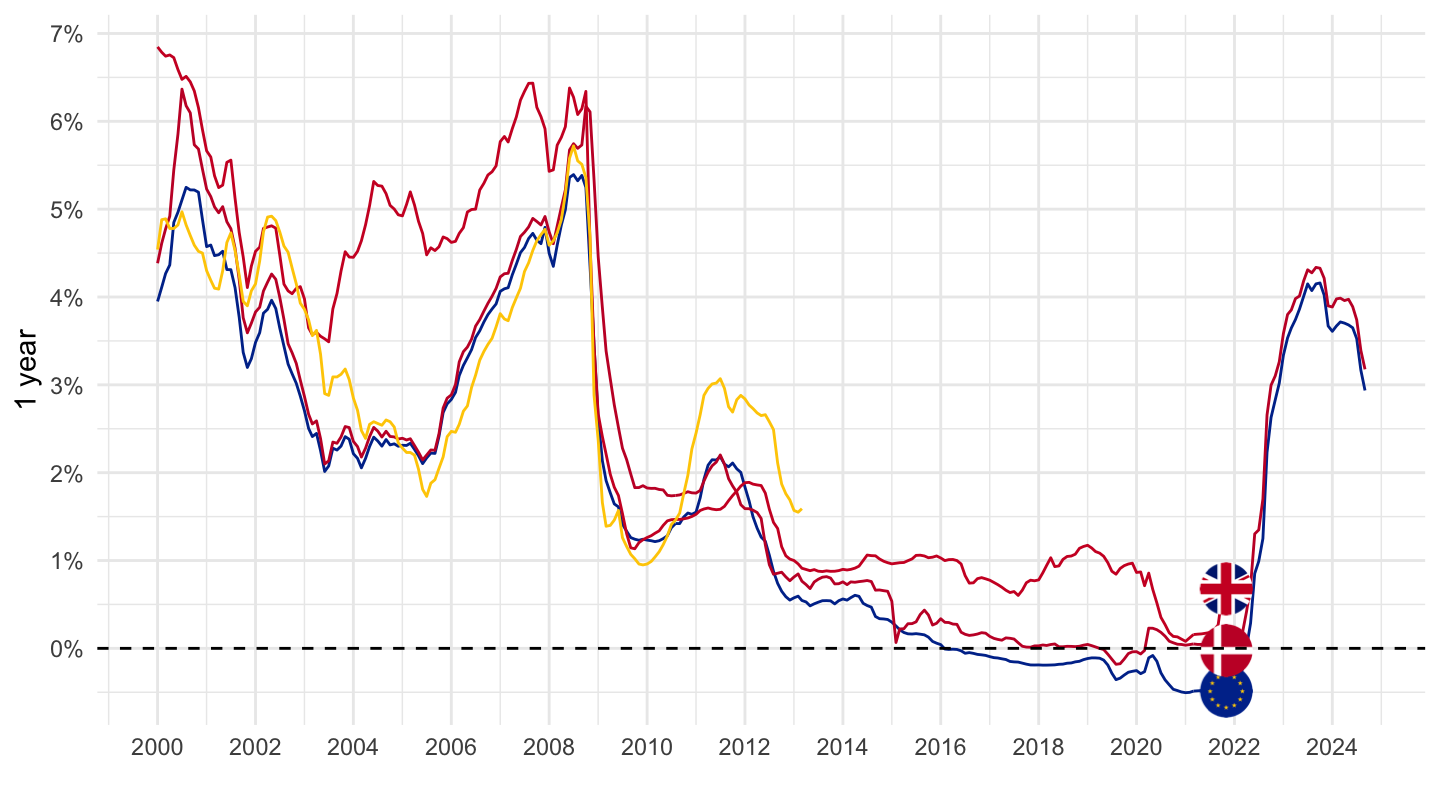

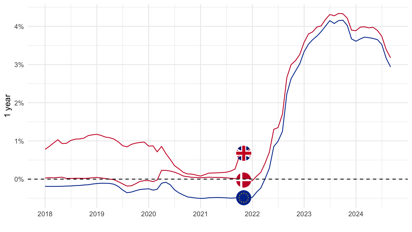
2018-

Code

irt_st_m %>%
  filter(int_rt %in% c("IRT_M12"),
         geo %in% c("UK", "SE", "DK", "EA")) %>%
  
  month_to_date %>%
  filter(date >= as.Date("2018-01-01")) %>%
  mutate(values = values / 100,
         Geo = ifelse(geo == "EA", "Europe", Geo)) %>%
  left_join(colors, by = c("Geo" = "country")) %>%
  ggplot + geom_line(aes(x = date, y = values, color = color)) +
  scale_color_identity() + theme_minimal()  + add_3flags +
  scale_x_date(breaks = as.Date(paste0(seq(1960, 2100, 1), "-01-01")),
               labels = date_format("%Y")) +
  xlab("") + ylab("1 year") +
  scale_y_continuous(breaks = 0.01*seq(-30, 30, 1),
                labels = percent_format(a = 1)) + 
  geom_hline(yintercept = 0, linetype = "dashed",  color = "black")