Monthly Monetary and Financial Statistics (MEI)
Data - OECD
Info
Data on interest rates
| source | dataset | .html | .RData |
|---|---|---|---|
| 2024-07-26 | 2024-06-18 | ||
| 2024-07-26 | 2024-07-01 | ||
| 2024-07-26 | 2024-07-01 | ||
| 2024-09-13 | 2024-05-10 | ||
| 2024-08-09 | 2024-04-19 | ||
| 2024-09-14 | 2024-09-14 | ||
| 2024-06-19 | 2024-09-14 | ||
| 2024-09-14 | 2024-09-14 | ||
| 2024-09-14 | 2024-08-28 | ||
| 2024-09-14 | 2024-09-14 | ||
| 2024-09-14 | 2024-09-14 | ||
| 2024-04-16 | 2024-06-30 | ||
| 2024-09-11 | 2024-05-21 | ||
| 2024-08-28 | 2024-09-15 |
LAST_COMPILE
| LAST_COMPILE |
|---|
| 2024-09-15 |
Last
| obsTime | Nobs |
|---|---|
| 2024-01 | 214 |
Nobs - Javascript
Code
MEI_FIN %>%
  left_join(MEI_FIN_var$SUBJECT, by = "SUBJECT") %>%
  {if (!is_html_output()) mutate(., Subject = substr(Subject, 1, 87)) else .} %>%
  group_by(SUBJECT, Subject, FREQUENCY) %>%
  filter(!is.na(obsValue)) %>%
  summarise(Nobs = n()) %>%
  arrange(-Nobs) %>%
  {if (is_html_output()) datatable(., filter = 'top', rownames = F) else .}
Relative consumer price indices - CCRETT01
FRA, DEU, ITA, USA - Monthly
Code
MEI_FIN %>%
  left_join(MEI_FIN_var$LOCATION, by = "LOCATION") %>%
  filter(SUBJECT == "CCRETT01",
         FREQUENCY == "M",
         LOCATION %in% c("FRA", "DEU", "ITA", "USA")) %>%
  month_to_date %>%
  left_join(colors, by = c("Location" = "country")) %>%
  mutate(color = ifelse(LOCATION == "USA", color2, color)) %>%
  ggplot(.) + geom_line(aes(x = date, y = obsValue, color = color)) +
  theme_minimal() + xlab("") + ylab("Relative consumer price indices") +
  scale_x_date(breaks = seq(1950, 2020, 5) %>% paste0("-01-01") %>% as.Date,
               labels = date_format("%Y")) +
  add_4flags + scale_color_identity() +
  scale_y_continuous(breaks = seq(-10, 300, 10),
                     labels = dollar_format(accuracy = 1, prefix = ""))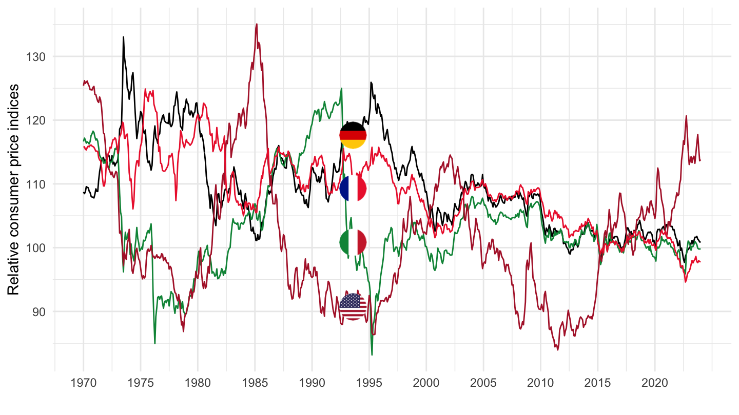
All Countries
Code
MEI_FIN %>%
  left_join(MEI_FIN_var$LOCATION, by = "LOCATION") %>%
  filter(SUBJECT == "CCRETT01") %>%
  group_by(LOCATION, Location, FREQUENCY) %>%
  summarise(Nobs = n(),
            obsTime1 = first(obsTime),
            obsTime2 = last(obsTime)) %>%
  arrange(-Nobs) %>%
  {if (is_html_output()) datatable(., filter = 'top', rownames = F) else .}
LT Interest Rates
France, Germany, Japan
Code
MEI_FIN %>%
  filter(LOCATION %in% c("FRA", "DEU", "JPN"),
         SUBJECT == "IRLT",
         FREQUENCY == "M") %>%
  month_to_date %>%
  filter(date >= as.Date("2010-01-01")) %>%
  left_join(MEI_FIN_var$LOCATION, by = "LOCATION") %>%
  left_join(colors, by = c("Location" = "country")) %>%
  mutate(obsValue = obsValue / 100) %>%
  ggplot(.) + geom_line(aes(x = date, y = obsValue, color = color)) +
  scale_color_identity() +
  theme_minimal() + xlab("") + ylab("Long-Term Interest Rates (%)") +
  add_3flags +
  scale_x_date(breaks = seq(1960, 2024, 1) %>% paste0("-01-01") %>% as.Date,
               labels = date_format("%Y")) +
  scale_y_continuous(breaks = 0.01*seq(-10, 50, 1),
                     labels = percent_format(accuracy = 1)) +
  theme(legend.position = "none") +
  geom_hline(yintercept = 0, linetype = "dashed")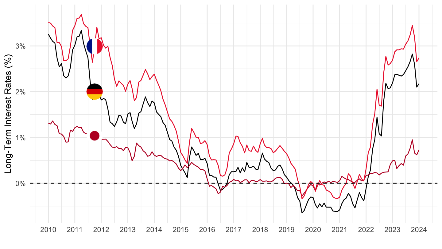
2019-2021
Code
MEI_FIN %>%
  filter(LOCATION %in% c("FRA", "DEU", "JPN"),
         SUBJECT == "IRLT",
         FREQUENCY == "M") %>%
  month_to_date %>%
  filter(date >= as.Date("2014-02-01")) %>%
  left_join(MEI_FIN_var$LOCATION, by = "LOCATION") %>%
  group_by(LOCATION) %>%
  mutate(obsValue = obsValue / 100) %>%
  ggplot(.) + geom_line(aes(x = date, y = obsValue, color = Location)) +
  theme_minimal() + xlab("") + ylab("Taux Nominal sur la Dette, 10 ans (%)") +
  add_3flags +
  scale_x_date(breaks = "1 year",
               labels = date_format("%Y")) +
  scale_y_continuous(breaks = 0.01*seq(-10, 50, .2),
                     labels = percent_format(accuracy = .1)) +
  scale_color_manual(values = c("#002395", "#000000", "#BC002D")) +
  theme(legend.position = "none") +
  geom_hline(yintercept = 0, linetype = "dashed")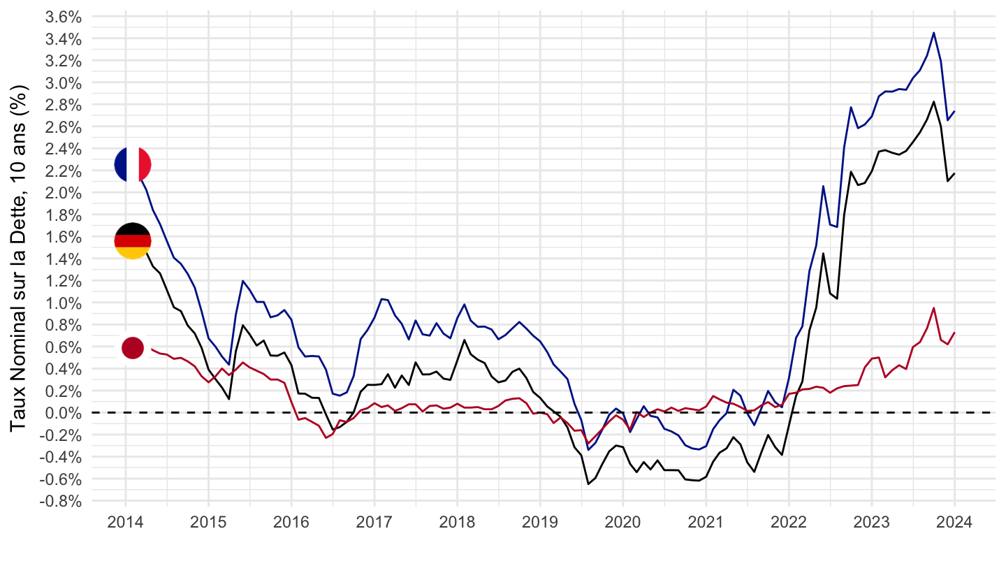
France, United States, Germany, Japan
All
Code
MEI_FIN %>%
  filter(LOCATION %in% c("FRA", "USA", "DEU", "JPN"),
         SUBJECT == "IRLT",
         FREQUENCY == "M") %>%
  month_to_date %>%
  left_join(MEI_FIN_var$LOCATION, by = "LOCATION") %>%
  left_join(colors, by = c("Location" = "country")) %>%
  group_by(LOCATION) %>%
  mutate(obsValue = obsValue / 100) %>%
  ggplot(.) + geom_line(aes(x = date, y = obsValue, color = color)) +
  add_4flags +
  theme_minimal() + xlab("") + ylab("Long-Term Interest Rates (%)") +
  scale_x_date(breaks = seq(1960, 2020, 5) %>% paste0("-01-01") %>% as.Date,
               labels = date_format("%Y")) +
  scale_y_continuous(breaks = 0.01*seq(-10, 50, 1),
                     labels = percent_format(accuracy = 1)) +
  theme(legend.position = c(0.8, 0.80),
        legend.title = element_blank()) +
  scale_color_identity()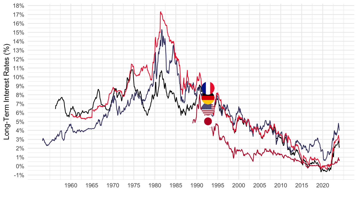
1990-
Code
MEI_FIN %>%
  filter(LOCATION %in% c("FRA", "USA", "DEU", "JPN"),
         SUBJECT == "IRLT",
         FREQUENCY == "M") %>%
  month_to_date %>%
  filter(date >= as.Date("1990-01-01")) %>%
  left_join(MEI_FIN_var$LOCATION, by = "LOCATION") %>%
  left_join(colors, by = c("Location" = "country")) %>%
  group_by(LOCATION) %>%
  mutate(obsValue = obsValue / 100) %>%
  ggplot(.) + geom_line(aes(x = date, y = obsValue, color = color)) +
  scale_color_identity() + add_4flags +
  theme_minimal() + xlab("") + ylab("Long-Term Interest Rates (%)") +
  scale_x_date(breaks = seq(1960, 2020, 5) %>% paste0("-01-01") %>% as.Date,
               labels = date_format("%Y")) +
  scale_y_continuous(breaks = 0.01*seq(-10, 50, 1),
                     labels = percent_format(accuracy = 1)) +
  theme(legend.position = c(0.8, 0.80),
        legend.title = element_blank())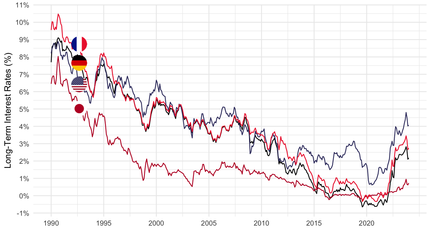
2010-
Code
MEI_FIN %>%
  filter(LOCATION %in% c("FRA", "USA", "DEU", "JPN"),
         SUBJECT == "IRLT",
         FREQUENCY == "M") %>%
  month_to_date %>%
  filter(date >= as.Date("2010-01-01")) %>%
  left_join(MEI_FIN_var$LOCATION, by = "LOCATION") %>%
  left_join(colors, by = c("Location" = "country")) %>%
  group_by(LOCATION) %>%
  ggplot(.) + geom_line(aes(x = date, y = obsValue / 100, color = color)) +
  theme_minimal() + xlab("") + ylab("Long-Term Interest Rates (%)") +
  geom_image(data = . %>%
               filter(date == as.Date("2014-01-01")) %>%
               mutate(image = paste0("../../icon/flag/round/", str_to_lower(gsub(" ", "-", Location)), ".png")),
             aes(x = date, y = obsValue / 100, image = image), asp = 1.5) +
  scale_x_date(breaks = seq(1960, 2024, 1) %>% paste0("-01-01") %>% as.Date,
               labels = date_format("%Y")) +
  scale_y_continuous(breaks = 0.01*seq(-10, 50, 1),
                     labels = percent_format(accuracy = 1)) +
  theme(legend.position = "none") +
  scale_color_identity()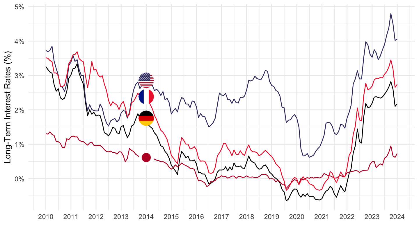
Last 10 years
Code
MEI_FIN %>%
  filter(LOCATION %in% c("FRA", "USA", "DEU", "JPN"),
         SUBJECT == "IRLT",
         FREQUENCY == "M") %>%
  month_to_date %>%
  filter(date >= Sys.Date() - years(10)) %>%
  left_join(MEI_FIN_var$LOCATION, by = "LOCATION") %>%
  left_join(colors, by = c("Location" = "country")) %>%
  group_by(LOCATION) %>%
  ggplot(.) + geom_line(aes(x = date, y = obsValue / 100, color = color)) +
  theme_minimal() + xlab("") + ylab("Long-Term Interest Rates (%)") +
  geom_image(data = . %>%
               filter(date == as.Date("2014-01-01")) %>%
               mutate(image = paste0("../../icon/flag/round/", str_to_lower(gsub(" ", "-", Location)), ".png")),
             aes(x = date, y = obsValue / 100, image = image), asp = 1.5) +
  scale_x_date(breaks = seq(1960, 2024, 1) %>% paste0("-01-01") %>% as.Date,
               labels = date_format("%Y")) +
  scale_y_continuous(breaks = 0.01*seq(-10, 50, 1),
                     labels = percent_format(accuracy = 1)) +
  theme(legend.position = "none") +
  scale_color_identity()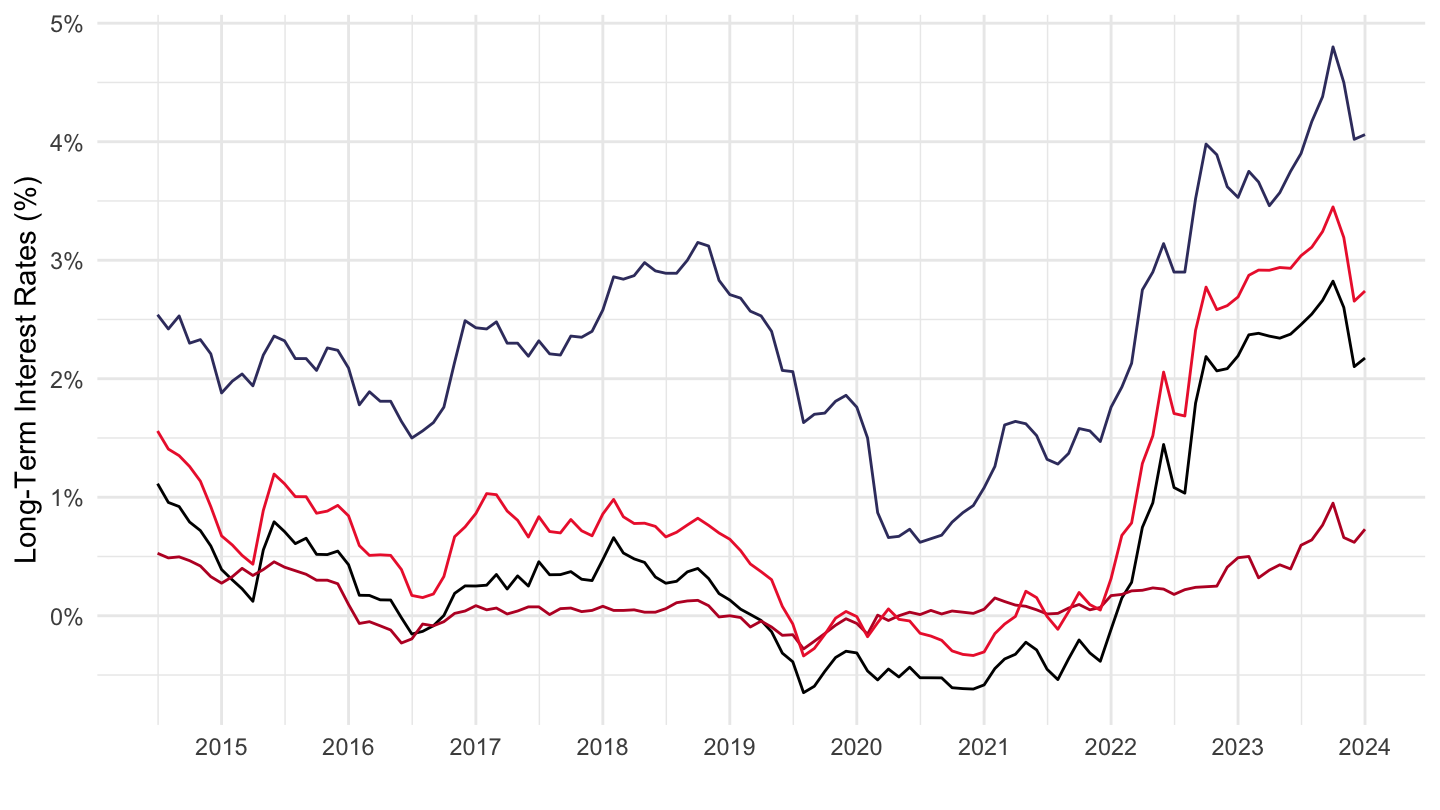
Short-term Rates
France, United States, Germany, Japan
All
Code
MEI_FIN %>%
  filter(LOCATION %in% c("FRA", "USA", "DEU", "JPN"),
         SUBJECT == "IR3TIB",
         FREQUENCY == "M") %>%
  month_to_date %>%
  left_join(MEI_FIN_var$LOCATION, by = "LOCATION") %>%
  left_join(colors, by = c("Location" = "country")) %>%
  group_by(LOCATION) %>%
  mutate(obsValue = obsValue / 100) %>%
  ggplot(.) + geom_line(aes(x = date, y = obsValue, color = color)) +
  add_4flags +
  theme_minimal() + xlab("") + ylab("Short-Term Interest Rates (%)") +
  scale_x_date(breaks = seq(1960, 2020, 5) %>% paste0("-01-01") %>% as.Date,
               labels = date_format("%Y")) +
  scale_y_continuous(breaks = 0.01*seq(-10, 50, 1),
                     labels = percent_format(accuracy = 1)) +
  theme(legend.position = c(0.8, 0.80),
        legend.title = element_blank()) +
  scale_color_identity()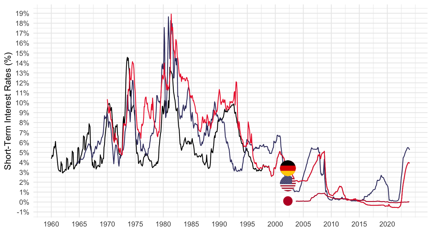
1990-
Code
MEI_FIN %>%
  filter(LOCATION %in% c("FRA", "USA", "DEU", "JPN"),
         SUBJECT == "IR3TIB",
         FREQUENCY == "M") %>%
  month_to_date %>%
  filter(date >= as.Date("1990-01-01")) %>%
  left_join(MEI_FIN_var$LOCATION, by = "LOCATION") %>%
  left_join(colors, by = c("Location" = "country")) %>%
  group_by(LOCATION) %>%
  mutate(obsValue = obsValue / 100) %>%
  ggplot(.) + geom_line(aes(x = date, y = obsValue, color = color)) +
  scale_color_identity() + add_4flags +
  theme_minimal() + xlab("") + ylab("Long-Term Interest Rates (%)") +
  scale_x_date(breaks = seq(1960, 2020, 5) %>% paste0("-01-01") %>% as.Date,
               labels = date_format("%Y")) +
  scale_y_continuous(breaks = 0.01*seq(-10, 50, 1),
                     labels = percent_format(accuracy = 1)) +
  theme(legend.position = c(0.8, 0.80),
        legend.title = element_blank())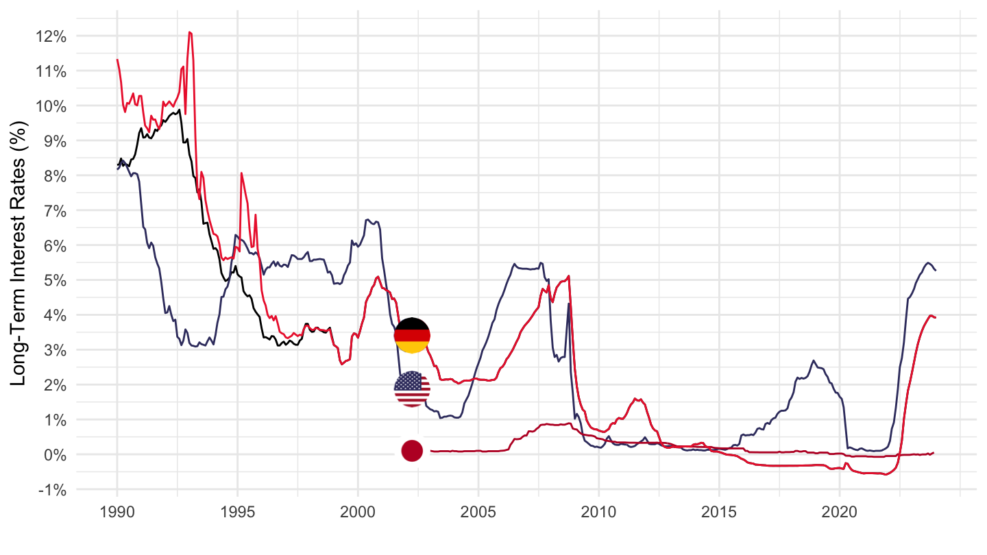
2010-
Code
MEI_FIN %>%
  filter(LOCATION %in% c("FRA", "USA", "DEU", "JPN"),
         SUBJECT == "IR3TIB",
         FREQUENCY == "M") %>%
  month_to_date %>%
  filter(date >= as.Date("2010-01-01")) %>%
  left_join(MEI_FIN_var$LOCATION, by = "LOCATION") %>%
  left_join(colors, by = c("Location" = "country")) %>%
  group_by(LOCATION) %>%
  ggplot(.) + geom_line(aes(x = date, y = obsValue / 100, color = color)) +
  theme_minimal() + xlab("") + ylab("Short-Term Interest Rates (%)") +
  geom_image(data = . %>%
               filter(date == as.Date("2014-01-01")) %>%
               mutate(image = paste0("../../icon/flag/round/", str_to_lower(gsub(" ", "-", Location)), ".png")),
             aes(x = date, y = obsValue / 100, image = image), asp = 1.5) +
  scale_x_date(breaks = seq(1960, 2024, 1) %>% paste0("-01-01") %>% as.Date,
               labels = date_format("%Y")) +
  scale_y_continuous(breaks = 0.01*seq(-10, 50, 1),
                     labels = percent_format(accuracy = 1)) +
  theme(legend.position = "none") +
  scale_color_identity()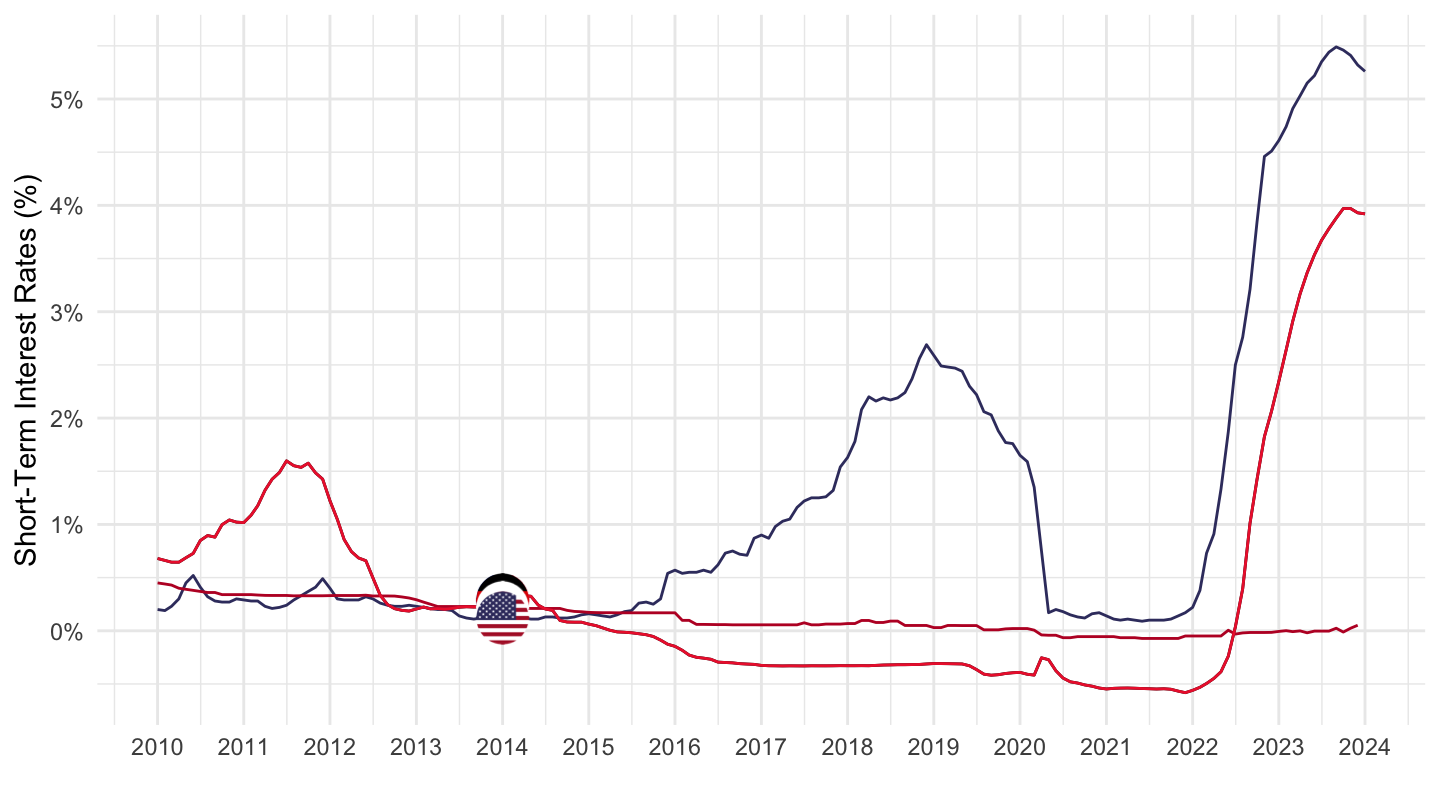
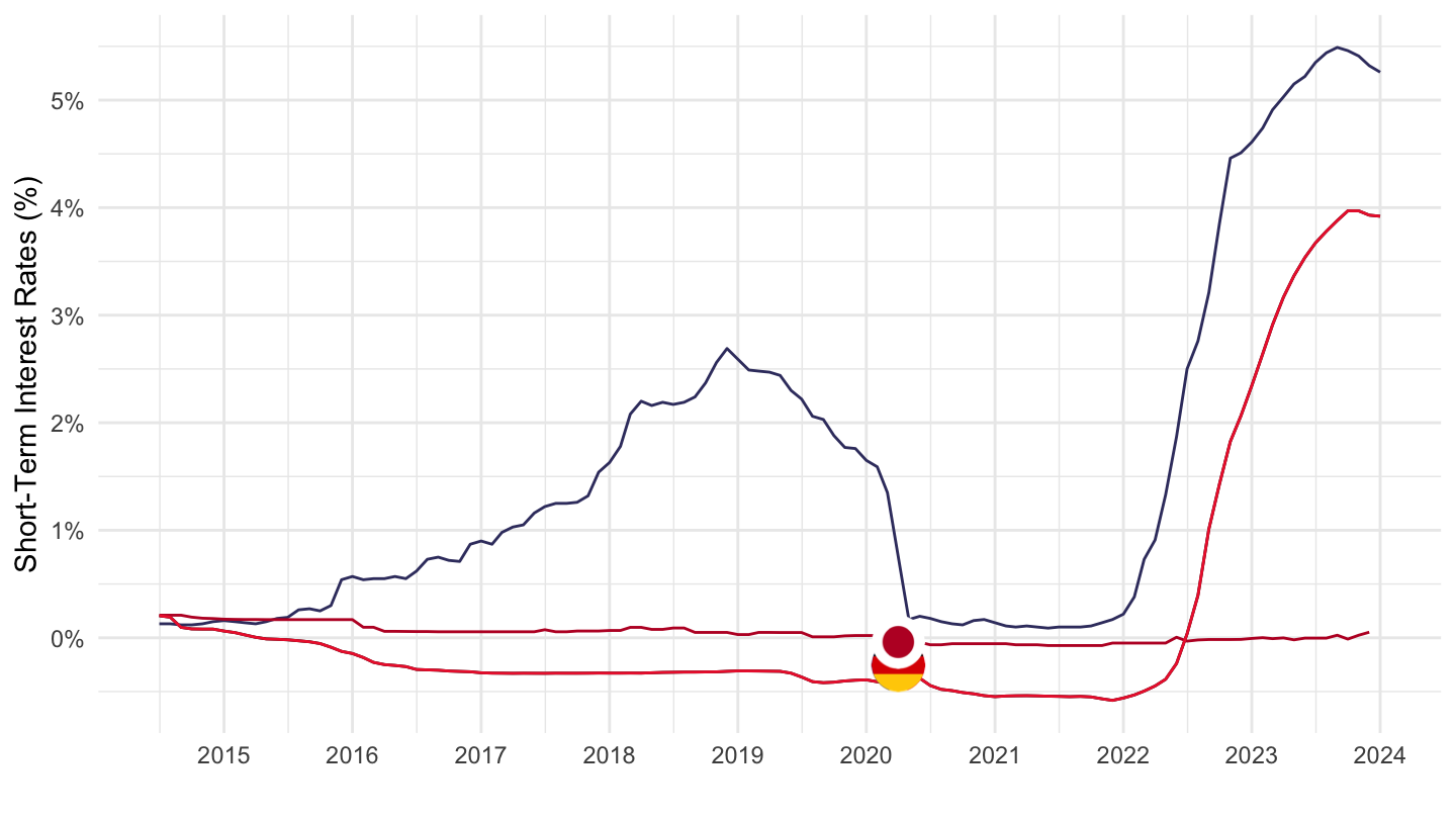
Last 10 years
Code
MEI_FIN %>%
  filter(LOCATION %in% c("FRA", "USA", "DEU", "JPN"),
         SUBJECT == "IR3TIB",
         FREQUENCY == "M") %>%
  month_to_date %>%
  filter(date >= Sys.Date() - years(10)) %>%
  left_join(MEI_FIN_var$LOCATION, by = "LOCATION") %>%
  left_join(colors, by = c("Location" = "country")) %>%
  group_by(LOCATION) %>%
  mutate(obsValue = obsValue / 100) %>%
  ggplot(.) + geom_line(aes(x = date, y = obsValue, color = color)) +
  theme_minimal() + xlab("") + ylab("Short-Term Interest Rates (%)") + add_3flags +
  scale_x_date(breaks = seq(1960, 2024, 1) %>% paste0("-01-01") %>% as.Date,
               labels = date_format("%Y")) +
  scale_y_continuous(breaks = 0.01*seq(-10, 50, 1),
                     labels = percent_format(accuracy = 1)) +
  theme(legend.position = "none") +
  scale_color_identity()