Internal Liquidity Management
Data - ECB
Info
Data on monetary policy
| source | dataset | Title | .html | .rData |
|---|---|---|---|---|
| ecb | ILM | Internal Liquidity Management | 2026-07-23 | 2026-07-22 |
| bdf | FM | Marché financier, taux | 2026-07-22 | 2026-07-22 |
| bdf | MIR | Taux d'intérêt - Zone euro | 2026-07-22 | 2026-07-22 |
| bdf | MIR1 | Taux d'intérêt - France | 2026-07-23 | 2026-07-23 |
| bis | CBPOL | Policy Rates, Daily | 2026-07-18 | 2026-07-22 |
| ecb | BSI | Balance Sheet Items | 2026-07-23 | 2026-07-22 |
| ecb | BSI_PUB | Balance Sheet Items - Published series | 2026-07-23 | 2026-07-22 |
| ecb | FM | Financial market data | 2026-07-23 | 2026-07-22 |
| ecb | ILM_PUB | Internal Liquidity Management - Published series | 2026-07-23 | 2026-07-22 |
| ecb | MIR | MFI Interest Rate Statistics | 2026-07-23 | 2026-07-22 |
| ecb | RAI | Risk Assessment Indicators | 2026-07-23 | 2026-07-23 |
| ecb | SUP | Supervisory Banking Statistics | 2026-07-23 | 2026-07-23 |
| ecb | YC | Financial market data - yield curve | 2026-07-23 | 2026-07-23 |
| ecb | YC_PUB | Financial market data - yield curve - Published series | 2026-07-23 | 2026-07-23 |
| ecb | liq_daily | Daily Liquidity | 2026-07-23 | 2026-07-23 |
| eurostat | ei_mfir_m | Interest rates - monthly data | 2026-07-23 | 2026-07-23 |
| eurostat | irt_st_m | Money market interest rates - monthly data | 2026-07-23 | 2026-07-23 |
| fred | r | Interest Rates | 2026-07-22 | 2026-07-22 |
| oecd | MEI | Main Economic Indicators | 2024-04-16 | 2025-07-24 |
| oecd | MEI_FIN | Monthly Monetary and Financial Statistics (MEI) | 2024-09-15 | 2025-07-24 |
LAST_COMPILE
| LAST_COMPILE |
|---|
| 2026-07-24 |
Last
Code
ILM %>%
  group_by(TIME_PERIOD, FREQ) %>%
  summarise(Nobs = n()) %>%
  arrange(desc(TIME_PERIOD)) %>%
  head(5) %>%
print_table_conditional()| TIME_PERIOD | FREQ | Nobs |
|---|---|---|
| 2026-W29 | W | 43 |
| 2026-W28 | W | 43 |
| 2026-W27 | W | 43 |
| 2026-W26 | W | 43 |
| 2026-W25 | W | 43 |
Info
- Liquidity. html
FREQ
Code
ILM %>%
  left_join(FREQ,  by = "FREQ") %>%
  group_by(FREQ, Freq) %>%
  summarise(Nobs = n()) %>%
  arrange(-Nobs) %>%
{if (is_html_output()) print_table(.) else .}| FREQ | Freq | Nobs |
|---|---|---|
| M | Monthly | 140542 |
| W | Weekly | 49371 |
| D | Daily | 24917 |
REF_AREA
Code
ILM %>%
  left_join(REF_AREA,  by = "REF_AREA") %>%
  group_by(REF_AREA, Ref_area) %>%
  summarise(Nobs = n()) %>%
  arrange(-Nobs) %>%
  {if (is_html_output()) datatable(., filter = 'top', rownames = F) else .}
BS_REP_SECTOR
Code
ILM %>%
  left_join(BS_REP_SECTOR,  by = "BS_REP_SECTOR") %>%
  group_by(BS_REP_SECTOR, Bs_rep_sector) %>%
  summarise(Nobs = n()) %>%
  arrange(-Nobs) %>%
  {if (is_html_output()) datatable(., filter = 'top', rownames = F) else .}
BS_ITEM
Code
ILM %>%
  left_join(BS_ITEM,  by = "BS_ITEM") %>%
  group_by(BS_ITEM, Bs_item) %>%
  summarise(Nobs = n()) %>%
  {if (is_html_output()) datatable(., filter = 'top', rownames = F) else .}
KEY
Code
ILM %>%
  group_by(KEY, TITLE) %>%
  summarise(Nobs = n()) %>%
  mutate(KEY = paste0('<a  target=_blank href=https://data.ecb.europa.eu/data/datasets/ILM/', KEY, ' >', KEY, '</a>')) %>%
  {if (is_html_output()) datatable(., filter = 'top', rownames = F, escape = F) else .}
Daily
List of datasets
Code
ILM %>%
  filter(FREQ == "D") %>%
  group_by(KEY, TITLE) %>%
  summarise(Nobs = n()) %>%
  mutate(KEY = paste0("[", KEY, "](https://data.ecb.europa.eu/data/datasets/ILM/", KEY, ')')) %>%
print_table_conditional()| KEY | TITLE | Nobs |
|---|---|---|
| [ILM.D.U2.C.A050500.U2.EUR] | https://data.ecb.europa.eu/data/datasets/ILM/ILM.D.U2.C.A050500.U2.EUR)| | |
| [ILM.D.U2.C.BMK1.U2.EUR](ht | ps://data.ecb.europa.eu/data/datasets/ILM/ILM.D.U2.C.BMK1.U2.EUR)| Be | chmark |
| [ILM.D.U2.C.EXLIQ.U2.EUR](h | tps://data.ecb.europa.eu/data/datasets/ILM/ILM.D.U2.C.EXLIQ.U2.EUR)| | |
| [ILM.D.U2.C.FAAF1.Z5.Z01](h | tps://data.ecb.europa.eu/data/datasets/ILM/ILM.D.U2.C.FAAF1.Z5.Z01)| | |
| [ILM.D.U2.C.FAAF2.Z5.Z01](h | tps://data.ecb.europa.eu/data/datasets/ILM/ILM.D.U2.C.FAAF2.Z5.Z01)| | |
| [ILM.D.U2.C.L020100.U2.EUR] | https://data.ecb.europa.eu/data/datasets/ILM/ILM.D.U2.C.L020100.U2.EUR)| | |
| [ILM.D.U2.C.L020200.U2.EUR] | https://data.ecb.europa.eu/data/datasets/ILM/ILM.D.U2.C.L020200.U2.EUR)| | |
| [ILM.D.U2.C.MRR.U2.EUR](htt | s://data.ecb.europa.eu/data/datasets/ILM/ILM.D.U2.C.MRR.U2.EUR)| | Mini |
| [ILM.D.U2.C.NLIQ.U2.EUR](ht | ps://data.ecb.europa.eu/data/datasets/ILM/ILM.D.U2.C.NLIQ.U2.EUR)| Net liquidity | ffect |
| [ILM.D.U2.C.TOMO.U2.EUR](ht | ps://data.ecb.europa.eu/data/datasets/ILM/ILM.D.U2.C.TOMO.U2.EUR)| Open | market |
Main Refinancing operation
France, Germany, Italy
Code
ILM %>%
  filter(KEY %in% c("ILM.M.FR.N.A050100.U2.EUR",
                    "ILM.M.DE.N.A050100.U2.EUR",
                    "ILM.M.IT.N.A050100.U2.EUR")) %>%
  month_to_date %>%
  mutate(OBS_VALUE = OBS_VALUE/1000) %>%
  ggplot + geom_line(aes(x = date, y = OBS_VALUE, color = TITLE)) +
  ylab("") + xlab("") + theme_minimal() +
  theme(legend.position = c(0.45, 0.9),
        legend.title = element_blank()) +
  scale_y_continuous(breaks = seq(0, 10000, 2),
                labels = dollar_format(acc = 1, pre = "", su = " Bn€")) +
  scale_x_date(breaks = as.Date(paste0(seq(1940, 2100,  1), "-01-01")),
               labels = date_format("%Y"))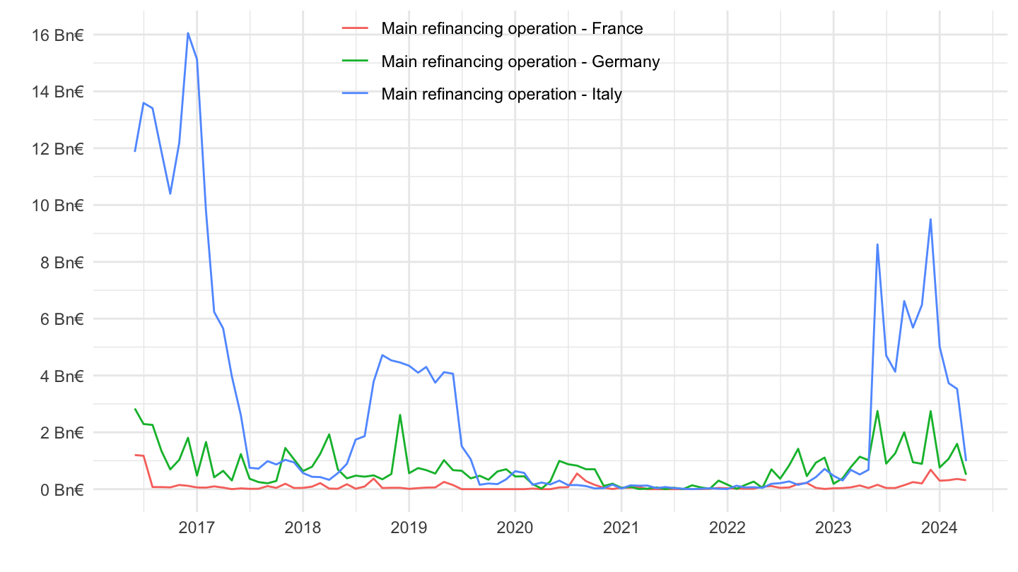
Eurosystem
Monthly
Code
ILM %>%
  filter(KEY %in% c("ILM.M.U2.C.A050100.U2.EUR")) %>%
  month_to_date %>%
  mutate(OBS_VALUE = OBS_VALUE/1000) %>%
  ggplot + geom_line(aes(x = date, y = OBS_VALUE, color = TITLE)) +
  ylab("") + xlab("") + theme_minimal() +
  theme(legend.position = c(0.45, 0.9),
        legend.title = element_blank()) +
  scale_y_continuous(breaks = seq(0, 10000, 20),
                labels = dollar_format(acc = 1, pre = "", su = " Bn€")) +
  scale_x_date(breaks = as.Date(paste0(seq(1940, 2100,  2), "-01-01")),
               labels = date_format("%Y"))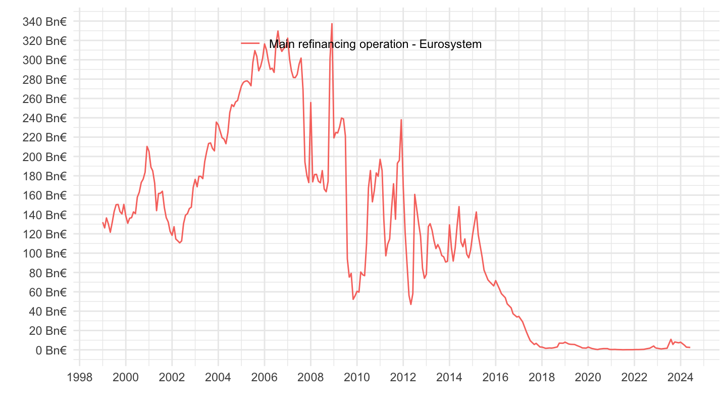
Weekly
Code
ILM %>%
  filter(KEY %in% c("ILM.W.U2.C.A050100.U2.EUR")) %>%
  arrange(desc(TIME_PERIOD)) %>%
  week_to_date %>%
  mutate(OBS_VALUE = OBS_VALUE/1000) %>%
  ggplot + geom_line(aes(x = date, y = OBS_VALUE)) +
  ylab("Main refinancing operation - Eurosystem") + xlab("") + theme_minimal() +
  theme(legend.position = c(0.45, 0.9),
        legend.title = element_blank()) +
  scale_y_continuous(breaks = seq(0, 10000, 20),
                labels = dollar_format(acc = 1, pre = "", su = " Bn€")) +
  scale_x_date(breaks = as.Date(paste0(seq(1940, 2100,  2), "-01-01")),
               labels = date_format("%Y"))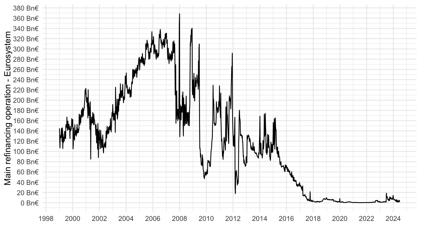
Total Assets
France, Germany, Italy
Code
ILM %>%
  filter(KEY %in% c("ILM.M.DE.N.T000000.Z5.Z01",
                    "ILM.M.FR.N.T000000.Z5.Z01",
                    "ILM.M.IT.N.T000000.Z5.Z01")) %>%
  month_to_date %>%
  mutate(OBS_VALUE = OBS_VALUE/1000) %>%
  ggplot + geom_line(aes(x = date, y = OBS_VALUE, color = TITLE)) +
  ylab("") + xlab("") + theme_minimal() +
  theme(legend.position = c(0.45, 0.9),
        legend.title = element_blank()) +
  scale_y_continuous(breaks = seq(0, 10000, 200),
                labels = dollar_format(acc = 1, pre = "", su = " Bn€")) +
  scale_x_date(breaks = as.Date(paste0(seq(1940, 2100,  1), "-01-01")),
               labels = date_format("%Y"))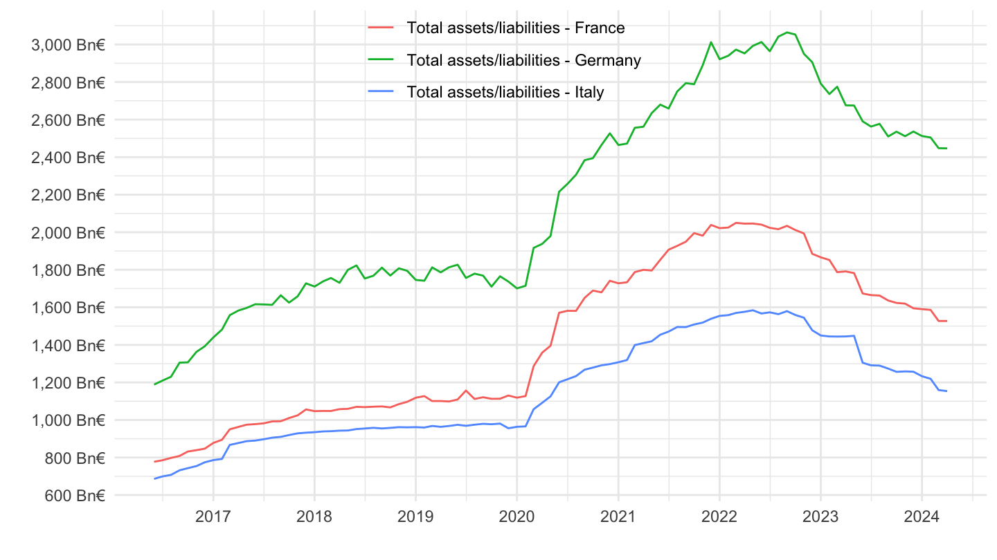
France, Germany, Italy
Code
ILM %>%
  filter(KEY %in% c("ILM.M.FR.N.L020000.U2.EUR",
                    "ILM.M.DE.N.L020000.U2.EUR",
                    "ILM.M.IT.N.L020000.U2.EUR")) %>%
  month_to_date %>%
  mutate(OBS_VALUE = OBS_VALUE/1000) %>%
  ggplot + geom_line(aes(x = date, y = OBS_VALUE, color = TITLE)) +
  ylab("") + xlab("") + theme_minimal() +
  theme(legend.position = c(0.45, 0.9),
        legend.title = element_blank()) +
  scale_y_continuous(breaks = seq(0, 10000, 200),
                labels = dollar_format(acc = 1, pre = "", su = " Bn€")) +
  scale_x_date(breaks = as.Date(paste0(seq(1940, 2100,  1), "-01-01")),
               labels = date_format("%Y"))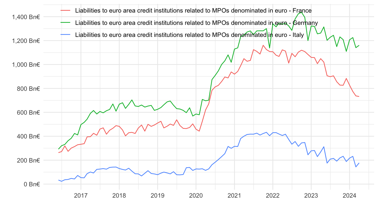
Liabilities to euro area credit institutions related to monetary policy operations denominated in euro
Base money
Linear
Code
ILM %>%
  filter(KEY %in% c("ILM.M.U2.C.LT00001.Z5.EUR",
                    "ILM.M.U2.C.L020100.U2.EUR")) %>%
  month_to_date %>%
  mutate(OBS_VALUE = OBS_VALUE/1000) %>%
  ggplot + geom_line(aes(x = date, y = OBS_VALUE, color = TITLE)) +
  ylab("") + xlab("") + theme_minimal() +
  theme(legend.position = c(0.45, 0.9),
        legend.title = element_blank()) +
  scale_y_continuous(breaks = seq(0, 10000, 500),
                labels = dollar_format(acc = 1, pre = "", su = " Bn€")) +
  scale_x_date(breaks = as.Date(paste0(seq(1940, 2100,  2), "-01-01")),
               labels = date_format("%Y"))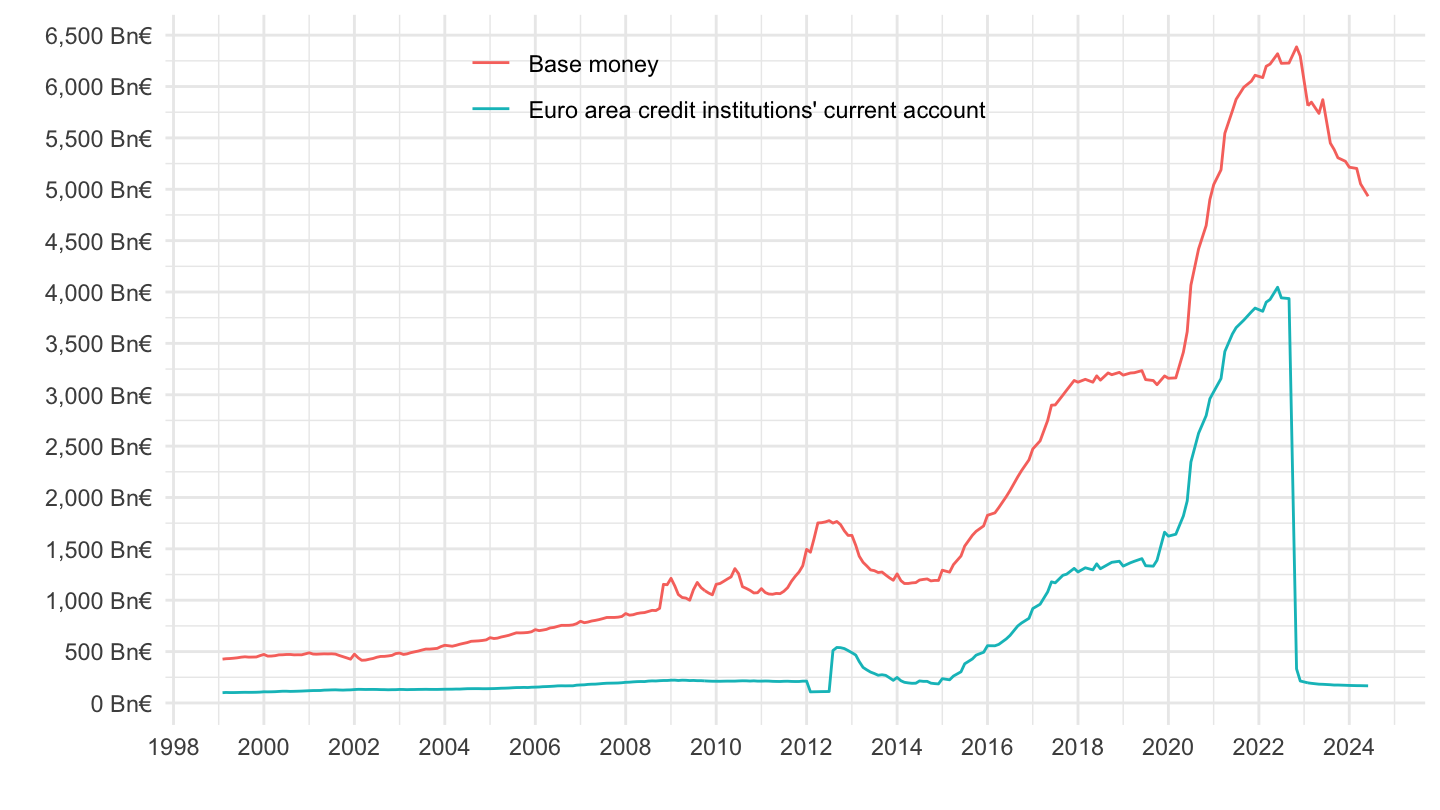
Log
Code
ILM %>%
  filter(KEY %in% c("ILM.M.U2.C.LT00001.Z5.EUR",
                    "ILM.M.U2.C.L020100.U2.EUR")) %>%
  month_to_date %>%
  mutate(OBS_VALUE = OBS_VALUE/1000) %>%
  ggplot + geom_line(aes(x = date, y = OBS_VALUE, color = TITLE)) +
  ylab("Required and Excess reserves") + xlab("") + theme_minimal() +
  theme(legend.position = c(0.45, 0.9),
        legend.title = element_blank()) +
  scale_y_log10(breaks = 10^(seq(0, 10, 1)),
                labels = dollar_format(acc = 1, pre = "", su = " Bn€")) +
  scale_x_date(breaks = as.Date(paste0(seq(1940, 2100,  2), "-01-01")),
               labels = date_format("%Y"))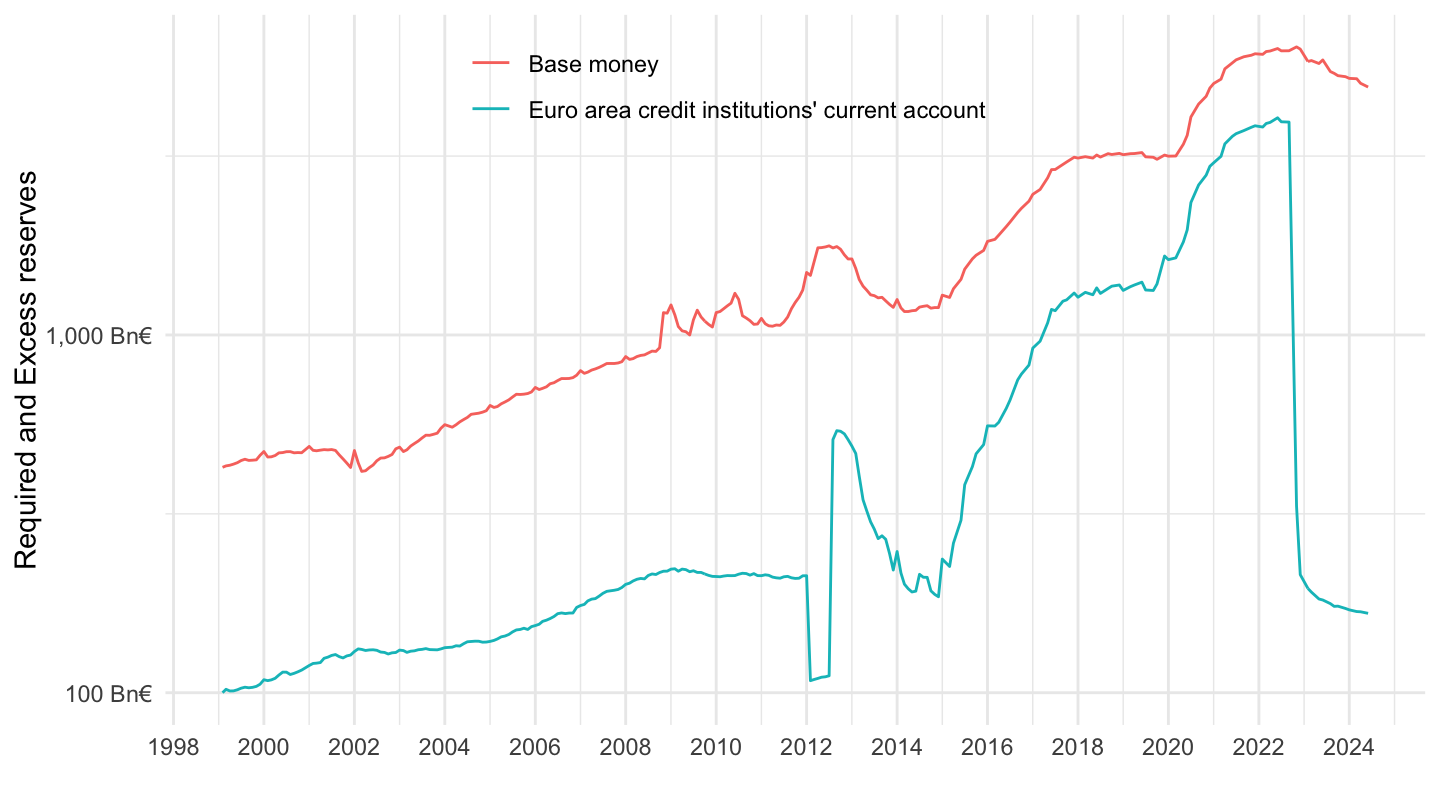
Banknotes in circulation - Differences
Code
ILM %>%
  filter(KEY %in% c("ILM.M.4F.E.L010000.Z5.EUR",
                    "ILM.M.U2.C.L010000.Z5.EUR")) %>%
  month_to_date %>%
  mutate(OBS_VALUE = OBS_VALUE/1000) %>%
  ggplot + geom_line(aes(x = date, y = OBS_VALUE, color = TITLE)) +
  ylab("Liquidity-providing factors") + xlab("") + theme_minimal() +
  theme(legend.position = c(0.45, 0.8),
        legend.title = element_blank()) +
  scale_y_continuous(breaks = seq(0, 10000, 200),
                labels = dollar_format(acc = 1, pre = "", su = " Bn€")) +
  scale_x_date(breaks = as.Date(paste0(seq(1940, 2100,  2), "-01-01")),
               labels = date_format("%Y"))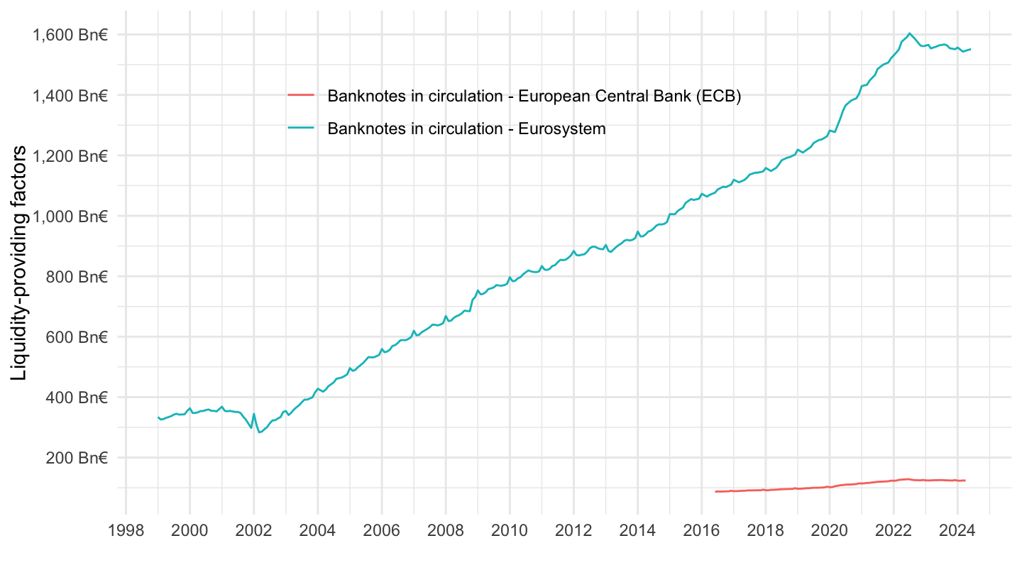
Liquidity
https://data.ecb.europa.eu/publications/ecbeurosystem-policy-and-exchange-rates/3030613
Liquidity-providing factors
Individual
Bn€
Code
ILM %>%
  filter(KEY %in% c("ILM.M.U2.C.AN00001.Z5.Z0Z",
                    "ILM.M.U2.C.A050100.U2.EUR",
                    "ILM.M.U2.C.A050200.U2.EUR",
                    "ILM.M.U2.C.A050500.U2.EUR",
                    "ILM.M.U2.C.A050A00.U2.EUR")) %>%
  month_to_date %>%
  mutate(OBS_VALUE = OBS_VALUE/1000) %>%
  ggplot + geom_line(aes(x = date, y = OBS_VALUE, color = TITLE)) +
  ylab("Liquidity-providing factors
") + xlab("") + theme_minimal() +
  theme(legend.position = c(0.45, 0.8),
        legend.title = element_blank()) +
  scale_y_continuous(breaks = seq(0, 10000, 500),
                labels = dollar_format(acc = 1, pre = "", su = " Bn€")) +
  scale_x_date(breaks = as.Date(paste0(seq(1940, 2100,  2), "-01-01")),
               labels = date_format("%Y"))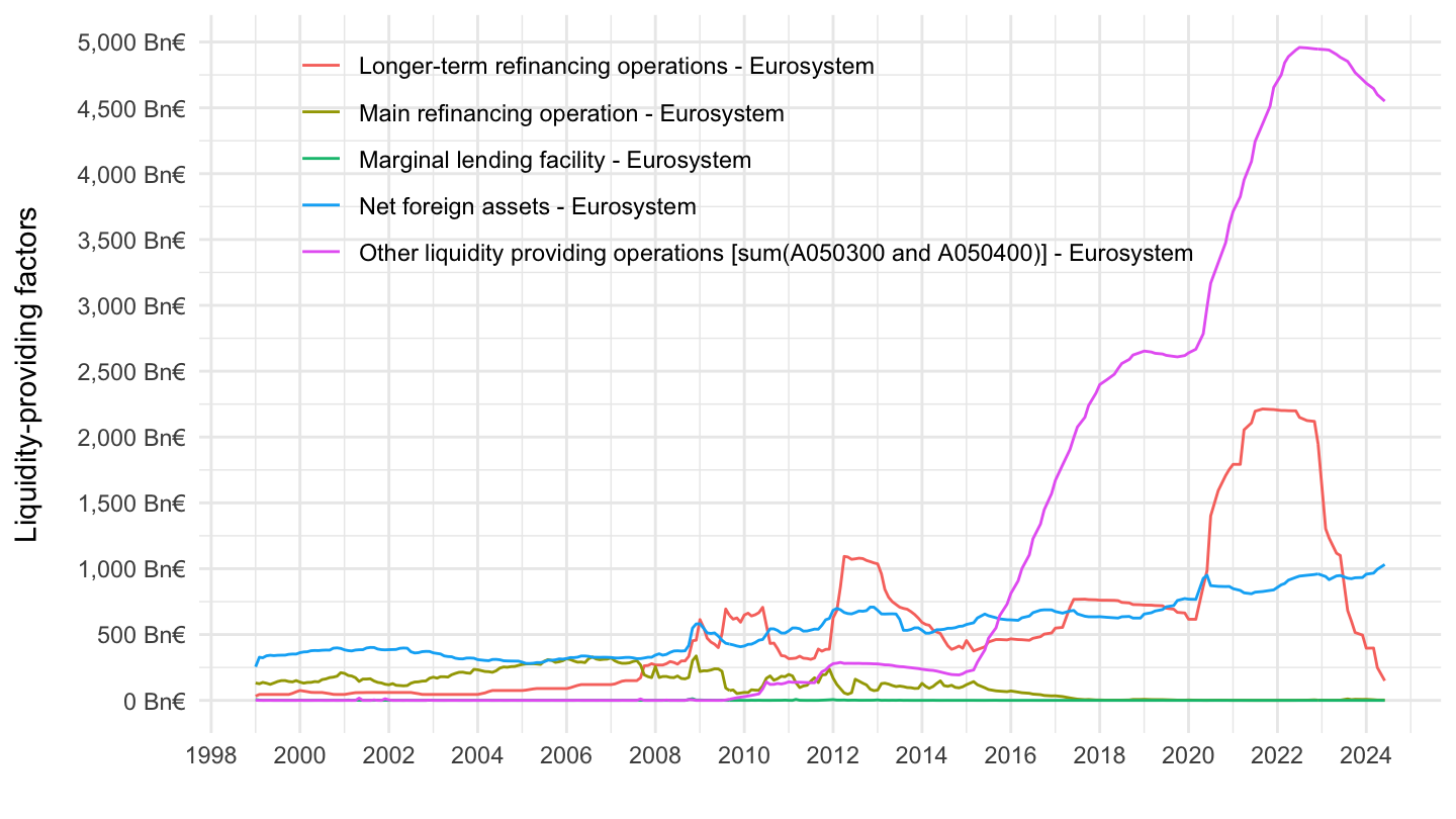
Years of GDP
Code
ILM %>%
  filter(KEY %in% c("ILM.M.U2.C.AN00001.Z5.Z0Z",
                    "ILM.M.U2.C.A050100.U2.EUR",
                    "ILM.M.U2.C.A050200.U2.EUR",
                    "ILM.M.U2.C.A050500.U2.EUR",
                    "ILM.M.U2.C.A050A00.U2.EUR")) %>%
  month_to_date %>%
  mutate(OBS_VALUE = OBS_VALUE/1000) %>%
  left_join(B1GQ %>% mutate(date = date + months(3)), by = "date") %>%
  mutate(B1GQ_i = spline(x = date, y = B1GQ, xout = date)$y) %>%
  mutate(OBS_VALUE = OBS_VALUE/B1GQ_i) %>%
  ggplot + geom_line(aes(x = date, y = OBS_VALUE, color = TITLE)) +
  ylab("Liquidity-providing factors (years of GDP)") + xlab("") + theme_minimal() +
  theme(legend.position = c(0.4, 0.8),
        legend.title = element_blank()) +
  scale_y_continuous(breaks = 0.01*seq(-5, 100, 5)) +
  scale_x_date(breaks = as.Date(paste0(seq(1940, 2100,  2), "-01-01")),
               labels = date_format("%Y"))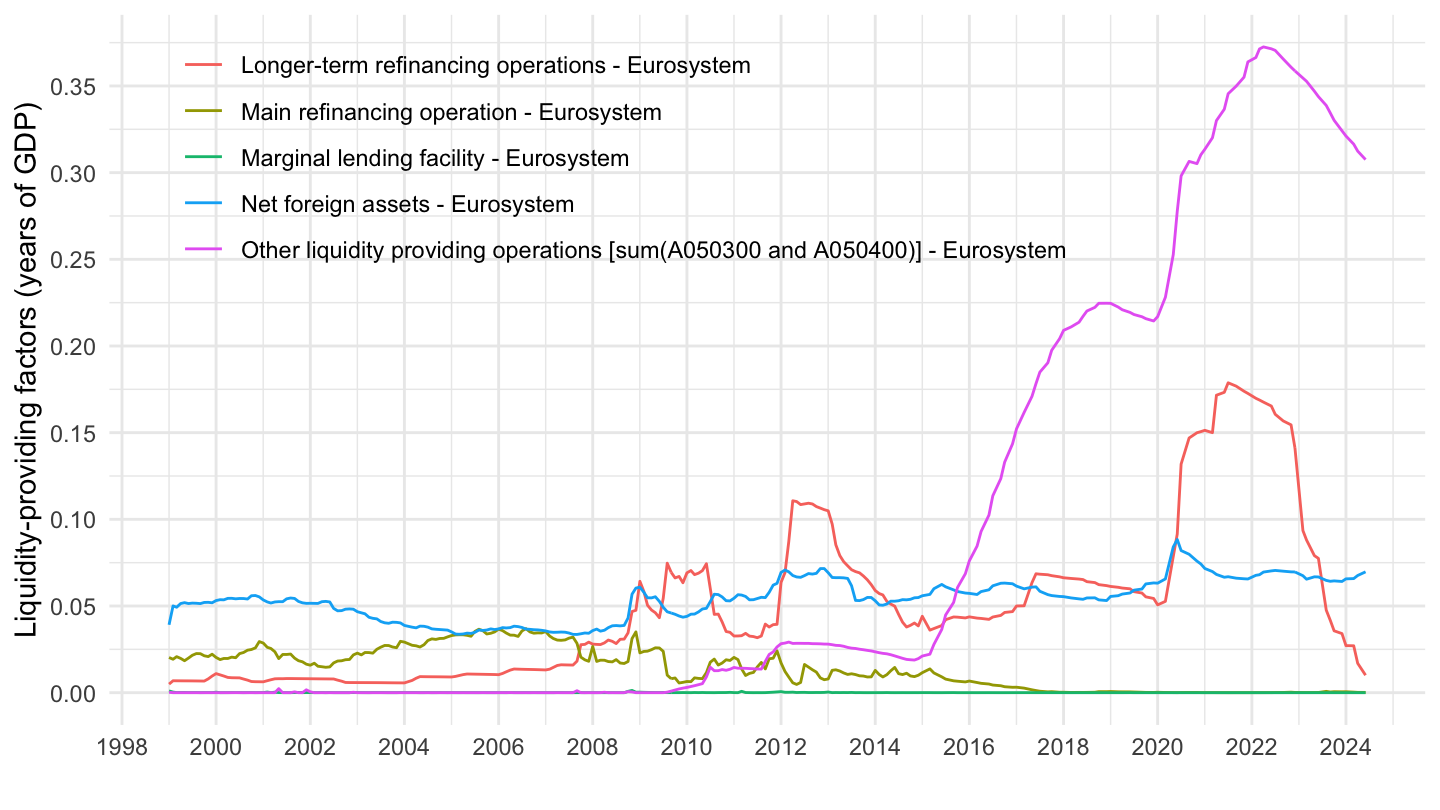
Stacked
Bn€
Code
ILM %>%
  filter(KEY %in% c("ILM.M.U2.C.AN00001.Z5.Z0Z",
                    "ILM.M.U2.C.A050100.U2.EUR",
                    "ILM.M.U2.C.A050200.U2.EUR",
                    "ILM.M.U2.C.A050500.U2.EUR",
                    "ILM.M.U2.C.A050A00.U2.EUR")) %>%
  month_to_date %>%
  mutate(OBS_VALUE = OBS_VALUE/1000) %>%
  arrange(date) %>%
  mutate(TITLE = ifelse(BS_ITEM == "A050A00", "Other liquidity providing operations", TITLE),
         TITLE = gsub(" - Eurosystem", "", TITLE)) %>%
  ggplot + geom_area(aes(x = date, y = OBS_VALUE, fill = TITLE), alpha = 0.5) +
  ylab("Liquidity-providing factors") + xlab("") + theme_minimal() +
  theme(legend.position = c(0.3, 0.75),
        legend.title = element_blank()) +
  scale_y_continuous(breaks = seq(0, 10000, 500),
                labels = dollar_format(acc = 1, pre = "", su = " Bn€")) +
  scale_x_date(breaks = as.Date(paste0(seq(1940, 2100,  2), "-01-01")),
               labels = date_format("%Y"))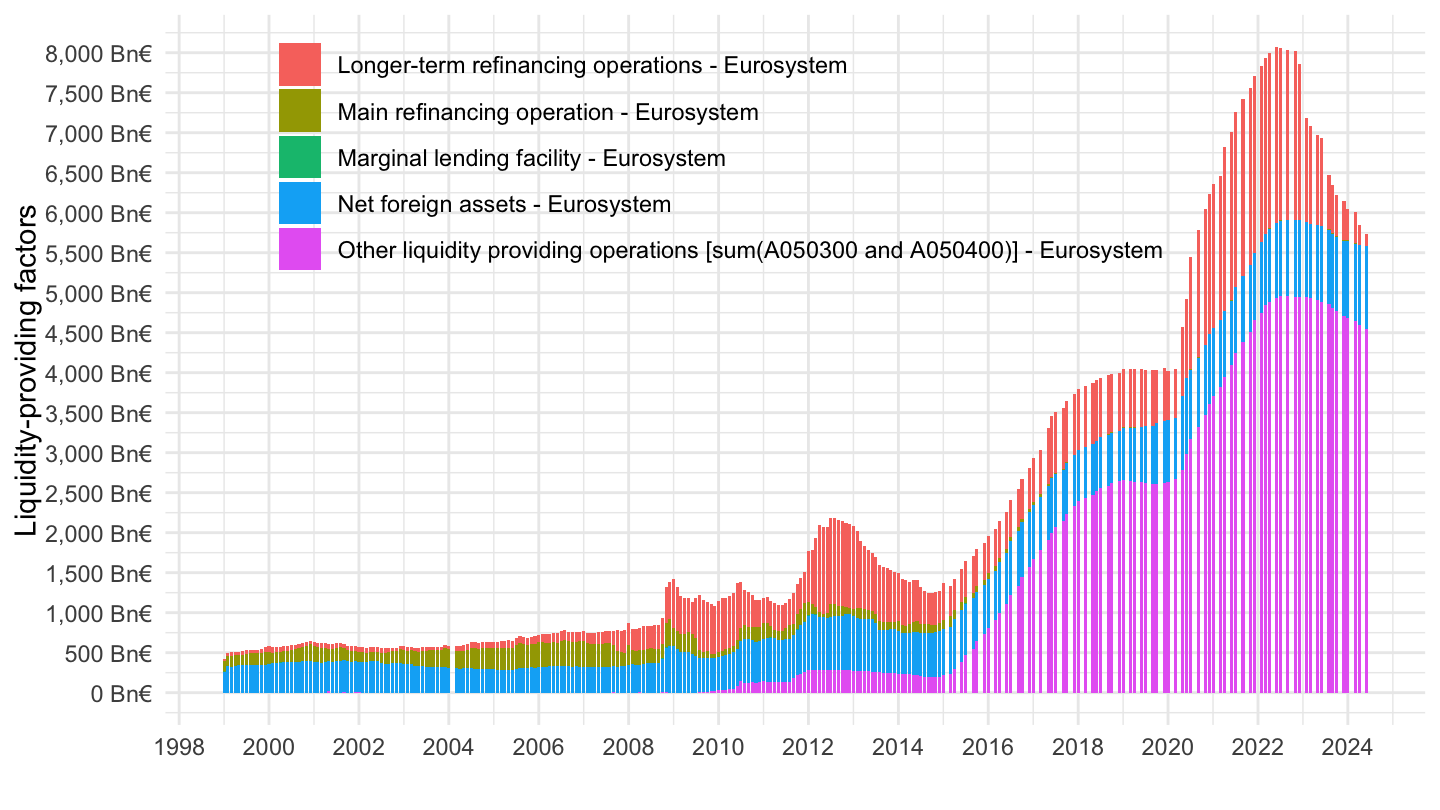
Years of GDP
Code
ILM %>%
  filter(KEY %in% c("ILM.M.U2.C.AN00001.Z5.Z0Z",
                    "ILM.M.U2.C.A050100.U2.EUR",
                    "ILM.M.U2.C.A050200.U2.EUR",
                    "ILM.M.U2.C.A050500.U2.EUR",
                    "ILM.M.U2.C.A050A00.U2.EUR")) %>%
  month_to_date %>%
  mutate(OBS_VALUE = OBS_VALUE/1000) %>%
  left_join(B1GQ %>% mutate(date = date + months(3)), by = "date") %>%
  mutate(B1GQ_i = spline(x = date, y = B1GQ, xout = date)$y) %>%
  mutate(OBS_VALUE = OBS_VALUE/B1GQ_i) %>%
  ggplot + geom_area(aes(x = date, y = OBS_VALUE, fill = TITLE), alpha = 0.5) +
  ylab("Liquidity-providing factors (years of GDP)") + xlab("") + theme_minimal() +
  theme(legend.position = c(0.4, 0.8),
        legend.title = element_blank()) +
  scale_y_continuous(breaks = 0.01*seq(-5, 100, 5)) +
  scale_x_date(breaks = as.Date(paste0(seq(1940, 2100,  2), "-01-01")),
               labels = date_format("%Y"))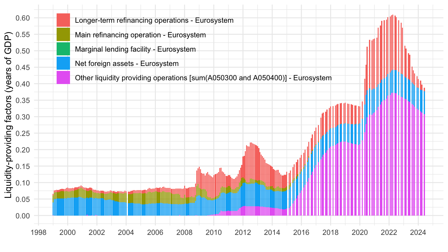
Liquidity-absorbing factors
Individual
Bn€
Code
ILM %>%
  filter(KEY %in% c("ILM.M.U2.C.L020200.U2.EUR",
                    "ILM.M.U2.C.L020300.U2.EUR",
                    "ILM.M.U2.C.L010000.Z5.EUR",
                    "ILM.M.U2.C.L050100.U2.EUR",
                    "ILM.M.U2.C.AN00002.Z5.Z0Z")) %>%
  month_to_date %>%
  mutate(OBS_VALUE = OBS_VALUE/1000) %>%
  ggplot + geom_line(aes(x = date, y = OBS_VALUE, color = TITLE)) +
  ylab("Liquidity-absorbing factors") + xlab("") + theme_minimal() +
  theme(legend.position = c(0.45, 0.8),
        legend.title = element_blank()) +
  scale_y_continuous(breaks = seq(0, 10000, 500),
                labels = dollar_format(acc = 1, pre = "", su = " Bn€")) +
  scale_x_date(breaks = as.Date(paste0(seq(1940, 2100,  2), "-01-01")),
               labels = date_format("%Y"))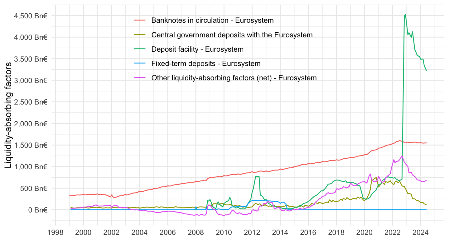
Years of GDP
Code
ILM %>%
  filter(KEY %in% c("ILM.M.U2.C.L020200.U2.EUR",
                    "ILM.M.U2.C.L020300.U2.EUR",
                    "ILM.M.U2.C.L010000.Z5.EUR",
                    "ILM.M.U2.C.L050100.U2.EUR",
                    "ILM.M.U2.C.AN00002.Z5.Z0Z")) %>%
  month_to_date %>%
  mutate(OBS_VALUE = OBS_VALUE/1000) %>%
  left_join(B1GQ %>% mutate(date = date + months(3)), by = "date") %>%
  mutate(B1GQ_i = spline(x = date, y = B1GQ, xout = date)$y) %>%
  mutate(OBS_VALUE = OBS_VALUE/B1GQ_i) %>%
  ggplot + geom_line(aes(x = date, y = OBS_VALUE, color = TITLE)) +
  ylab("Liquidity-providing factors (years of GDP)") + xlab("") + theme_minimal() +
  theme(legend.position = c(0.4, 0.8),
        legend.title = element_blank()) +
  scale_y_continuous(breaks = 0.01*seq(-5, 100, 5)) +
  scale_x_date(breaks = as.Date(paste0(seq(1940, 2100,  2), "-01-01")),
               labels = date_format("%Y"))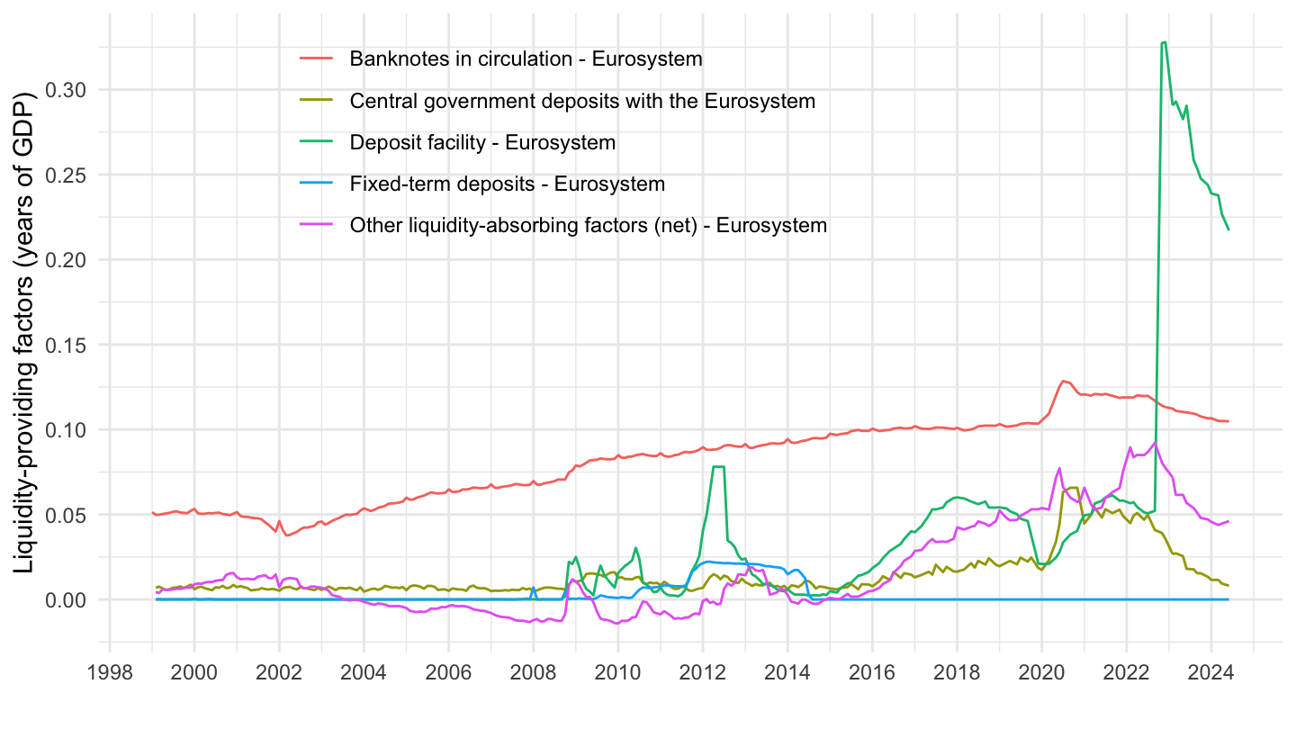
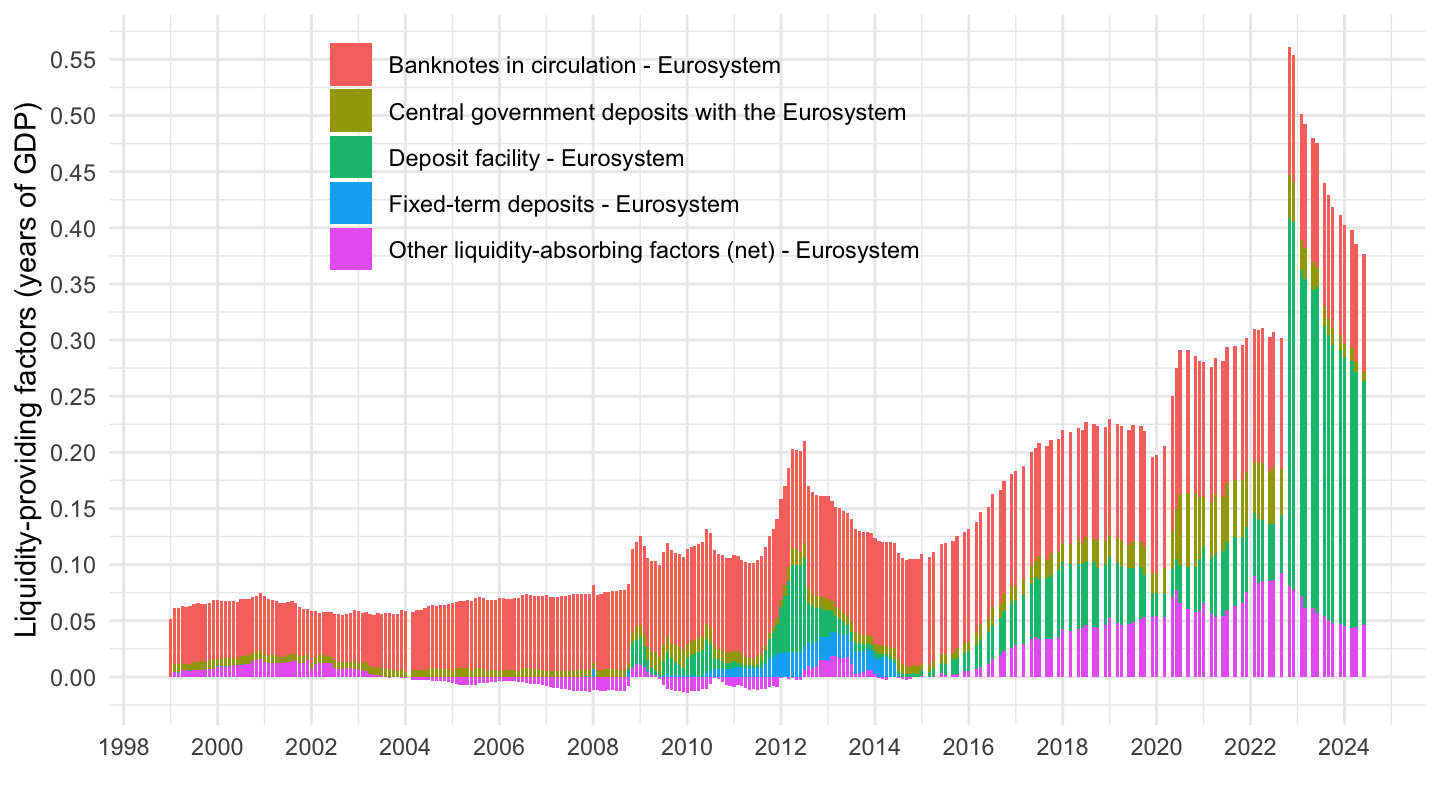
Stacked
Bn€
Code
ILM %>%
  filter(KEY %in% c("ILM.M.U2.C.L020200.U2.EUR",
                    "ILM.M.U2.C.L020300.U2.EUR",
                    "ILM.M.U2.C.L010000.Z5.EUR",
                    "ILM.M.U2.C.L050100.U2.EUR",
                    "ILM.M.U2.C.AN00002.Z5.Z0Z")) %>%
  month_to_date %>%
  mutate(OBS_VALUE = OBS_VALUE/1000) %>%
  ggplot + geom_col(aes(x = date, y = OBS_VALUE, fill = TITLE)) +
  ylab("Liquidity-absorbing factors") + xlab("") + theme_minimal() +
  theme(legend.position = c(0.45, 0.8),
        legend.title = element_blank()) +
  scale_y_continuous(breaks = seq(0, 10000, 500),
                labels = dollar_format(acc = 1, pre = "", su = " Bn€")) +
  scale_x_date(breaks = as.Date(paste0(seq(1940, 2100,  2), "-01-01")),
               labels = date_format("%Y"))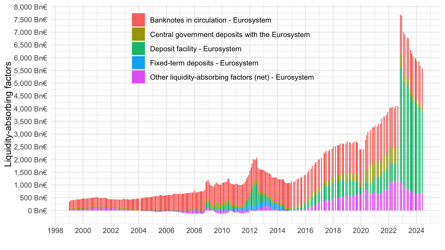
Years of GDP
Code
ILM %>%
  filter(KEY %in% c("ILM.M.U2.C.L020200.U2.EUR",
                    "ILM.M.U2.C.L020300.U2.EUR",
                    "ILM.M.U2.C.L010000.Z5.EUR",
                    "ILM.M.U2.C.L050100.U2.EUR",
                    "ILM.M.U2.C.AN00002.Z5.Z0Z")) %>%
  month_to_date %>%
  mutate(OBS_VALUE = OBS_VALUE/1000) %>%
  left_join(B1GQ %>% mutate(date = date + months(3)), by = "date") %>%
  mutate(B1GQ_i = spline(x = date, y = B1GQ, xout = date)$y) %>%
  mutate(OBS_VALUE = OBS_VALUE/B1GQ_i) %>%
  ggplot + geom_col(aes(x = date, y = OBS_VALUE, fill = TITLE)) +
  ylab("Liquidity-providing factors (years of GDP)") + xlab("") + theme_minimal() +
  theme(legend.position = c(0.4, 0.8),
        legend.title = element_blank()) +
  scale_y_continuous(breaks = 0.01*seq(-5, 100, 5)) +
  scale_x_date(breaks = as.Date(paste0(seq(1940, 2100,  2), "-01-01")),
               labels = date_format("%Y"))