Balance Sheet Items
Data - ECB
Info
Information
Data on monetary policy
| source | dataset | Title | .html | .rData |
|---|---|---|---|---|
| ecb | BSI | Balance Sheet Items | 2026-06-03 | 2026-05-22 |
| bdf | FM | NA | NA | NA |
| bdf | MIR | NA | NA | NA |
| bdf | MIR1 | NA | NA | NA |
| bis | CBPOL | Policy Rates, Daily | 2026-04-08 | 2026-06-04 |
| ecb | BSI_PUB | NA | NA | NA |
| ecb | FM | Financial market data | 2026-06-03 | 2026-06-04 |
| ecb | ILM | Internal Liquidity Management | 2026-06-03 | 2026-06-04 |
| ecb | ILM_PUB | NA | NA | NA |
| ecb | MIR | MFI Interest Rate Statistics | 2026-06-03 | 2026-06-04 |
| ecb | RAI | NA | NA | NA |
| ecb | SUP | NA | NA | NA |
| ecb | YC | NA | NA | NA |
| ecb | YC_PUB | NA | NA | NA |
| ecb | liq_daily | Daily Liquidity | 2026-06-03 | 2025-06-06 |
| eurostat | ei_mfir_m | Interest rates - monthly data | 2026-06-03 | 2026-04-26 |
| eurostat | irt_st_m | Money market interest rates - monthly data | 2026-06-03 | 2026-04-26 |
| fred | r | Interest Rates | 2026-06-04 | 2026-05-29 |
| oecd | MEI | Main Economic Indicators | 2024-04-16 | 2025-07-24 |
| oecd | MEI_FIN | Monthly Monetary and Financial Statistics (MEI) | 2024-09-15 | 2025-07-24 |
LAST_COMPILE
| LAST_COMPILE |
|---|
| 2026-07-04 |
Last
Code
BSI %>%
  group_by(TIME_PERIOD, FREQ) %>%
  summarise(Nobs = n()) %>%
  arrange(desc(TIME_PERIOD)) %>%
  head(5) %>%
print_table_conditional()| TIME_PERIOD | FREQ | Nobs |
|---|---|---|
| 2026-Q1 | Q | 2092 |
| 2026-06 | M | 1 |
| 2026-05 | M | 45 |
| 2026-03 | M | 44978 |
| 2026-02 | M | 45015 |
FREQ
Code
BSI %>%
  left_join(FREQ,  by = "FREQ") %>%
  group_by(FREQ, Freq) %>%
  summarise(Nobs = n()) %>%
  arrange(-Nobs) %>%
{if (is_html_output()) print_table(.) else .}| FREQ | Freq | Nobs |
|---|---|---|
| M | Monthly | 6743329 |
| Q | Quarterly | 1406978 |
| A | Annual | 109 |
REF_AREA
Code
BSI %>%
  left_join(REF_AREA,  by = "REF_AREA") %>%
  group_by(REF_AREA, Ref_area) %>%
  summarise(Nobs = n()) %>%
  arrange(-Nobs) %>%
  {if (is_html_output()) datatable(., filter = 'top', rownames = F) else .}
ADJUSTMENT
Code
BSI %>%
  left_join(ADJUSTMENT,  by = "ADJUSTMENT") %>%
  group_by(ADJUSTMENT, Adjustment) %>%
  summarise(Nobs = n()) %>%
  arrange(-Nobs) %>%
  {if (is_html_output()) datatable(., filter = 'top', rownames = F) else .}
BS_REP_SECTOR
Code
BSI %>%
  left_join(BS_REP_SECTOR,  by = "BS_REP_SECTOR") %>%
  group_by(BS_REP_SECTOR, Bs_rep_sector) %>%
  summarise(Nobs = n()) %>%
  arrange(-Nobs) %>%
  {if (is_html_output()) datatable(., filter = 'top', rownames = F) else .}
BS_ITEM
Code
BSI %>%
  left_join(BS_ITEM,  by = "BS_ITEM") %>%
  group_by(BS_ITEM, Bs_item) %>%
  summarise(Nobs = n()) %>%
  {if (is_html_output()) datatable(., filter = 'top', rownames = F) else .}
MATURITY_ORIG
Code
BSI %>%
  left_join(MATURITY_ORIG,  by = "MATURITY_ORIG") %>%
  group_by(MATURITY_ORIG, Maturity_orig) %>%
  summarise(Nobs = n()) %>%
  {if (is_html_output()) datatable(., filter = 'top', rownames = F) else .}
DATA_TYPE
Code
BSI %>%
  left_join(DATA_TYPE,  by = "DATA_TYPE") %>%
  group_by(DATA_TYPE, Data_type) %>%
  summarise(Nobs = n()) %>%
  {if (is_html_output()) datatable(., filter = 'top', rownames = F) else .}
COUNT_AREA
Code
BSI %>%
  left_join(COUNT_AREA,  by = "COUNT_AREA") %>%
  group_by(COUNT_AREA, Count_area) %>%
  summarise(Nobs = n()) %>%
  {if (is_html_output()) datatable(., filter = 'top', rownames = F) else .}
BS_COUNT_SECTOR
Code
BSI %>%
  left_join(BS_COUNT_SECTOR,  by = "BS_COUNT_SECTOR") %>%
  group_by(BS_COUNT_SECTOR, Bs_count_sector) %>%
  summarise(Nobs = n()) %>%
  {if (is_html_output()) datatable(., filter = 'top', rownames = F) else .}
BS_SUFFIX
Code
BSI %>%
  left_join(BS_SUFFIX,  by = "BS_SUFFIX") %>%
  group_by(BS_SUFFIX, Bs_suffix) %>%
  summarise(Nobs = n()) %>%
  {if (is_html_output()) datatable(., filter = 'top', rownames = F) else .}
COLLECTION
Code
BSI %>%
  left_join(COLLECTION,  by = "COLLECTION") %>%
  group_by(COLLECTION, Collection) %>%
  summarise(Nobs = n()) %>%
  {if (is_html_output()) datatable(., filter = 'top', rownames = F) else .}
Floating rates data
France
Households
Code
BSI %>%
  filter(REF_AREA %in% c("FR"),
         BS_COUNT_SECTOR == "2250",
         MATURITY_ORIG %in% c("KF", "HL", "KKF", "HHL")) %>%
  quarter_to_date %>%
  arrange(desc(date)) %>%
  left_join(MATURITY_ORIG, by = "MATURITY_ORIG") %>%
  mutate(OBS_VALUE = OBS_VALUE/1000) %>%
  ggplot + geom_line(aes(x = date, y = OBS_VALUE, color = Maturity_orig)) +
  ylab("") + xlab("") + theme_minimal() +
  theme(legend.title = element_blank(),
        legend.position = "bottom",
        legend.direction = "vertical") +
  scale_y_continuous(breaks = seq(0, 1000, 20)) +
  scale_x_date(breaks = as.Date(paste0(seq(1940, 2030, 2), "-01-01")),
               labels = date_format("%Y"))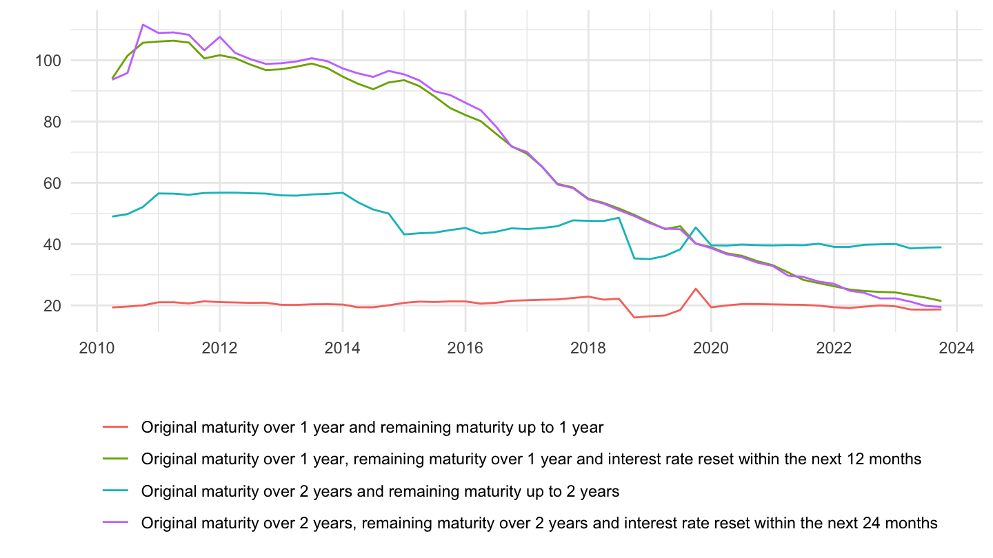
Corporations
Code
BSI %>%
  filter(REF_AREA %in% c("FR"),
         BS_COUNT_SECTOR == "2240",
         MATURITY_ORIG %in% c("KF", "HL", "KKF", "HHL")) %>%
  quarter_to_date %>%
  arrange(desc(date)) %>%
  left_join(MATURITY_ORIG, by = "MATURITY_ORIG") %>%
  mutate(OBS_VALUE = OBS_VALUE/1000) %>%
  ggplot + geom_line(aes(x = date, y = OBS_VALUE, color = Maturity_orig)) +
  ylab("") + xlab("") + theme_minimal() +
  theme(legend.title = element_blank(),
        legend.position = "bottom",
        legend.direction = "vertical") +
  scale_y_continuous(breaks = seq(0, 1000, 20)) +
  scale_x_date(breaks = as.Date(paste0(seq(1940, 2030, 2), "-01-01")),
               labels = date_format("%Y"))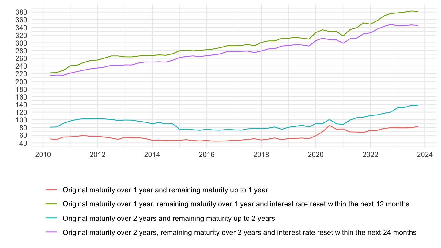
KKF - Original maturity over 1 year, remaining maturity over 1 year and interest rate reset within the next 12 months
Code
BSI %>%
  filter(MATURITY_ORIG == "KKF",
         REF_AREA %in% c("FR", "DE")) %>%
  quarter_to_date %>%
  left_join(REF_AREA, by = "REF_AREA") %>%
  left_join(BS_COUNT_SECTOR, by = "BS_COUNT_SECTOR") %>%
  mutate(OBS_VALUE = OBS_VALUE/1000) %>%
  left_join(colors, by = c("Ref_area" = "country")) %>%
  select(date, OBS_VALUE, Bs_count_sector, Ref_area, color) %>%
  ggplot + geom_line(aes(x = date, y = OBS_VALUE, color = color, linetype = Bs_count_sector)) +
  ylab("") + xlab("") + theme_minimal() +
  add_flags(4) + scale_color_identity() +
  theme(legend.position = c(0.45, 0.9),
        legend.title = element_blank()) +
  scale_y_continuous(breaks = seq(0, 1000, 20)) +
  scale_x_date(breaks = as.Date(paste0(seq(1940, 2030, 2), "-01-01")),
               labels = date_format("%Y"))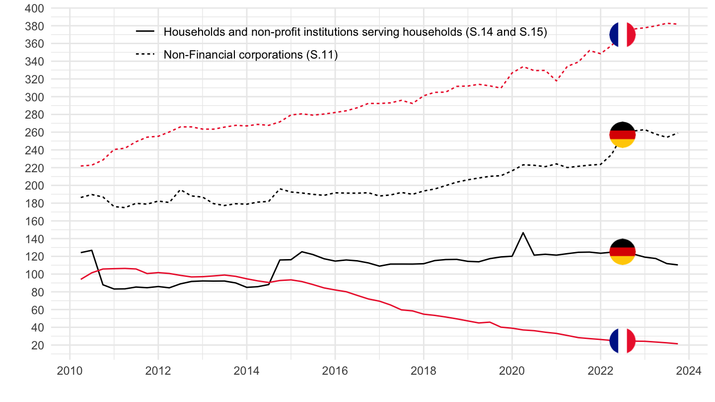
HHL - Original maturity over 2 years, remaining maturity over 2 years and interest rate reset within the next 24 months
Code
BSI %>%
  filter(MATURITY_ORIG == "HHL",
         REF_AREA %in% c("FR", "DE")) %>%
  quarter_to_date %>%
  left_join(REF_AREA, by = "REF_AREA") %>%
  left_join(BS_COUNT_SECTOR, by = "BS_COUNT_SECTOR") %>%
  mutate(OBS_VALUE = OBS_VALUE/1000) %>%
  left_join(colors, by = c("Ref_area" = "country")) %>%
  select(date, OBS_VALUE, Bs_count_sector, Ref_area, color) %>%
  ggplot + geom_line(aes(x = date, y = OBS_VALUE, color = color, linetype = Bs_count_sector)) +
  ylab("") + xlab("") + theme_minimal() +
  add_flags(4) + scale_color_identity() +
  theme(legend.position = c(0.45, 0.9),
        legend.title = element_blank()) +
  scale_y_continuous(breaks = seq(0, 1000, 20)) +
  scale_x_date(breaks = as.Date(paste0(seq(1940, 2030, 2), "-01-01")),
               labels = date_format("%Y"))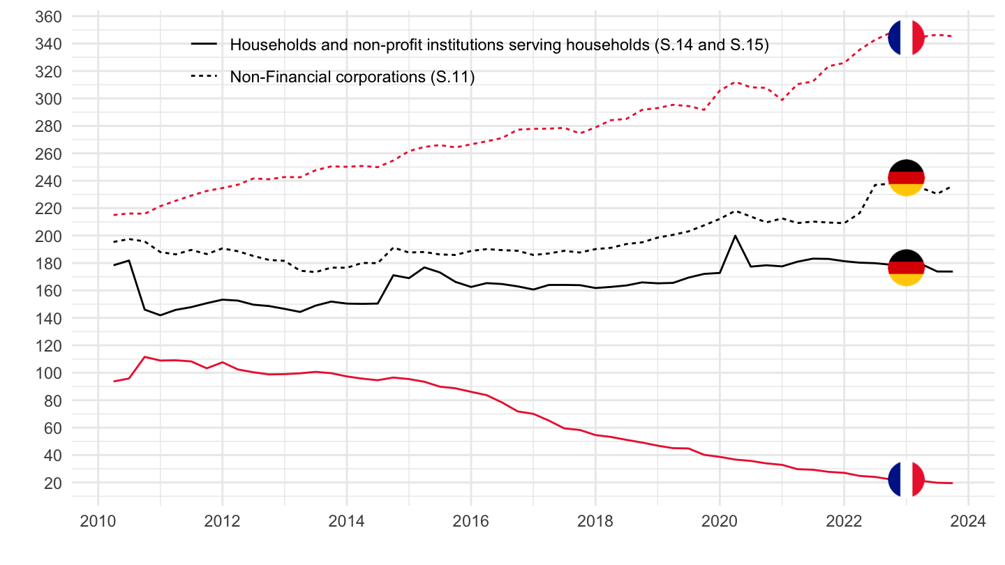
HL - Original maturity over 2 years and remaining maturity up to 2 years
Code
BSI %>%
  filter(MATURITY_ORIG == "HL",
         REF_AREA %in% c("FR", "DE")) %>%
  quarter_to_date %>%
  left_join(REF_AREA, by = "REF_AREA") %>%
  left_join(BS_COUNT_SECTOR, by = "BS_COUNT_SECTOR") %>%
  mutate(OBS_VALUE = OBS_VALUE/1000) %>%
  left_join(colors, by = c("Ref_area" = "country")) %>%
  select(date, OBS_VALUE, Bs_count_sector, Ref_area, color) %>%
  ggplot + geom_line(aes(x = date, y = OBS_VALUE, color = color, linetype = Bs_count_sector)) +
  ylab("") + xlab("") + theme_minimal() +
  add_flags(4) + scale_color_identity() +
  theme(legend.position = c(0.45, 0.9),
        legend.title = element_blank()) +
  scale_y_continuous(breaks = seq(0, 1000, 20)) +
  scale_x_date(breaks = as.Date(paste0(seq(1940, 2030, 2), "-01-01")),
               labels = date_format("%Y"))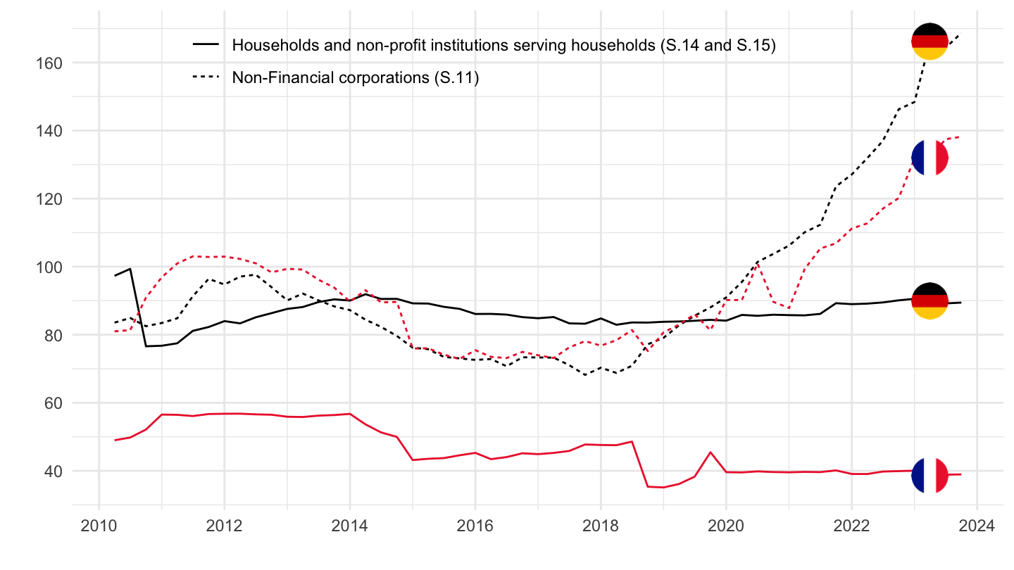
Adjusted loans
Euro area Non Financial corporations (NFCs)
France Germany, Italy
All
Code
BSI %>%
  filter(KEY %in% c("BSI.M.FR.N.A.A20T.A.I.U2.2240.Z01.A",
                    "BSI.M.IT.N.A.A20T.A.I.U2.2240.Z01.A",
                    "BSI.M.DE.N.A.A20T.A.I.U2.2240.Z01.A")) %>%
  month_to_date %>%
  left_join(REF_AREA, by = "REF_AREA") %>%
  mutate(OBS_VALUE = OBS_VALUE/100) %>%
  left_join(colors, by = c("Ref_area" = "country")) %>%
  ggplot + geom_line(aes(x = date, y = OBS_VALUE, color = color)) +
  ylab("Adjusted loans vs. € area NFCs, annual growth") + xlab("") + theme_minimal() +
  add_flags(3) + scale_color_identity() +
  theme(legend.position = c(0.45, 0.9),
        legend.title = element_blank()) +
  scale_y_continuous(breaks = 0.01*seq(-100, 90, 2),
                     labels = scales::percent_format(accuracy = 1)) +
  scale_x_date(breaks = as.Date(paste0(seq(1940, 2030, 2), "-01-01")),
               labels = date_format("%Y"))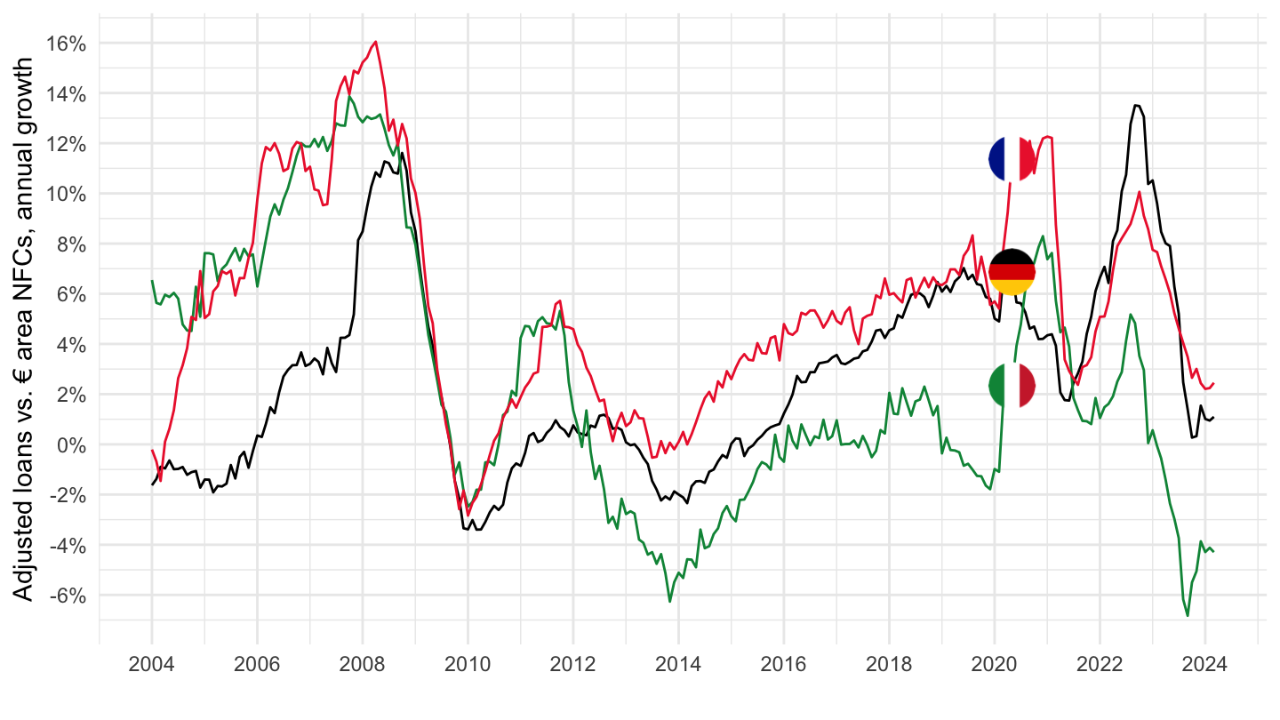
2017-
Code
BSI %>%
  filter(KEY %in% c("BSI.M.FR.N.A.A20T.A.I.U2.2240.Z01.A",
                    "BSI.M.IT.N.A.A20T.A.I.U2.2240.Z01.A",
                    "BSI.M.DE.N.A.A20T.A.I.U2.2240.Z01.A")) %>%
  month_to_date %>%
  filter(date >= as.Date("2017-01-01")) %>%
  left_join(REF_AREA, by = "REF_AREA") %>%
  mutate(OBS_VALUE = OBS_VALUE/100) %>%
  left_join(colors, by = c("Ref_area" = "country")) %>%
  ggplot + geom_line(aes(x = date, y = OBS_VALUE, color = color)) +
  ylab("Adjusted loans vs. € area NFCs, annual growth") + xlab("") + theme_minimal() +
  add_flags(3) + scale_color_identity() +
  theme(legend.position = c(0.45, 0.9),
        legend.title = element_blank()) +
  scale_y_continuous(breaks = 0.01*seq(-100, 90, 2),
                     labels = scales::percent_format(accuracy = 1)) +
  scale_x_date(breaks = as.Date(paste0(seq(1940, 2030, 1), "-01-01")),
               labels = date_format("%Y"))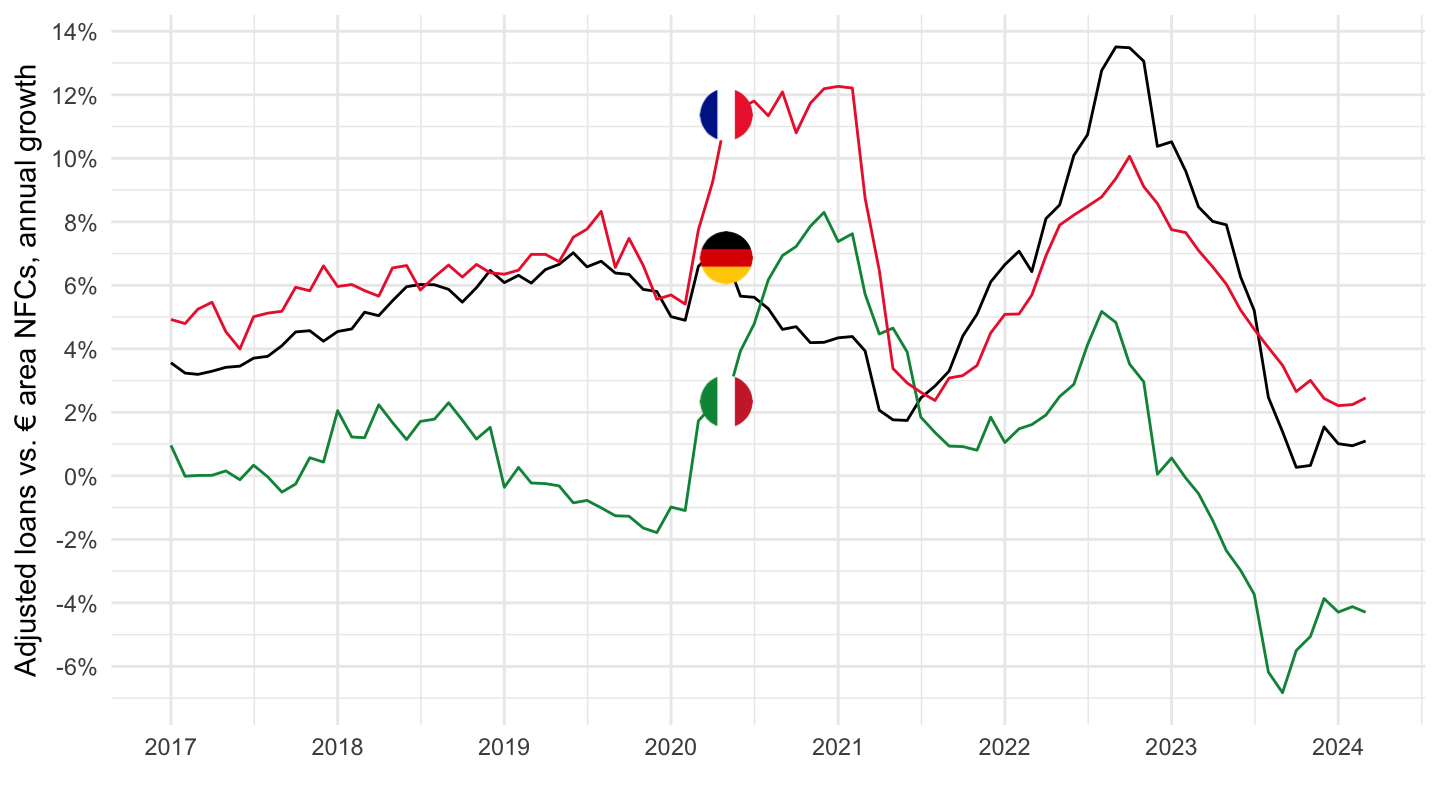
France, Germany, Italy, Euro
Table
Code
BSI %>%
  filter(FREQ == "M",
         REF_AREA == "FR",
         BS_ITEM == "A20T",
         BS_COUNT_SECTOR == "2240",
         COUNT_AREA == "U2",
         MATURITY_ORIG == "A") %>%
  select_if(~ n_distinct(.) > 1) %>%
  group_by(KEY, TITLE, TITLE_COMPL) %>%
  arrange(desc(TIME_PERIOD)) %>%
  summarise(OBS_VALUE = first(OBS_VALUE)) %>%
print_table_conditional()| KEY | TITLE | TITLE_COMPL | OBS_VALUE |
|---|---|---|---|
| BSI.M.FR.N.A.A20T.A.1.U2.2240.Z01.E | Adjusted loans to euro area NFCs granted by MFIs excluding NCB, Stocks | France, Outstanding amounts at the end of the period (stocks), MFIs excluding ESCB reporting sector - Adjusted loans, Total maturity, All currencies combined - Euro area (changing composition) counterpart, Non-Financial corporations (S.11) sector, denominated in Euro, data Neither seasonally nor working day adjusted | 1.506373e+06 |
| BSI.M.FR.N.A.A20T.A.4.U2.2240.Z01.E | Adjusted loans to euro area NFCs granted by MFIs excluding NCB, Transactions | France, Financial transactions (flows), MFIs excluding ESCB reporting sector - Adjusted loans, Total maturity, All currencies combined - Euro area (changing composition) counterpart, Non-Financial corporations (S.11) sector, denominated in Euro, data Neither seasonally nor working day adjusted | 1.195776e+04 |
| BSI.M.FR.N.A.A20T.A.I.U2.2240.Z01.A | Adjusted loans to euro area NFCs granted by MFIs excluding NCB, Annual growth rate | France, Index of Notional Stocks, MFIs excluding ESCB reporting sector - Adjusted loans, Total maturity, All currencies combined - Euro area (changing composition) counterpart, Non-Financial corporations (S.11) sector, Annual growth rate, data Neither seasonally nor working day adjusted | 3.744603e+00 |
| BSI.M.FR.Y.A.A20T.A.1.U2.2240.Z01.E | Adjusted loans to euro area NFCs granted by MFIs excluding NCB, Stocks | France, Outstanding amounts at the end of the period (stocks), MFIs excluding ESCB reporting sector - Adjusted loans, Total maturity, All currencies combined - Euro area (changing composition) counterpart, Non-Financial corporations (S.11) sector, denominated in Euro, data Working day and seasonally adjusted | 1.507705e+06 |
| BSI.M.FR.Y.A.A20T.A.4.U2.2240.Z01.E | Adjusted loans to euro area NFCs granted by MFIs excluding NCB, Transactions | France, Financial transactions (flows), MFIs excluding ESCB reporting sector - Adjusted loans, Total maturity, All currencies combined - Euro area (changing composition) counterpart, Non-Financial corporations (S.11) sector, denominated in Euro, data Working day and seasonally adjusted | 7.753000e+03 |
| BSI.M.FR.Y.A.A20T.A.I.U2.2240.Z01.A | Adjusted loans to euro area NFCs granted by MFIs excluding NCB, Annual growth rate | France, Index of Notional Stocks, MFIs excluding ESCB reporting sector - Adjusted loans, Total maturity, All currencies combined - Euro area (changing composition) counterpart, Non-Financial corporations (S.11) sector, Annual growth rate, data Working day and seasonally adjusted | 3.800192e+00 |
Outstanding amounts: manual growth
Code
BSI %>%
  filter(FREQ == "M",
         REF_AREA %in% c("FR", "DE", "U2"),
         BS_ITEM == "A20T",
         BS_COUNT_SECTOR == "2240",
         ADJUSTMENT == "Y",
         COUNT_AREA == "U2",
         MATURITY_ORIG == "A",
         DATA_TYPE == "1") %>%
  month_to_date %>%
  left_join(REF_AREA, by = "REF_AREA") %>%
  group_by(Ref_area) %>%
  arrange(date) %>%
  mutate(OBS_VALUE = OBS_VALUE/lag(OBS_VALUE, 12)-1) %>%
  mutate(Ref_area = ifelse(REF_AREA == "U2", "Europe", Ref_area)) %>%
  left_join(colors, by = c("Ref_area" = "country")) %>%
  ggplot + geom_line(aes(x = date, y = OBS_VALUE, color = color)) +
  ylab("Adjusted loans vs. € area NFCs, annual growth") + xlab("") + theme_minimal() +
  add_flags(3) + scale_color_identity() +
  theme(legend.position = c(0.45, 0.9),
        legend.title = element_blank()) +
  scale_y_continuous(breaks = 0.01*seq(-100, 90, 2),
                     labels = scales::percent_format(accuracy = 1)) +
  scale_x_date(breaks = as.Date(paste0(seq(1940, 2030, 2), "-01-01")),
               labels = date_format("%Y"))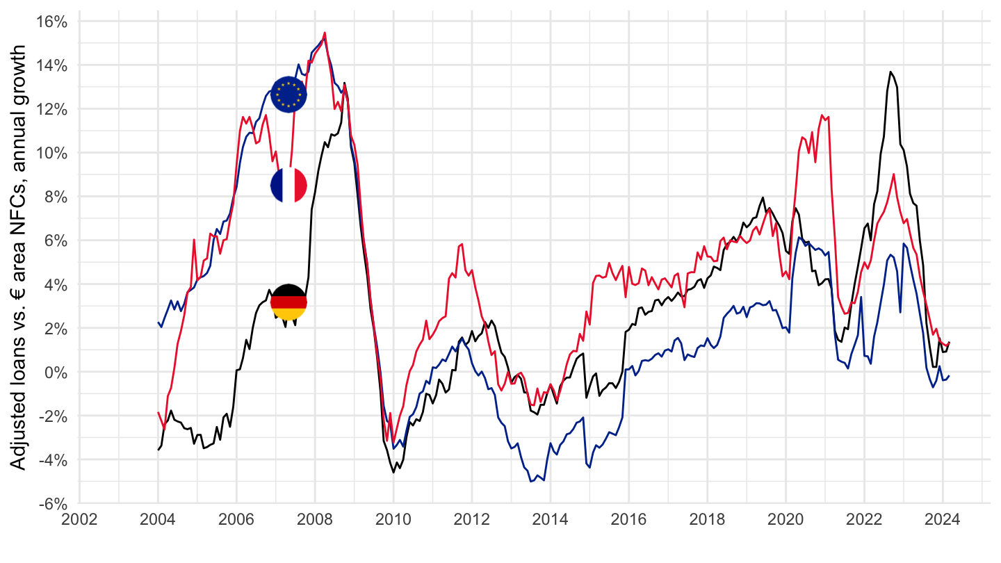
Annual growth
Code
BSI %>%
  filter(KEY %in% c("BSI.M.FR.N.A.A20T.A.I.U2.2240.Z01.A",
                    "BSI.M.IT.N.A.A20T.A.I.U2.2240.Z01.A",
                    "BSI.M.DE.N.A.A20T.A.I.U2.2240.Z01.A",
                    "BSI.M.U2.N.A.A20T.A.I.U2.2240.Z01.A")) %>%
  month_to_date %>%
  left_join(REF_AREA, by = "REF_AREA") %>%
  mutate(OBS_VALUE = OBS_VALUE/100) %>%
  mutate(Ref_area = ifelse(REF_AREA == "U2", "Europe", Ref_area)) %>%
  left_join(colors, by = c("Ref_area" = "country")) %>%
  ggplot + geom_line(aes(x = date, y = OBS_VALUE, color = color)) +
  ylab("Adjusted loans vs. € area NFCs, annual growth") + xlab("") + theme_minimal() +
  add_flags(4) + scale_color_identity() +
  theme(legend.position = c(0.45, 0.9),
        legend.title = element_blank()) +
  scale_y_continuous(breaks = 0.01*seq(-100, 90, 2),
                     labels = scales::percent_format(accuracy = 1)) +
  scale_x_date(breaks = as.Date(paste0(seq(1940, 2030, 2), "-01-01")),
               labels = date_format("%Y"))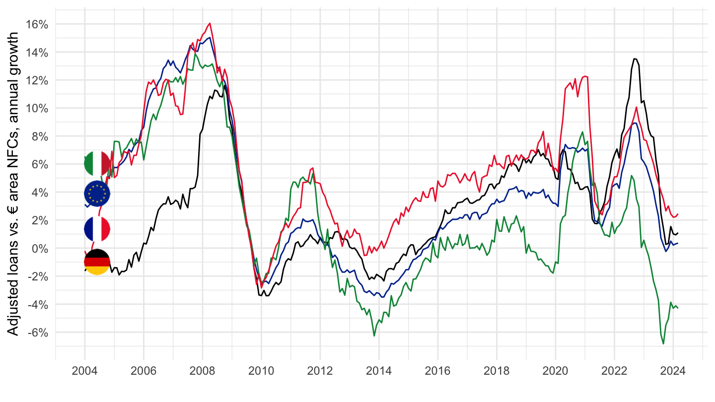
2016-
Code
BSI %>%
  filter(KEY %in% c("BSI.M.FR.N.A.A20T.A.I.U2.2240.Z01.A",
                    "BSI.M.IT.N.A.A20T.A.I.U2.2240.Z01.A",
                    "BSI.M.DE.N.A.A20T.A.I.U2.2240.Z01.A",
                    "BSI.M.U2.N.A.A20T.A.I.U2.2240.Z01.A")) %>%
  month_to_date %>%
  left_join(REF_AREA, by = "REF_AREA") %>%
  mutate(OBS_VALUE = OBS_VALUE/100) %>%
  mutate(Ref_area = ifelse(REF_AREA == "U2", "Europe", Ref_area)) %>%
  left_join(colors, by = c("Ref_area" = "country")) %>%
  filter(date >= as.Date("2016-01-01")) %>%
  ggplot + geom_line(aes(x = date, y = OBS_VALUE, color = color)) +
  ylab("Adjusted loans vs. € area NFCs, annual growth") + xlab("") + theme_minimal() +
  add_flags(4) + scale_color_identity() +
  theme(legend.position = c(0.45, 0.9),
        legend.title = element_blank()) +
  scale_y_continuous(breaks = 0.01*seq(-100, 90, 2),
                     labels = scales::percent_format(accuracy = 1)) +
  scale_x_date(breaks = as.Date(paste0(seq(1940, 2030, 1), "-01-01")),
               labels = date_format("%Y"))
2019-
Code
BSI %>%
  filter(KEY %in% c("BSI.M.FR.N.A.A20T.A.I.U2.2240.Z01.A",
                    "BSI.M.IT.N.A.A20T.A.I.U2.2240.Z01.A",
                    "BSI.M.DE.N.A.A20T.A.I.U2.2240.Z01.A")) %>%
  month_to_date %>%
  left_join(REF_AREA, by = "REF_AREA") %>%
  mutate(OBS_VALUE = OBS_VALUE/100) %>%
  filter(date >= as.Date("2021-01-01")) %>%
  left_join(colors, by = c("Ref_area" = "country")) %>%
  ggplot + geom_line(aes(x = date, y = OBS_VALUE, color = color)) +
  ylab("Adjusted loans vs. € area NFCs, annual growth") + xlab("") + theme_minimal() +
  add_flags(3) + scale_color_identity() +
  theme(legend.position = c(0.45, 0.9),
        legend.title = element_blank(),
        axis.text.x = element_text(angle = 45, vjust = 1, hjust = 1)) +
  scale_y_continuous(breaks = 0.01*seq(-100, 90, 2),
                     labels = scales::percent_format(accuracy = 1)) +
  scale_x_date(breaks = seq.Date(from = as.Date("2019-01-01"), Sys.Date(), "3 months"),
               labels = date_format("%b %Y"))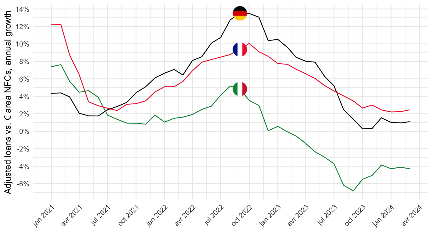
2021, all
Code
BSI %>%
  filter(FREQ == "M",
         REF_AREA %in% c("BE", "DE", "EE", "IE", "GR", "ES", "FR", "IT",
                       "LV", "LT", "LU", "MT", "NL", "AT", "PT", "SI",  "FI"),
         ADJUSTMENT == "N",
         BS_REP_SECTOR == "A",
         BS_ITEM == "A20T",
         MATURITY_ORIG == "A",
         DATA_TYPE == "I",
         COUNT_AREA == "U2",
         BS_COUNT_SECTOR == "2240") %>%
  month_to_date %>%
  left_join(REF_AREA, by = "REF_AREA") %>%
  mutate(OBS_VALUE = OBS_VALUE/100) %>%
  filter(date >= as.Date("2021-01-01")) %>%
  arrange(desc(date)) %>%
  left_join(colors, by = c("Ref_area" = "country")) %>%
  select(date, REF_AREA, color, everything()) %>%
  mutate(color = ifelse(REF_AREA == "FR", color2, color)) %>%
  ggplot + geom_line(aes(x = date, y = OBS_VALUE, color = color)) +
  ylab("Adjusted loans vs. € area NFCs, annual growth") + xlab("") + theme_minimal() +
  scale_color_identity() +
  geom_image(data = . %>%
               filter(date == as.Date("2022-09-01")) %>%
               mutate(image = paste0("../../icon/flag/round/", str_to_lower(gsub(" ", "-", Ref_area)), ".png")),
             aes(x = date, y = OBS_VALUE, image = image), asp = 1.5, size=.02) +
  theme(legend.position = c(0.45, 0.9),
        legend.title = element_blank(),
        axis.text.x = element_text(angle = 45, vjust = 1, hjust = 1)) +
  scale_y_continuous(breaks = 0.01*seq(-100, 90, 2),
                     labels = scales::percent_format(accuracy = 1)) +
  scale_x_date(breaks = seq.Date(from = as.Date("2019-01-01"), Sys.Date(), "3 months"),
               labels = date_format("%b %Y"))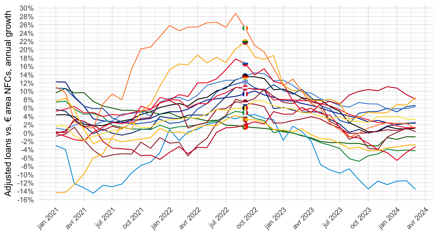
2022, all
Code
BSI %>%
  filter(FREQ == "M",
         REF_AREA %in% c("BE", "DE", "EE", "IE", "GR", "ES", "FR", "IT",
                       "LV", "LT", "LU", "MT", "NL", "AT", "PT", "SI",  "FI"),
         ADJUSTMENT == "N",
         BS_REP_SECTOR == "A",
         BS_ITEM == "A20T",
         MATURITY_ORIG == "A",
         DATA_TYPE == "I",
         COUNT_AREA == "U2",
         BS_COUNT_SECTOR == "2240") %>%
  month_to_date %>%
  left_join(REF_AREA, by = "REF_AREA") %>%
  mutate(OBS_VALUE = OBS_VALUE/100) %>%
  filter(date >= as.Date("2022-01-01")) %>%
  arrange(desc(date)) %>%
  left_join(colors, by = c("Ref_area" = "country")) %>%
  select(date, REF_AREA, color, everything()) %>%
  mutate(color = ifelse(REF_AREA == "FR", color2, color)) %>%
  ggplot + geom_line(aes(x = date, y = OBS_VALUE, color = color)) +
  ylab("Adjusted loans vs. € area NFCs, annual growth") + xlab("") + theme_minimal() +
  scale_color_identity() +
  geom_image(data = . %>%
               filter(date == as.Date("2022-09-01")) %>%
               mutate(image = paste0("../../icon/flag/round/", str_to_lower(gsub(" ", "-", Ref_area)), ".png")),
             aes(x = date, y = OBS_VALUE, image = image), asp = 1.5, size=.02) +
  theme(legend.position = c(0.45, 0.9),
        legend.title = element_blank(),
        axis.text.x = element_text(angle = 45, vjust = 1, hjust = 1)) +
  scale_y_continuous(breaks = 0.01*seq(-100, 90, 2),
                     labels = scales::percent_format(accuracy = 1)) +
  scale_x_date(breaks = seq.Date(from = as.Date("2019-01-01"), Sys.Date(), "1 month"),
               labels = date_format("%b %Y"))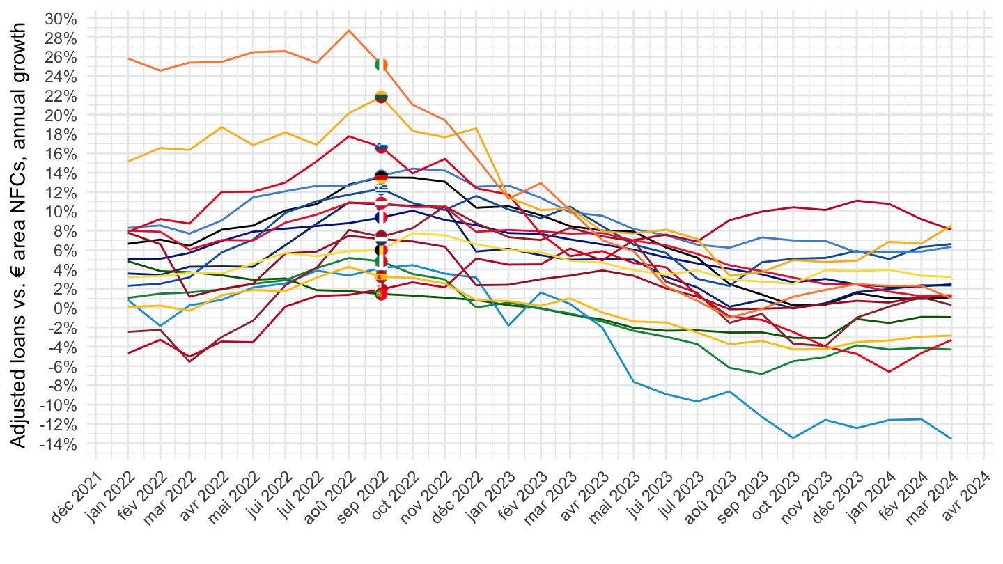
Households
France, Germany, Italy, Euro
All
Code
BSI %>%
  filter(KEY %in% c("BSI.M.FR.N.A.A20T.A.I.U2.2250.Z01.A")) %>%
  month_to_date %>%
  left_join(REF_AREA, by = "REF_AREA") %>%
  mutate(OBS_VALUE = OBS_VALUE/100) %>%
  select(date, REF_AREA, Ref_area, OBS_VALUE) %>%
  mutate(Ref_area = ifelse(REF_AREA == "U2", "Europe", Ref_area)) %>%
  left_join(colors, by = c("Ref_area" = "country")) %>%
  ggplot + geom_line(aes(x = date, y = OBS_VALUE)) +
  ylab("Adjusted loans vs. households, annual growth, France") + xlab("") + theme_minimal() +

  theme(legend.position = c(0.45, 0.9),
        legend.title = element_blank()) +
  scale_y_continuous(breaks = 0.01*seq(-100, 90, 2),
                     labels = scales::percent_format(accuracy = 1)) +
  scale_x_date(breaks = as.Date(paste0(seq(1940, 2030, 2), "-01-01")),
               labels = date_format("%Y"))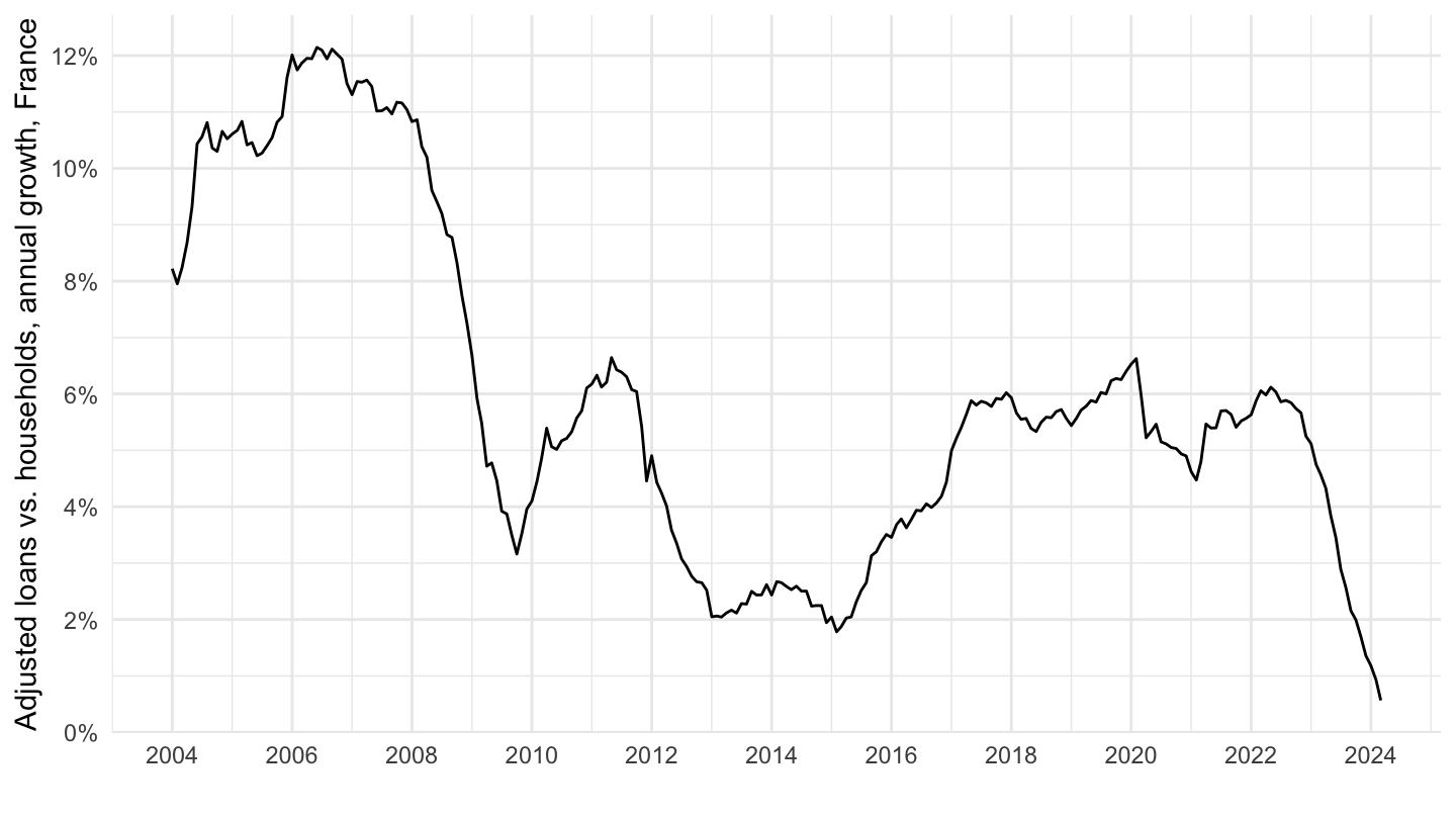
France, Germany, Italy, Euro
All
Code
data <- BSI %>%
  filter(KEY %in% c("BSI.M.FR.N.A.A20T.A.I.U2.2250.Z01.A",
                    "BSI.M.IT.N.A.A20T.A.I.U2.2250.Z01.A",
                    "BSI.M.DE.N.A.A20T.A.I.U2.2250.Z01.A",
                    "BSI.M.U2.N.A.A20T.A.I.U2.2250.Z01.A")) %>%
  month_to_date %>%
  left_join(REF_AREA, by = "REF_AREA") %>%
  mutate(OBS_VALUE = OBS_VALUE/100) %>%
  select(date, REF_AREA, Ref_area, OBS_VALUE)
write_excel_csv(data, file = "BSI_alter_eco.csv")
BSI %>%
  filter(KEY %in% c("BSI.M.FR.N.A.A20T.A.I.U2.2250.Z01.A",
                    "BSI.M.IT.N.A.A20T.A.I.U2.2250.Z01.A",
                    "BSI.M.DE.N.A.A20T.A.I.U2.2250.Z01.A",
                    "BSI.M.U2.N.A.A20T.A.I.U2.2250.Z01.A")) %>%
  month_to_date %>%
  left_join(REF_AREA, by = "REF_AREA") %>%
  mutate(OBS_VALUE = OBS_VALUE/100) %>%
  select(date, REF_AREA, Ref_area, OBS_VALUE) %>%
  mutate(Ref_area = ifelse(REF_AREA == "U2", "Europe", Ref_area)) %>%
  left_join(colors, by = c("Ref_area" = "country")) %>%
  ggplot + geom_line(aes(x = date, y = OBS_VALUE, color = color)) +
  ylab("Adjusted loans vs. € area households, annual growth") + xlab("") + theme_minimal() +
  add_flags(4) + scale_color_identity() +
  theme(legend.position = c(0.45, 0.9),
        legend.title = element_blank()) +
  scale_y_continuous(breaks = 0.01*seq(-100, 90, 2),
                     labels = scales::percent_format(accuracy = 1)) +
  scale_x_date(breaks = as.Date(paste0(seq(1940, 2030, 2), "-01-01")),
               labels = date_format("%Y"))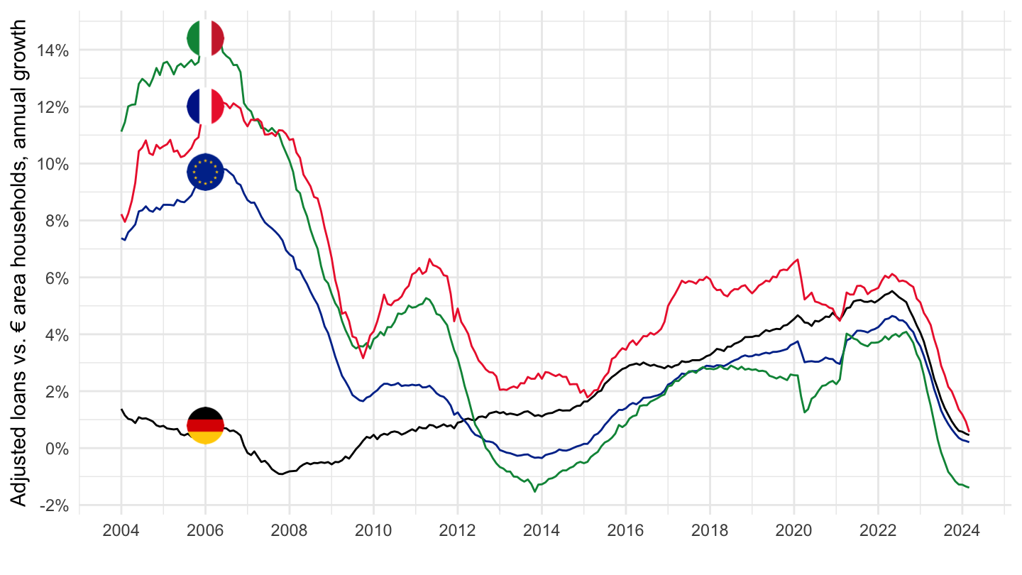
2016-
Code
BSI %>%
  filter(KEY %in% c("BSI.M.FR.N.A.A20T.A.I.U2.2240.Z01.A",
                    "BSI.M.IT.N.A.A20T.A.I.U2.2240.Z01.A",
                    "BSI.M.DE.N.A.A20T.A.I.U2.2240.Z01.A",
                    "BSI.M.U2.N.A.A20T.A.I.U2.2240.Z01.A")) %>%
  month_to_date %>%
  left_join(REF_AREA, by = "REF_AREA") %>%
  mutate(OBS_VALUE = OBS_VALUE/100) %>%
  mutate(Ref_area = ifelse(REF_AREA == "U2", "Europe", Ref_area)) %>%
  left_join(colors, by = c("Ref_area" = "country")) %>%
  filter(date >= as.Date("2016-01-01")) %>%
  ggplot + geom_line(aes(x = date, y = OBS_VALUE, color = color)) +
  ylab("Adjusted loans vs. € area households, annual growth") + xlab("") + theme_minimal() +
  add_flags(4) + scale_color_identity() +
  theme(legend.position = c(0.45, 0.9),
        legend.title = element_blank()) +
  scale_y_continuous(breaks = 0.01*seq(-100, 90, 2),
                     labels = scales::percent_format(accuracy = 1)) +
  scale_x_date(breaks = as.Date(paste0(seq(1940, 2030, 1), "-01-01")),
               labels = date_format("%Y"))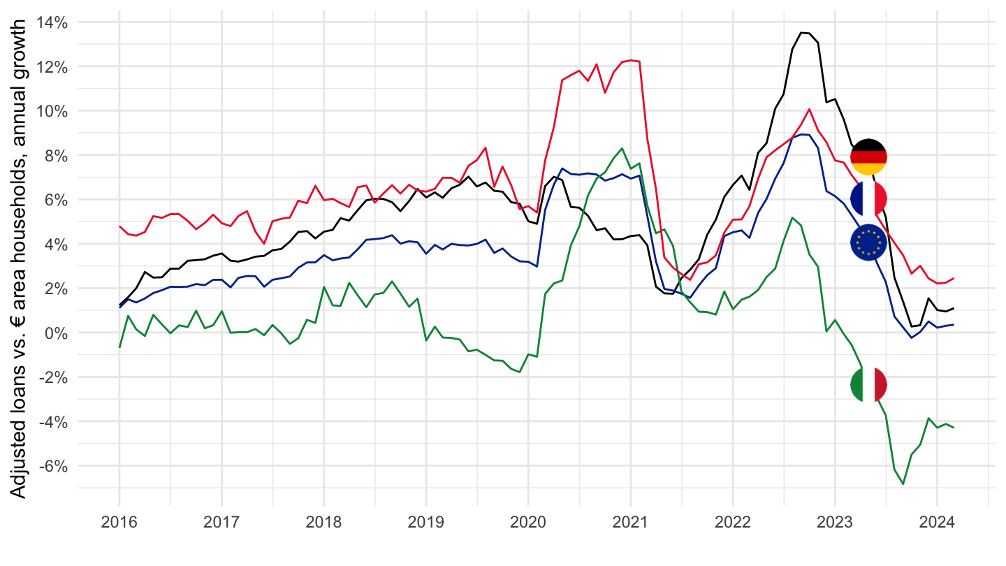
All
Code
BSI %>%
  filter(KEY %in% c("BSI.M.FR.N.A.A20T.A.I.U2.2250.Z01.A",
                    "BSI.M.IT.N.A.A20T.A.I.U2.2250.Z01.A",
                    "BSI.M.DE.N.A.A20T.A.I.U2.2250.Z01.A")) %>%
  month_to_date %>%
  left_join(REF_AREA, by = "REF_AREA") %>%
  mutate(OBS_VALUE = OBS_VALUE/100) %>%
  left_join(colors, by = c("Ref_area" = "country")) %>%
  ggplot + geom_line(aes(x = date, y = OBS_VALUE, color = color)) +
  ylab("Adjusted loans vs. households, annual growth") + xlab("") + theme_minimal() +
  add_flags(3) + scale_color_identity() +
  theme(legend.position = c(0.45, 0.9),
        legend.title = element_blank()) +
  scale_y_continuous(breaks = 0.01*seq(-100, 90, 2),
                     labels = scales::percent_format(accuracy = 1)) +
  scale_x_date(breaks = as.Date(paste0(seq(1940, 2030, 2), "-01-01")),
               labels = date_format("%Y"))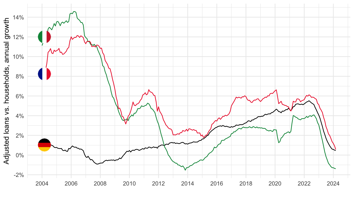
2021, all
Code
BSI %>%
  filter(FREQ == "M",
         REF_AREA %in% c("BE", "DE", "EE", "IE", "GR", "ES", "FR", "IT",
                       "LV", "LT", "LU", "MT", "NL", "AT", "PT", "SI",  "FI"),
         ADJUSTMENT == "N",
         BS_REP_SECTOR == "A",
         BS_ITEM == "A20T",
         MATURITY_ORIG == "A",
         DATA_TYPE == "I",
         COUNT_AREA == "U2",
         BS_COUNT_SECTOR == "2250") %>%
  month_to_date %>%
  left_join(REF_AREA, by = "REF_AREA") %>%
  mutate(OBS_VALUE = OBS_VALUE/100) %>%
  filter(date >= as.Date("2021-01-01")) %>%
  arrange(desc(date)) %>%
  left_join(colors, by = c("Ref_area" = "country")) %>%
  select(date, REF_AREA, color, everything()) %>%
  mutate(color = ifelse(REF_AREA == "FR", color2, color)) %>%
  ggplot + geom_line(aes(x = date, y = OBS_VALUE, color = color)) +
  ylab("Adjusted loans vs. households, annual growth") + xlab("") + theme_minimal() +
  scale_color_identity() +
  geom_image(data = . %>%
               filter(date == as.Date("2023-02-01")) %>%
               mutate(image = paste0("../../icon/flag/round/", str_to_lower(gsub(" ", "-", Ref_area)), ".png")),
             aes(x = date, y = OBS_VALUE, image = image), asp = 1.5, size = .02) +
  theme(legend.position = c(0.45, 0.9),
        legend.title = element_blank(),
        axis.text.x = element_text(angle = 45, vjust = 1, hjust = 1)) +
  scale_y_continuous(breaks = 0.01*seq(-100, 90, 2),
                     labels = scales::percent_format(accuracy = 1)) +
  scale_x_date(breaks = seq.Date(from = as.Date("2019-01-01"), Sys.Date(), "3 months"),
               labels = date_format("%b %Y"))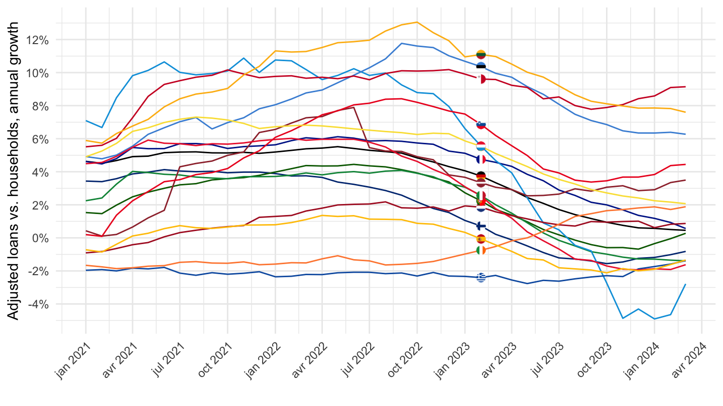
2022, all
Code
BSI %>%
  filter(FREQ == "M",
         REF_AREA %in% c("BE", "DE", "EE", "IE", "GR", "ES", "FR", "IT",
                       "LV", "LT", "LU", "MT", "NL", "AT", "PT", "SI",  "FI"),
         ADJUSTMENT == "N",
         BS_REP_SECTOR == "A",
         BS_ITEM == "A20T",
         MATURITY_ORIG == "A",
         DATA_TYPE == "I",
         COUNT_AREA == "U2",
         BS_COUNT_SECTOR == "2250") %>%
  month_to_date %>%
  left_join(REF_AREA, by = "REF_AREA") %>%
  mutate(OBS_VALUE = OBS_VALUE/100) %>%
  filter(date >= as.Date("2022-01-01")) %>%
  arrange(desc(date)) %>%
  left_join(colors, by = c("Ref_area" = "country")) %>%
  select(date, REF_AREA, color, everything()) %>%
  mutate(color = ifelse(REF_AREA == "FR", color2, color)) %>%
  ggplot + geom_line(aes(x = date, y = OBS_VALUE, color = color)) +
  ylab("Adjusted loans vs. households, annual growth") + xlab("") + theme_minimal() +
  scale_color_identity() +
  geom_image(data = . %>%
               filter(date == as.Date("2023-02-01")) %>%
               mutate(image = paste0("../../icon/flag/round/", str_to_lower(gsub(" ", "-", Ref_area)), ".png")),
             aes(x = date, y = OBS_VALUE, image = image), asp = 1.5, size = .02) +
  theme(legend.position = c(0.45, 0.9),
        legend.title = element_blank(),
        axis.text.x = element_text(angle = 45, vjust = 1, hjust = 1)) +
  scale_y_continuous(breaks = 0.01*seq(-100, 90, 2),
                     labels = scales::percent_format(accuracy = 1)) +
  scale_x_date(breaks = seq.Date(from = as.Date("2019-01-01"), Sys.Date(), "1 month"),
               labels = date_format("%b %Y"))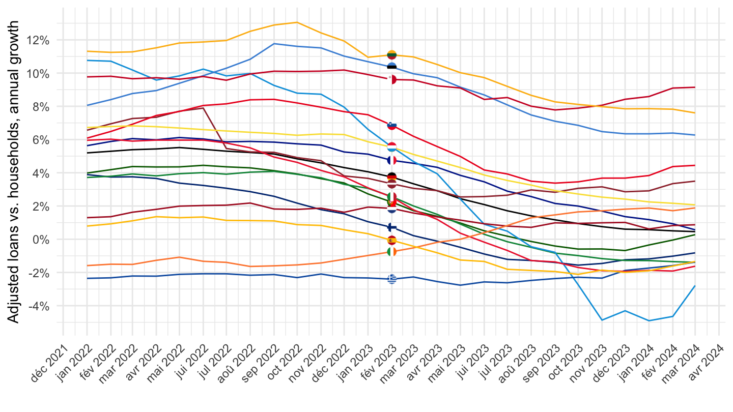
Monetary aggregates
M1
Code
BSI %>%
  filter(KEY %in% c("BSI.M.U2.Y.V.M10.X.1.U2.2300.Z01.E",
                    "BSI.M.U2.N.V.M10.X.1.U2.2300.Z01.E")) %>%
  left_join(BS_ITEM,  by = "BS_ITEM") %>%
  month_to_date %>%
  arrange(desc(date)) %>%
  ggplot + geom_line(aes(x = date, y = OBS_VALUE/10^3, color = KEY)) +
  xlab("") + ylab("") + theme_minimal() +
  scale_x_date(breaks = as.Date(paste0(seq(1940, 2030, 5), "-01-01")),
               labels = date_format("%Y")) +
  theme(legend.position = c(0.25, 0.9),
        legend.title = element_blank()) +
  scale_y_continuous(breaks = 1000*seq(-100, 90, 1),
                     labels = scales::dollar_format(acc = 1, su = " Bn€", pre = "")) +
  geom_hline(yintercept = 0, linetype = "dashed")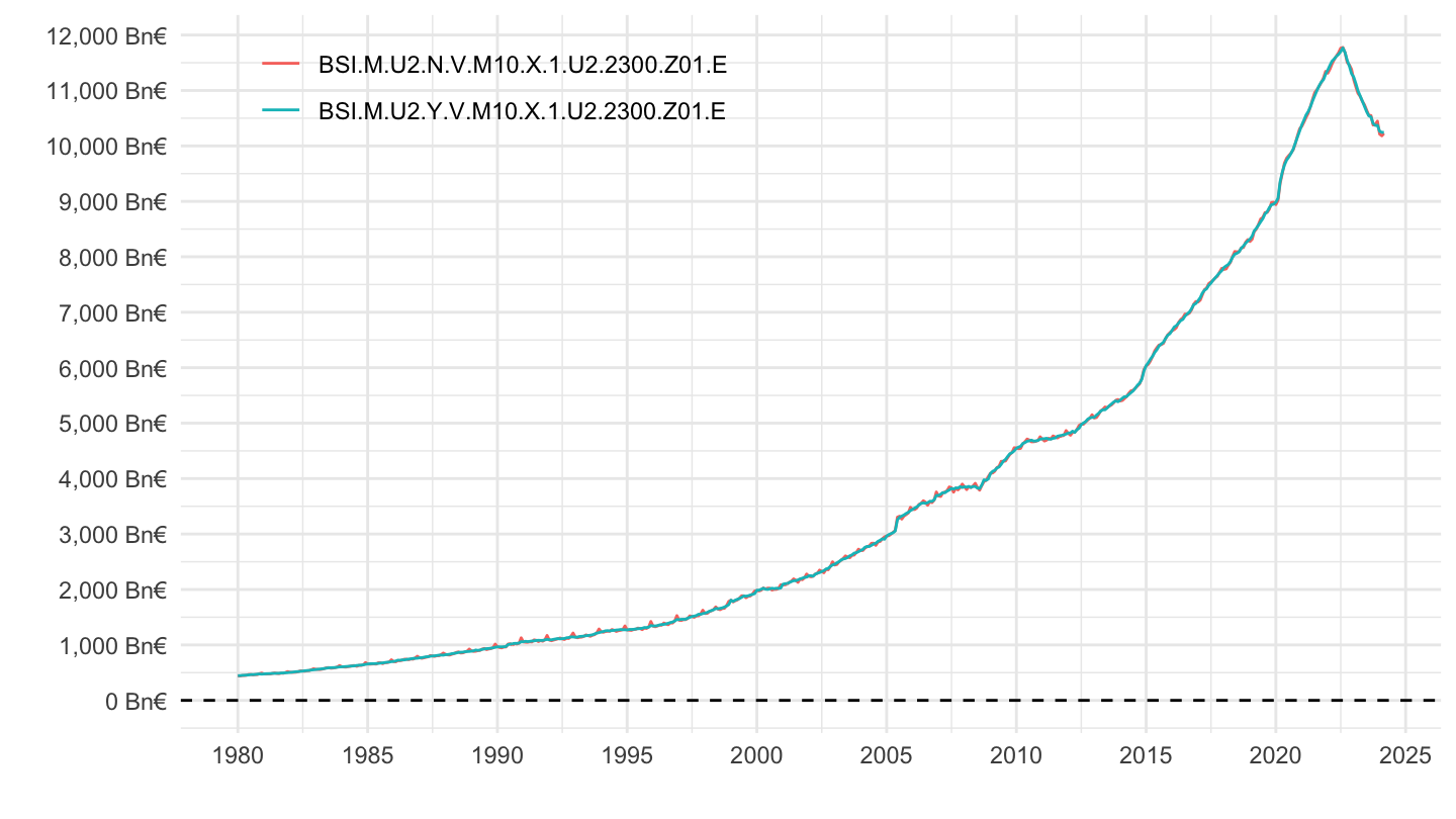
M1, M2, M3
Niveau
Code
BSI %>%
  filter(BS_ITEM %in% c("M10", "M20", "M30"),
         BS_SUFFIX == "E",
         FREQ == "M",
         ADJUSTMENT == "N",
         COLLECTION == "E",
         DATA_TYPE == "1") %>%
  left_join(BS_ITEM,  by = "BS_ITEM") %>%
  month_to_date %>%
  arrange(desc(date)) %>%
  ggplot + geom_line(aes(x = date, y = OBS_VALUE/10^3, color = Bs_item)) +
  xlab("") + ylab("") + theme_minimal() +
  scale_x_date(breaks = as.Date(paste0(seq(1940, 2030, 5), "-01-01")),
               labels = date_format("%Y")) +
  theme(legend.position = c(0.25, 0.9),
        legend.title = element_blank()) +
  scale_y_continuous(breaks = 1000*seq(-100, 90, 1),
                     labels = scales::dollar_format(acc = 1, su = " Bn€", pre = "")) +
  geom_hline(yintercept = 0, linetype = "dashed")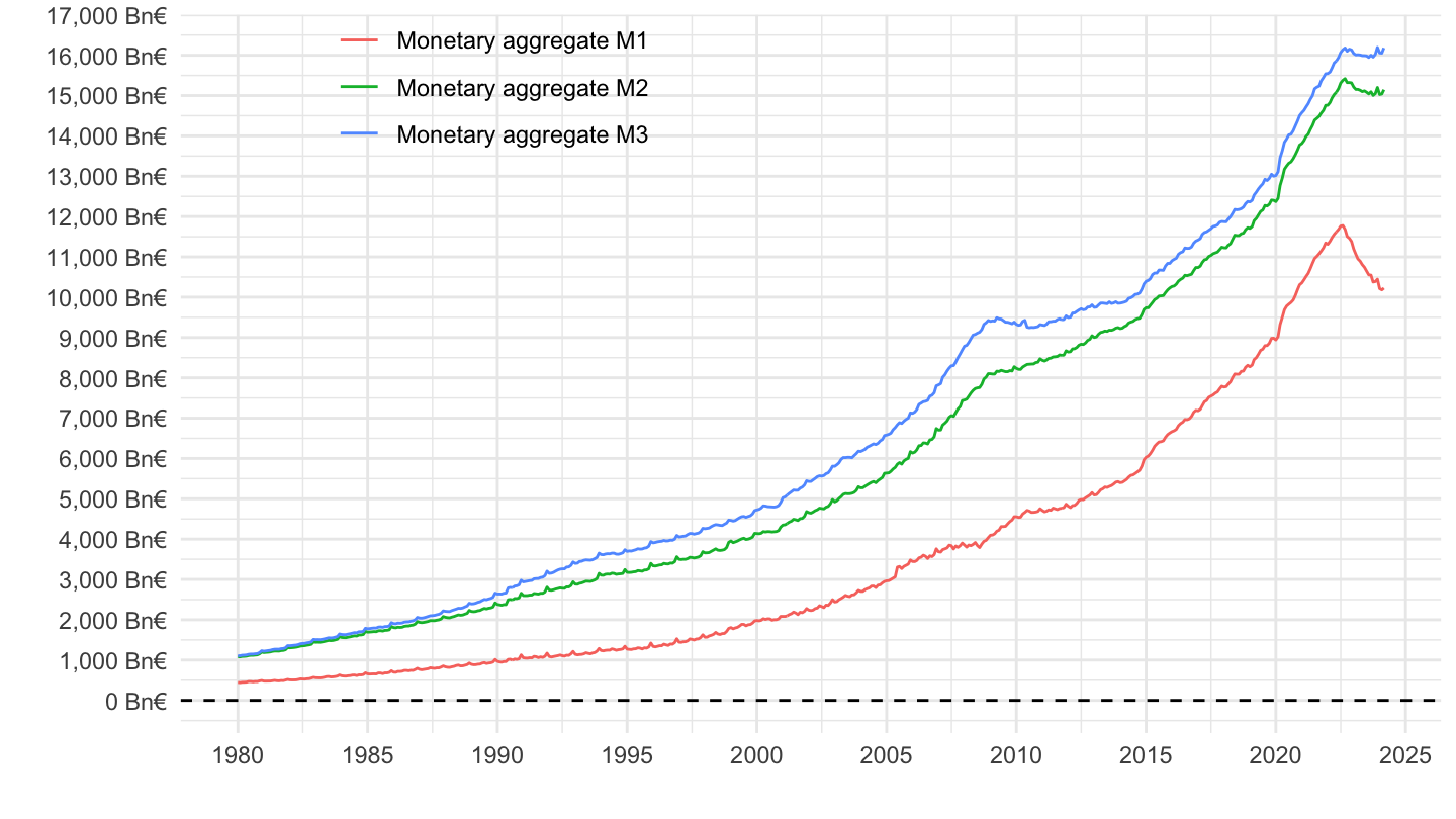
Croissance
Code
BSI %>%
  filter(BS_ITEM %in% c("M10", "M20", "M30"),
         BS_SUFFIX == "A",
         FREQ == "M") %>%
  left_join(BS_ITEM,  by = "BS_ITEM") %>%
  month_to_date %>%
  ggplot + geom_line(aes(x = date, y = OBS_VALUE/100, color = Bs_item)) +
  xlab("") + ylab("") + theme_minimal() +
  scale_x_date(breaks = as.Date(paste0(seq(1940, 2030, 5), "-01-01")),
               labels = date_format("%Y")) +
  theme(legend.position = c(0.25, 0.9),
        legend.title = element_blank()) +
  scale_y_continuous(breaks = 0.01*seq(-100, 90, 2),
                     labels = scales::percent_format(accuracy = 1)) +
  geom_hline(yintercept = 0, linetype = "dashed")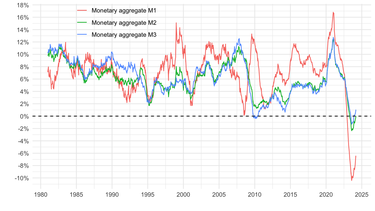
M1
M1 = overnights deposits + currency in circulation.
Level
Code
BSI %>%
  filter(BS_ITEM %in% c("L10", "L21", "M10"),
         BS_COUNT_SECTOR == "2300",
         BS_SUFFIX == "E",
         FREQ == "M",
         ADJUSTMENT == "N",
         COLLECTION == "E",
         DATA_TYPE == "1",
         BS_REP_SECTOR == "V",
         REF_AREA == "U2") %>%
  left_join(BS_ITEM,  by = "BS_ITEM") %>%
  month_to_date %>%
  arrange(desc(date)) %>%
  group_by(date) %>%
  filter(n() == 3) %>%
  mutate(Bs_item = factor(Bs_item, levels = c("Monetary aggregate M1", "Overnight deposits", "Currency in circulation"))) %>%
  ggplot + geom_line(aes(x = date, y = OBS_VALUE/10^3, color = Bs_item)) +
  xlab("") + ylab("") + theme_minimal() +
  scale_x_date(breaks = as.Date(paste0(seq(1940, 2030, 2), "-01-01")),
               labels = date_format("%Y")) +
  theme(legend.position = c(0.25, 0.9),
        legend.title = element_blank()) +
  scale_y_continuous(breaks = 1000*seq(-100, 90, 1),
                     labels = scales::dollar_format(acc = 1, su = " Bn€", pre = "")) +
  geom_hline(yintercept = 0, linetype = "dashed")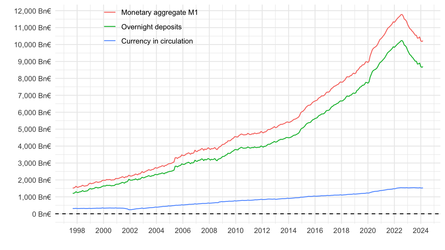
Growth
All
Code
BSI %>%
  filter(BS_ITEM %in% c("L10", "L21", "M10"),
         BS_COUNT_SECTOR == "2300",
         BS_SUFFIX == "A",
         FREQ == "M",
         BS_REP_SECTOR == "V",
         REF_AREA == "U2",
         ADJUSTMENT == "N") %>%
  left_join(BS_ITEM,  by = "BS_ITEM") %>%
  month_to_date %>%
  arrange(desc(date)) %>%
  ggplot + geom_line(aes(x = date, y = OBS_VALUE/100, color = Bs_item)) +
  xlab("") + ylab("") + theme_minimal() +
  scale_x_date(breaks = as.Date(paste0(seq(1940, 2030, 2), "-01-01")),
               labels = date_format("%b %Y")) +
  theme(legend.position = c(0.25, 0.9),
        legend.title = element_blank()) +
  scale_y_continuous(breaks = 0.01*seq(-100, 90, 2),
                     labels = scales::percent_format(accuracy = 1)) +
  geom_hline(yintercept = 0, linetype = "dashed")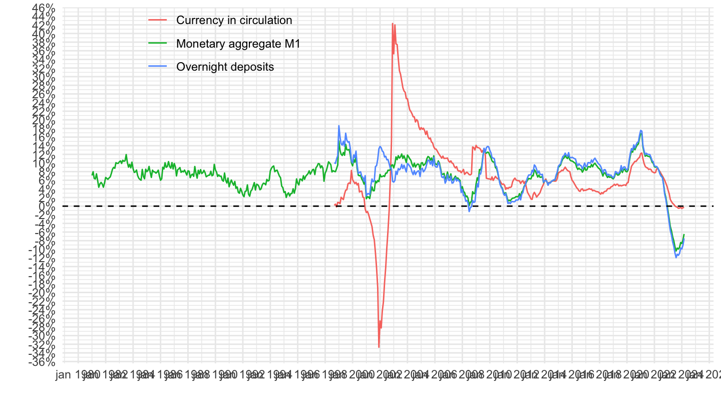
2005-
Code
BSI %>%
  filter(BS_ITEM %in% c("L10", "L21", "M10"),
         BS_COUNT_SECTOR == "2300",
         BS_SUFFIX == "A",
         FREQ == "M",
         BS_REP_SECTOR == "V",
         REF_AREA == "U2",
         ADJUSTMENT == "N") %>%
  left_join(BS_ITEM,  by = "BS_ITEM") %>%
  month_to_date %>%
  arrange(desc(date)) %>%
  filter(date >= as.Date("2005-01-01")) %>%
  ggplot + geom_line(aes(x = date, y = OBS_VALUE/100, color = Bs_item)) +
  xlab("") + ylab("") + theme_minimal() +
  scale_x_date(breaks = as.Date(paste0(seq(1940, 2030, 2), "-01-01")),
               labels = date_format("%Y")) +
  theme(legend.position = c(0.25, 0.2),
        legend.title = element_blank()) +
  scale_y_continuous(breaks = 0.01*seq(-100, 90, 2),
                     labels = scales::percent_format(accuracy = 1)) +
  geom_hline(yintercept = 0, linetype = "dashed")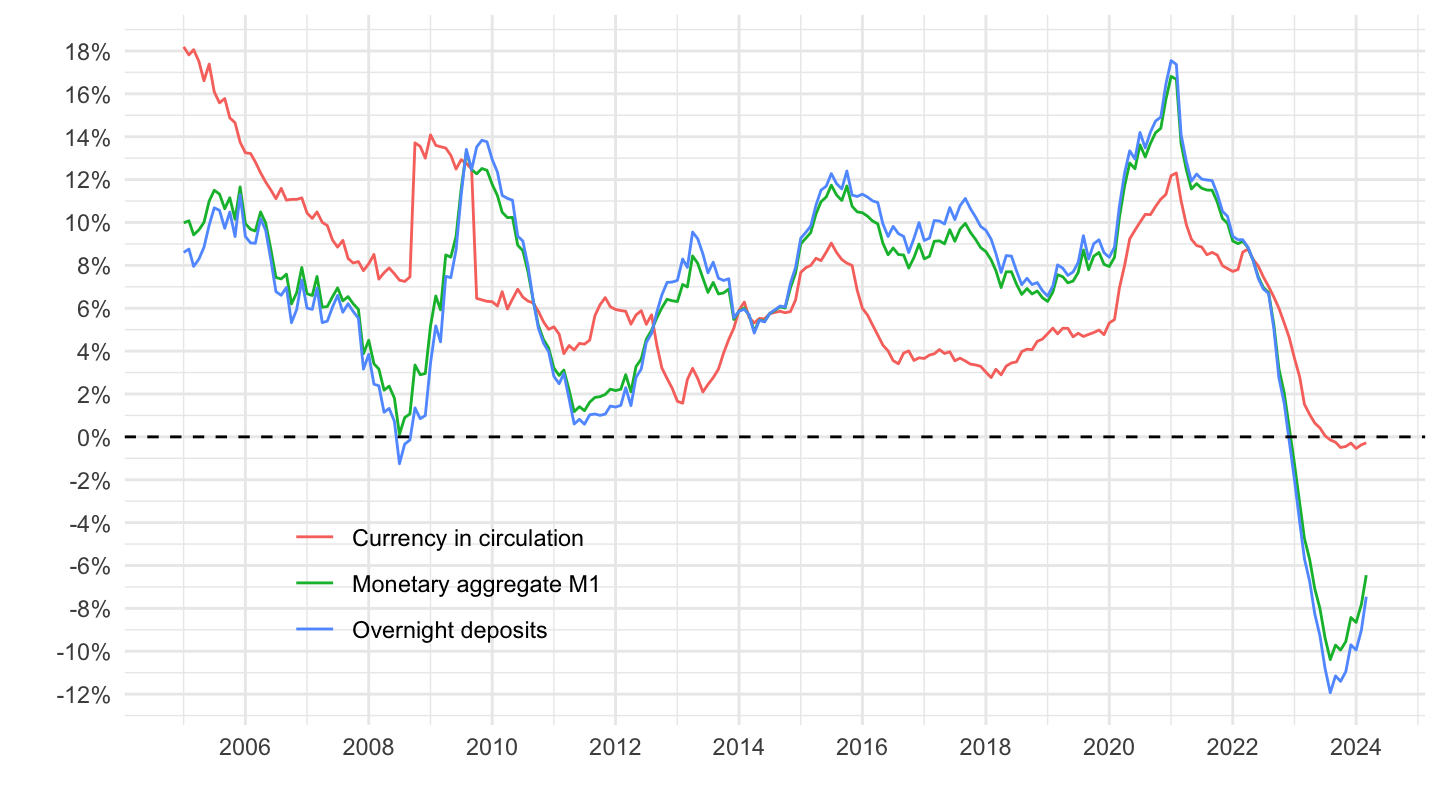
M2-M1 (other short-term deposits)
M2-M1 = deposits with an agreed maturity of up to 2 years + deposits redeemable at notice of up to 3 months
Level
Code
BSI %>%
  filter(BS_ITEM %in% c("L2A", "L22", "L23"),
         BS_COUNT_SECTOR == "2300",
         BS_SUFFIX == "E",
         FREQ == "M",
         ADJUSTMENT == "N",
         COLLECTION == "E",
         DATA_TYPE == "1",
         BS_REP_SECTOR == "V",
         REF_AREA == "U2") %>%
  left_join(BS_ITEM,  by = "BS_ITEM") %>%
  month_to_date %>%
  arrange(desc(date)) %>%
  group_by(date) %>%
  filter(n() == 3) %>%
  mutate(Bs_item = ifelse(BS_ITEM == "L2A", "Monetary aggregate M2-M1", Bs_item)) %>%
  mutate(Bs_item = factor(Bs_item, levels = c("Monetary aggregate M2-M1", "Deposits with agreed maturity", "Deposits redeemable at notice"))) %>%
  ggplot + geom_line(aes(x = date, y = OBS_VALUE/10^3, color = Bs_item)) +
  xlab("") + ylab("") + theme_minimal() +
  scale_x_date(breaks = as.Date(paste0(seq(1940, 2030, 2), "-01-01")),
               labels = date_format("%Y")) +
  theme(legend.position = c(0.2, 0.9),
        legend.title = element_blank()) +
  scale_y_continuous(breaks = 1000*seq(-100, 90, .5),
                     labels = scales::dollar_format(acc = 1, su = " Bn€", pre = ""))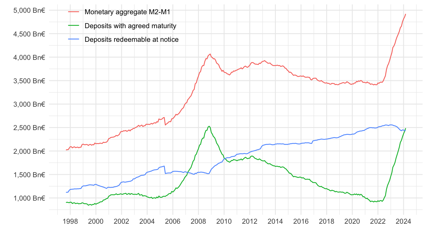
Growth
All
Code
BSI %>%
  filter(BS_ITEM %in% c("L2A", "L22", "L23"),
         BS_COUNT_SECTOR == "2300",
         BS_SUFFIX == "A",
         FREQ == "M",
         BS_REP_SECTOR == "V",
         REF_AREA == "U2",
         ADJUSTMENT == "N") %>%
  left_join(BS_ITEM,  by = "BS_ITEM") %>%
  month_to_date %>%
  arrange(desc(date)) %>%
  ggplot + geom_line(aes(x = date, y = OBS_VALUE/100, color = Bs_item)) +
  xlab("") + ylab("") + theme_minimal() +
  scale_x_date(breaks = as.Date(paste0(seq(1940, 2030, 5), "-01-01")),
               labels = date_format("%Y")) +
  theme(legend.position = c(0.25, 0.9),
        legend.title = element_blank()) +
  scale_y_continuous(breaks = 0.01*seq(-100, 90, 2),
                     labels = scales::percent_format(accuracy = 1)) +
  geom_hline(yintercept = 0, linetype = "dashed")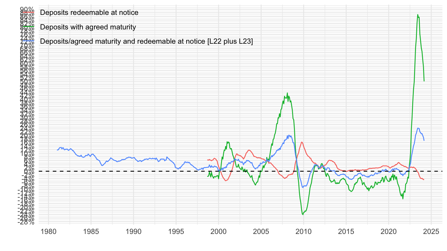
2005-
Code
BSI %>%
  filter(BS_ITEM %in% c("L2A", "L22", "L23"),
         BS_COUNT_SECTOR == "2300",
         BS_SUFFIX == "A",
         FREQ == "M",
         BS_REP_SECTOR == "V",
         REF_AREA == "U2",
         ADJUSTMENT == "N") %>%
  left_join(BS_ITEM,  by = "BS_ITEM") %>%
  month_to_date %>%
  arrange(desc(date)) %>%
  filter(date >= as.Date("2005-01-01")) %>%
  ggplot + geom_line(aes(x = date, y = OBS_VALUE/100, color = Bs_item)) +
  xlab("") + ylab("") + theme_minimal() +
  scale_x_date(breaks = as.Date(paste0(seq(1940, 2030, 2), "-01-01")),
               labels = date_format("%Y")) +
  theme(legend.position = c(0.3, 0.8),
        legend.title = element_blank()) +
  scale_y_continuous(breaks = 0.01*seq(-100, 90, 10),
                     labels = scales::percent_format(accuracy = 1)) +
  geom_hline(yintercept = 0, linetype = "dashed")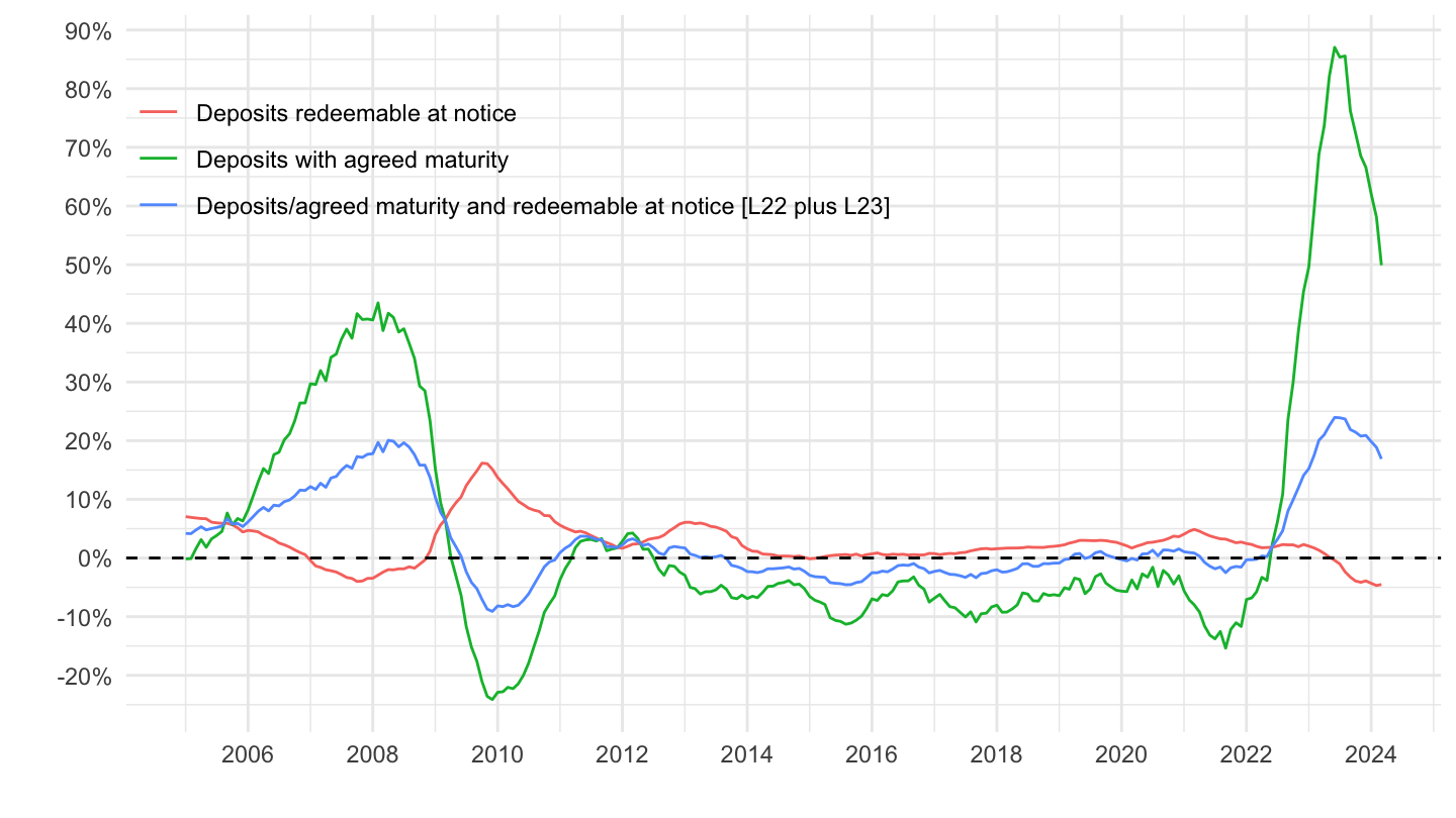
M3-M2 (marketable instruments)
M3-M2 = Repurchase agreements + money market fund shares + Debt securities with maturity of up to 2 years
Level
Code
BSI %>%
  filter(BS_ITEM %in% c("LT3", "L24A", "L40", "L30"),
         BS_COUNT_SECTOR == "2300",
         BS_SUFFIX == "E",
         FREQ == "M",
         ADJUSTMENT == "N",
         COLLECTION == "E",
         DATA_TYPE == "1",
         BS_REP_SECTOR == "V",
         REF_AREA == "U2") %>%
  left_join(BS_ITEM,  by = "BS_ITEM") %>%
  month_to_date %>%
  arrange(desc(date)) %>%
  group_by(date) %>%
  filter(n() == 4) %>%
  mutate(Bs_item = ifelse(BS_ITEM == "LT3", "Monetary aggregate M3-M2", Bs_item)) %>%
  mutate(Bs_item = factor(Bs_item, levels = c("Monetary aggregate M3-M2", "Money Market Funds shares/units", "Repurchase agreements excluding repos with central counterparties", "Debt securities issued"))) %>%
  ggplot + geom_line(aes(x = date, y = OBS_VALUE/10^3, color = Bs_item)) +
  xlab("") + ylab("") + theme_minimal() +
  scale_x_date(breaks = as.Date(paste0(seq(1940, 2030, 2), "-01-01")),
               labels = date_format("%Y")) +
  theme(legend.position = c(0.4, 0.8),
        legend.title = element_blank()) +
  scale_y_continuous(breaks = 1000*seq(-100, 90, .1),
                     labels = scales::dollar_format(acc = 1, su = " Bn€", pre = ""))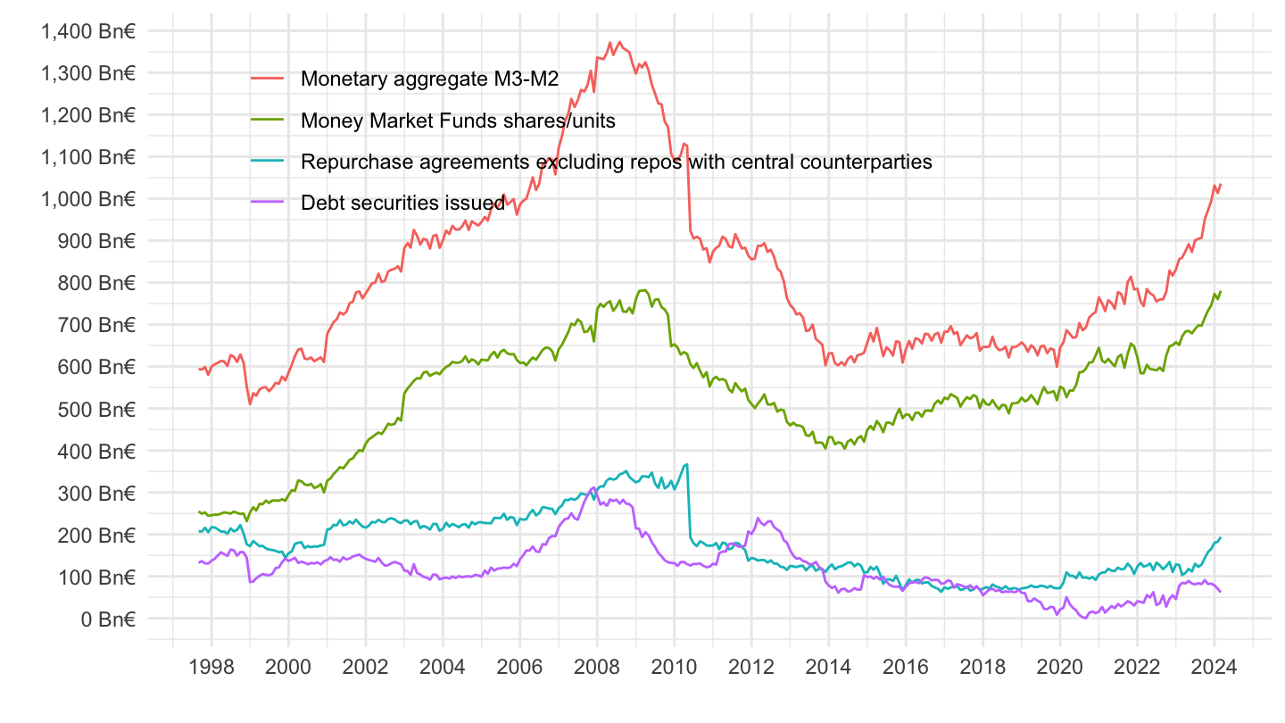
Growth
All
Code
BSI %>%
  filter(BS_ITEM %in% c("LT3", "L24A", "L40", "L30"),
         BS_COUNT_SECTOR == "2300",
         BS_SUFFIX == "A",
         FREQ == "M",
         BS_REP_SECTOR == "V",
         REF_AREA == "U2",
         ADJUSTMENT == "N") %>%
  left_join(BS_ITEM,  by = "BS_ITEM") %>%
  month_to_date %>%
  arrange(desc(date)) %>%
  ggplot + geom_line(aes(x = date, y = OBS_VALUE/100, color = Bs_item)) +
  xlab("") + ylab("") + theme_minimal() +
  scale_x_date(breaks = as.Date(paste0(seq(1940, 2030, 5), "-01-01")),
               labels = date_format("%Y")) +
  theme(legend.position = c(0.25, 0.9),
        legend.title = element_blank()) +
  scale_y_continuous(breaks = 0.01*seq(-100, 90, 2),
                     labels = scales::percent_format(accuracy = 1)) +
  geom_hline(yintercept = 0, linetype = "dashed")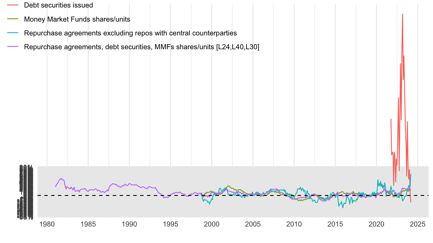
2005-
Code
BSI %>%
  filter(BS_ITEM %in% c("LT3", "L24A", "L40", "L30"),
         BS_COUNT_SECTOR == "2300",
         BS_SUFFIX == "A",
         FREQ == "M",
         BS_REP_SECTOR == "V",
         REF_AREA == "U2",
         ADJUSTMENT == "N") %>%
  left_join(BS_ITEM,  by = "BS_ITEM") %>%
  month_to_date %>%
  arrange(desc(date)) %>%
  filter(date >= as.Date("2005-01-01")) %>%
  ggplot + geom_line(aes(x = date, y = OBS_VALUE/100, color = Bs_item)) +
  xlab("") + ylab("") + theme_minimal() +
  scale_x_date(breaks = as.Date(paste0(seq(1940, 2030, 2), "-01-01")),
               labels = date_format("%Y")) +
  theme(legend.position = c(0.3, 0.8),
        legend.title = element_blank()) +
  scale_y_continuous(breaks = 0.01*seq(-100, 90, 10),
                     labels = scales::percent_format(accuracy = 1)) +
  geom_hline(yintercept = 0, linetype = "dashed")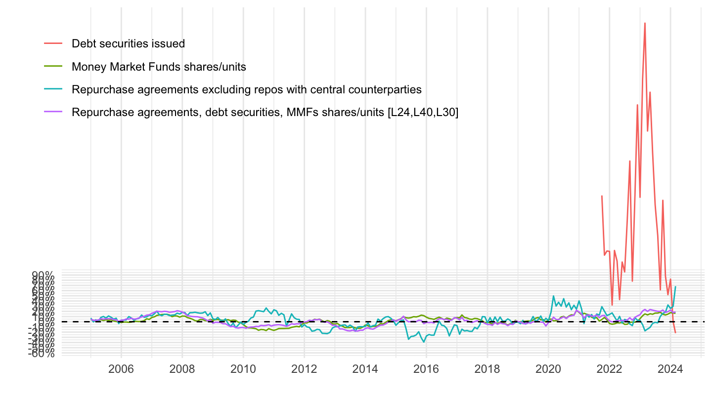
Deposits subject to reserve requirements
Total (June): 24.5 Tn€ (greater than M3)
Source: https://data.ecb.europa.eu/publications/ecbeurosystem-policy-and-exchange-rates/3030611
Liabilities to which a 1% reserve coefficient is applied
Code
BSI %>%
  filter(FREQ == "M",
         REF_AREA == "U2",
         ADJUSTMENT == "N",
         BS_REP_SECTOR == "R",
         BS_ITEM %in% c("L40", "L2B"),
         BS_SUFFIX == "E",
         BS_COUNT_SECTOR == "3000") %>%
  left_join(BS_ITEM,  by = "BS_ITEM") %>%
  month_to_date %>%
  arrange(desc(date)) %>%
  ggplot + geom_line(aes(x = date, y = OBS_VALUE/10^3, color = Bs_item)) +
  xlab("") + ylab("") + theme_minimal() +
  scale_x_date(breaks = as.Date(paste0(seq(1940, 2030, 2), "-01-01")),
               labels = date_format("%Y")) +
  theme(legend.position = c(0.4, 0.9),
        legend.title = element_blank()) +
  scale_y_continuous(breaks = 1000*seq(-100, 90, 1),
                     labels = scales::dollar_format(acc = 1, su = " Bn€", pre = ""))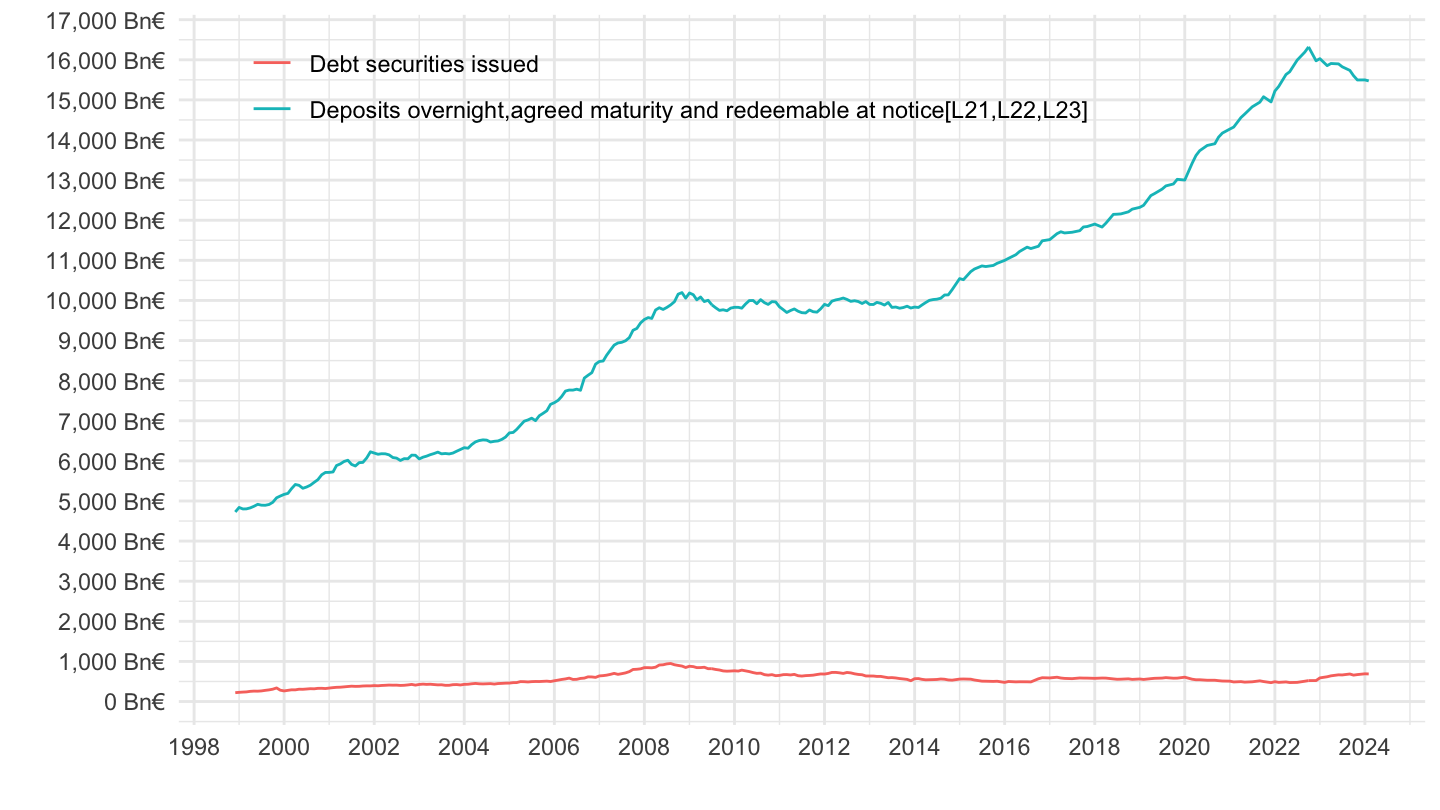
Liabilities to which a 0% reserve coefficient is applied
Code
BSI %>%
  filter(FREQ == "M",
         REF_AREA == "U2",
         ADJUSTMENT == "N",
         BS_REP_SECTOR == "R",
         BS_ITEM %in% c("L2A", "L24", "L40"),
         BS_SUFFIX == "E",
         BS_COUNT_SECTOR == "3000") %>%
  left_join(BS_ITEM,  by = "BS_ITEM") %>%
  month_to_date %>%
  arrange(desc(date)) %>%
  ggplot + geom_line(aes(x = date, y = OBS_VALUE/10^3, color = Bs_item)) +
  xlab("") + ylab("") + theme_minimal() +
  scale_x_date(breaks = as.Date(paste0(seq(1940, 2030, 2), "-01-01")),
               labels = date_format("%Y")) +
  theme(legend.position = c(0.4, 0.9),
        legend.title = element_blank()) +
  scale_y_continuous(breaks = 1000*seq(-100, 90, .2),
                     labels = scales::dollar_format(acc = 1, su = " Bn€", pre = ""))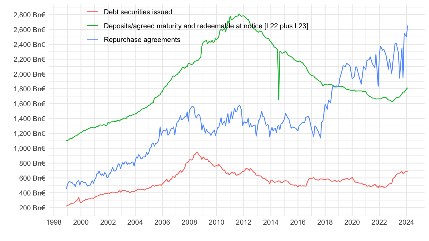
Other
Breakdown of deposits in M3: Households, NFCs, Non-MFIs (Households + NFCs)
Level
Code
BSI %>%
  filter(BS_ITEM %in% c("L2C"),
         BS_COUNT_SECTOR %in% c("2300", "2250", "2240"),
         BS_SUFFIX == "E",
         FREQ == "M",
         ADJUSTMENT == "Y",
         COLLECTION == "E",
         DATA_TYPE == "1",
         BS_REP_SECTOR == "V",
         REF_AREA == "U2") %>%
  left_join(BS_ITEM,  by = "BS_ITEM") %>%
  left_join(BS_COUNT_SECTOR,  by = "BS_COUNT_SECTOR") %>%
  month_to_date %>%
  arrange(desc(date)) %>%
  ggplot + geom_line(aes(x = date, y = OBS_VALUE/1000, color = Bs_count_sector)) +
  xlab("") + ylab("") + theme_minimal() +
  scale_x_date(breaks = as.Date(paste0(seq(1940, 2030, 2), "-01-01")),
               labels = date_format("%Y")) +
  theme(legend.position = c(0.5, 0.9),
        legend.title = element_blank()) +
  scale_y_continuous(breaks = 1000*seq(-100, 90, 1),
                     labels = scales::dollar_format(acc = 1, su = " Bn€", pre = ""))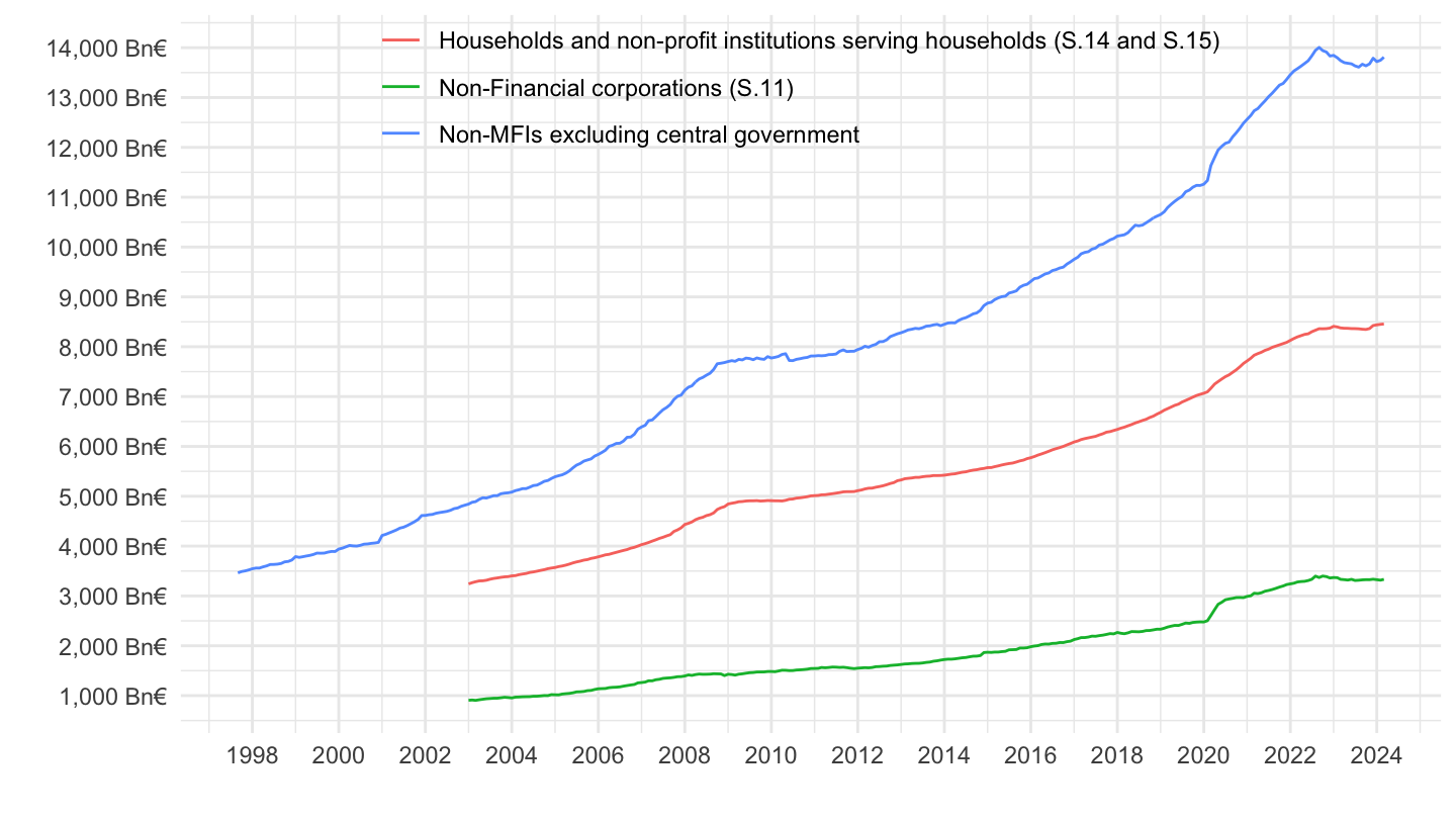
Growth
All
Code
BSI %>%
  filter(BS_ITEM %in% c("L2C"),
         BS_COUNT_SECTOR %in% c("2300", "2250", "2240"),
         BS_SUFFIX == "A",
         FREQ == "M",
         ADJUSTMENT == "Y",
         COLLECTION == "E",
         REF_AREA == "U2") %>%
  left_join(BS_ITEM,  by = "BS_ITEM") %>%
  left_join(BS_COUNT_SECTOR,  by = "BS_COUNT_SECTOR") %>%
  month_to_date %>%
  arrange(desc(date)) %>%
  ggplot + geom_line(aes(x = date, y = OBS_VALUE/100, color = Bs_count_sector)) +
  xlab("") + ylab("") + theme_minimal() +
  scale_x_date(breaks = as.Date(paste0(seq(1940, 2030, 2), "-01-01")),
               labels = date_format("%Y")) +
  theme(legend.position = c(0.4, 0.9),
        legend.title = element_blank()) +
  scale_y_continuous(breaks = 0.01*seq(-100, 90, 2),
                     labels = scales::percent_format(accuracy = 1)) +
  geom_hline(yintercept = 0, linetype = "dashed")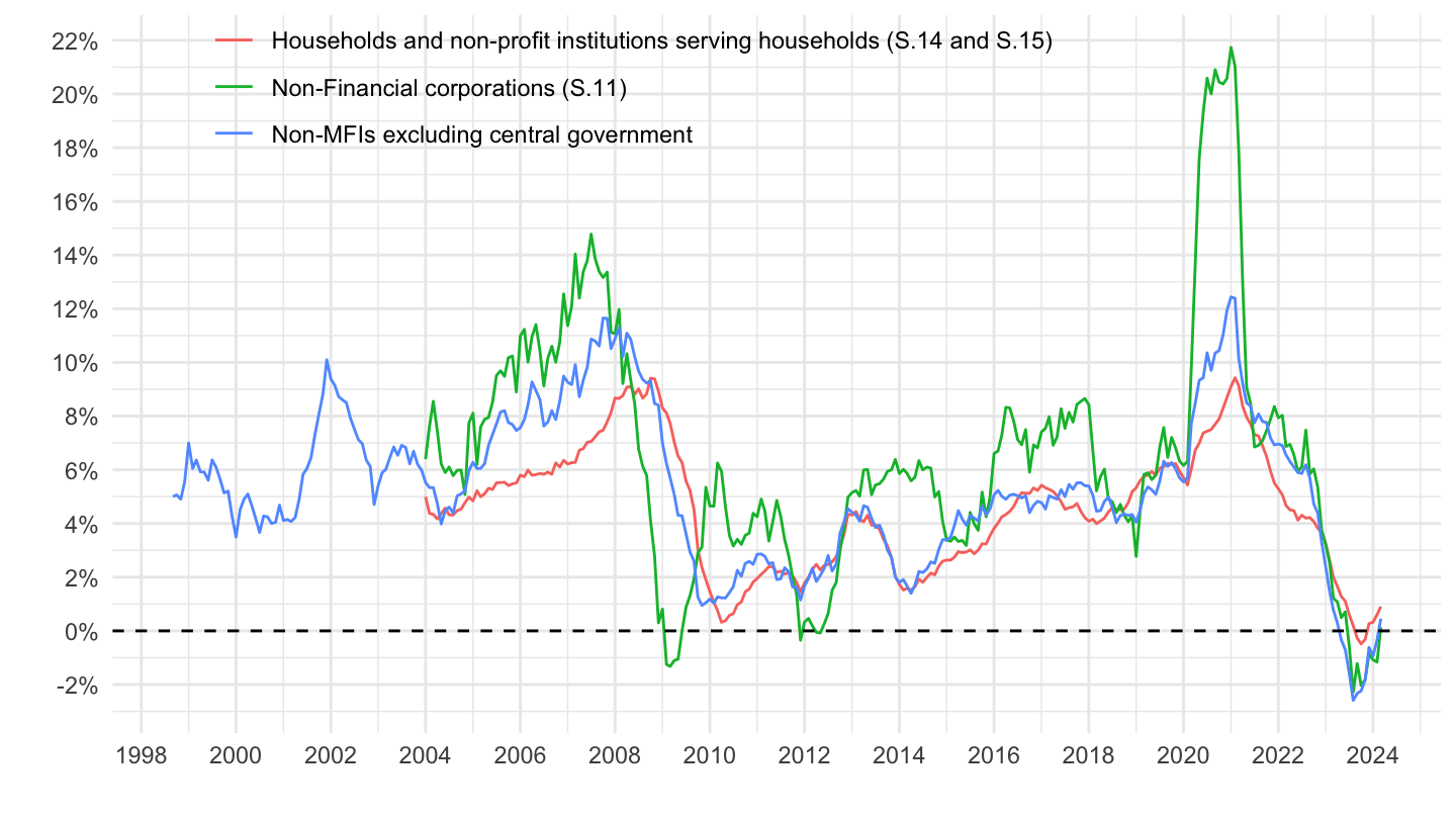
2004-
Code
BSI %>%
  filter(BS_ITEM %in% c("L2C"),
         BS_COUNT_SECTOR %in% c("2300", "2250", "2240"),
         BS_SUFFIX == "A",
         FREQ == "M",
         ADJUSTMENT == "Y",
         COLLECTION == "E",
         REF_AREA == "U2") %>%
  left_join(BS_ITEM,  by = "BS_ITEM") %>%
  left_join(BS_COUNT_SECTOR,  by = "BS_COUNT_SECTOR") %>%
  month_to_date %>%
  arrange(desc(date)) %>%
  filter(date >= as.Date("2004-01-01")) %>%
  ggplot + geom_line(aes(x = date, y = OBS_VALUE/100, color = Bs_count_sector)) +
  xlab("") + ylab("") + theme_minimal() +
  scale_x_date(breaks = as.Date(paste0(seq(1940, 2030, 2), "-01-01")),
               labels = date_format("%Y")) +
  theme(legend.position = c(0.4, 0.9),
        legend.title = element_blank()) +
  scale_y_continuous(breaks = 0.01*seq(-100, 90, 2),
                     labels = scales::percent_format(accuracy = 1)) +
  geom_hline(yintercept = 0, linetype = "dashed")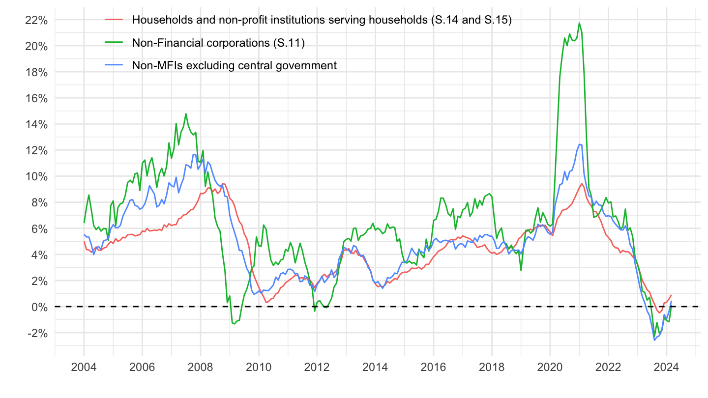
BSI.M.U2.Y.V.L2C.M.1.U2.2300.Z01.E BSI.M.U2.Y.V.L2C.M.1.U2.2250.Z01.E BSI.M.U2.Y.V.L2C.M.1.U2.2240.Z01.E
Reserves
Required reserves
Europe
Code
BSI %>%
  filter(BS_ITEM %in% c("LRE"),
         REF_AREA == "U2") %>%
  month_to_date %>%
  arrange(desc(date)) %>%
  left_join(BS_ITEM,  by = "BS_ITEM") %>%
  ggplot + geom_line(aes(x = date, y = OBS_VALUE/1000)) +
  xlab("") + ylab("Excess reserves") + theme_minimal() +
  scale_x_date(breaks = as.Date(paste0(seq(1940, 2030, 2), "-01-01")),
               labels = date_format("%Y")) +
  theme(legend.position = c(0.25, 0.9),
        legend.title = element_blank()) +
  scale_y_continuous(breaks = seq(0, 10000, 500),
                     labels = scales::dollar_format(acc = 1, su = " Bn€", pre = ""))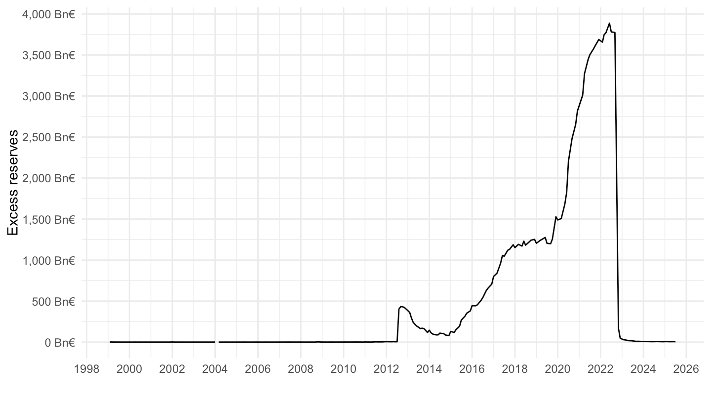
France, Germany, Italy
Code
BSI %>%
  filter(KEY %in% c("BSI.M.FR.N.R.LRE.X.1.A1.3000.Z01.E",
                    "BSI.M.DE.N.R.LRE.X.1.A1.3000.Z01.E",
                    "BSI.M.IT.N.R.LRE.X.1.A1.3000.Z01.E")) %>%
  month_to_date %>%
  left_join(REF_AREA, by = "REF_AREA") %>%
  mutate(OBS_VALUE = OBS_VALUE/100) %>%
  left_join(colors, by = c("Ref_area" = "country")) %>%
  ggplot + geom_line(aes(x = date, y = OBS_VALUE, color = color)) +
  ylab("Excess reserves in banks") + xlab("") + theme_minimal() +
  add_flags(3) + scale_color_identity() +
  theme(legend.position = c(0.45, 0.9),
        legend.title = element_blank()) +
  scale_y_continuous(breaks = seq(0, 40000, 1000),
                     labels = scales::dollar_format(acc = 1, su = " Bn€", pre = "")) +
  scale_x_date(breaks = as.Date(paste0(seq(1940, 2030, 1), "-01-01")),
               labels = date_format("%Y"))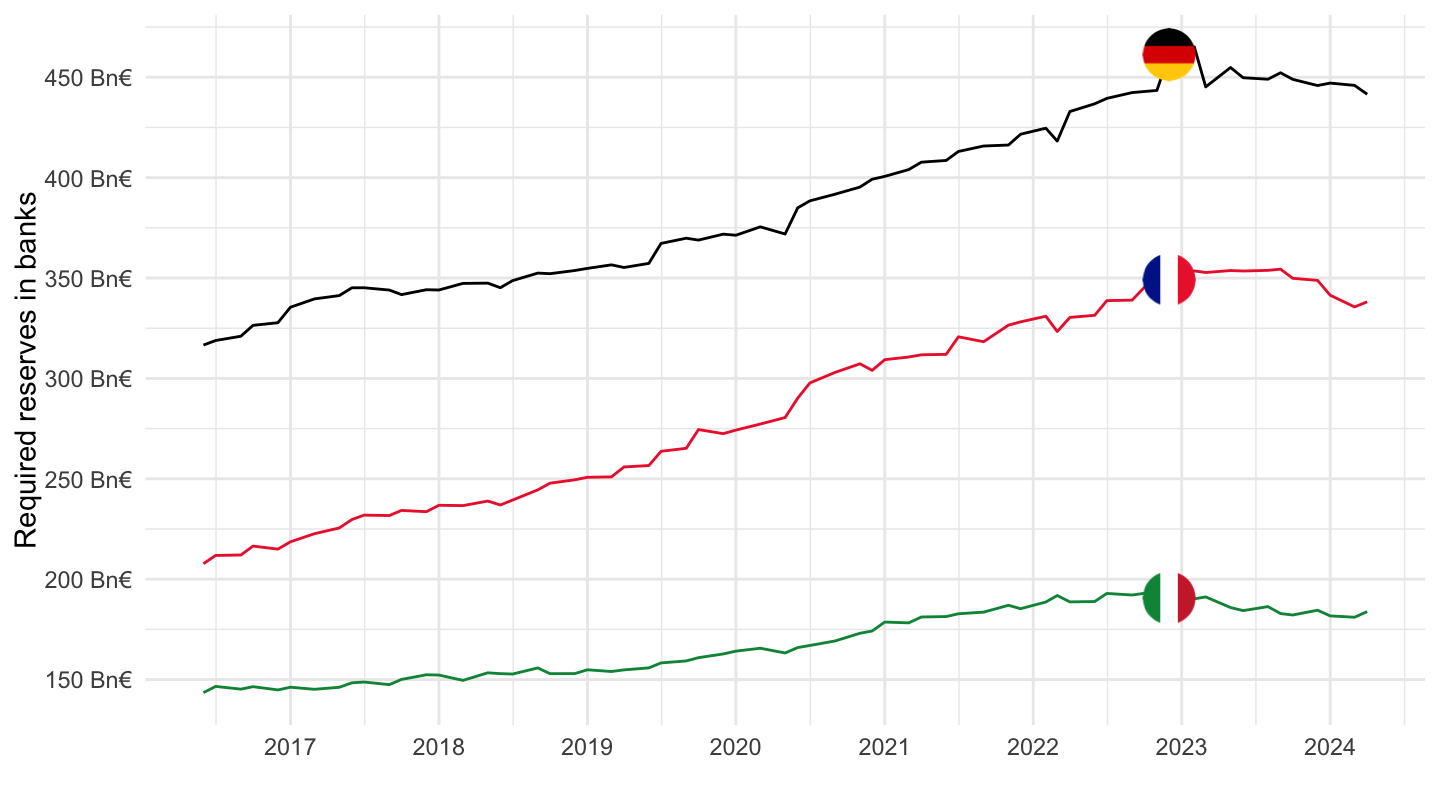
All reserves
U2 - Europe
Code
BSI %>%
  filter(BS_ITEM %in% c("LRR", "LRE"),
         REF_AREA == "U2") %>%
  month_to_date %>%
  arrange(desc(date)) %>%
  left_join(BS_ITEM,  by = "BS_ITEM") %>%
  ggplot + geom_line(aes(x = date, y = OBS_VALUE/1000, color = Bs_item)) +
  xlab("") + ylab("") + theme_minimal() +
  scale_x_date(breaks = as.Date(paste0(seq(1940, 2030, 2), "-01-01")),
               labels = date_format("%Y")) +
  theme(legend.position = c(0.25, 0.9),
        legend.title = element_blank()) +
  scale_y_continuous(breaks = seq(0, 40000, 500)) +
  geom_hline(yintercept = 0, linetype = "dashed")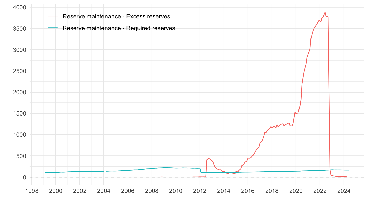
DE - Germany
Code
BSI %>%
  filter(BS_ITEM %in% c("LRR", "LRE"),
         REF_AREA == "DE") %>%
  month_to_date %>%
  arrange(desc(date)) %>%
  left_join(BS_ITEM,  by = "BS_ITEM") %>%
  ggplot + geom_line(aes(x = date, y = OBS_VALUE/1000, color = Bs_item)) +
  xlab("") + ylab("") + theme_minimal() +
  scale_x_date(breaks = as.Date(paste0(seq(1940, 2030, 2), "-01-01")),
               labels = date_format("%Y")) +
  theme(legend.position = c(0.25, 0.9),
        legend.title = element_blank()) +
  scale_y_continuous(breaks = seq(0, 40000, 100)) +
  geom_hline(yintercept = 0, linetype = "dashed")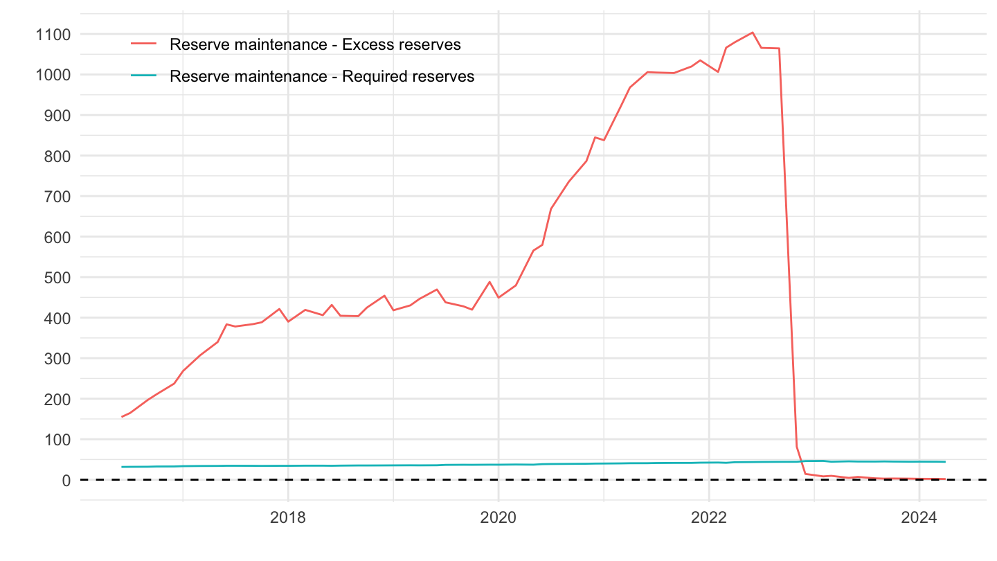
FR - Germany
Code
BSI %>%
  filter(BS_ITEM %in% c("LRR", "LRE"),
         REF_AREA == "FR") %>%
  month_to_date %>%
  arrange(desc(date)) %>%
  left_join(BS_ITEM,  by = "BS_ITEM") %>%
  ggplot + geom_line(aes(x = date, y = OBS_VALUE/1000, color = Bs_item)) +
  xlab("") + ylab("") + theme_minimal() +
  scale_x_date(breaks = as.Date(paste0(seq(1940, 2030, 2), "-01-01")),
               labels = date_format("%Y")) +
  theme(legend.position = c(0.25, 0.9),
        legend.title = element_blank()) +
  scale_y_continuous(breaks = seq(0, 40000, 100)) +
  geom_hline(yintercept = 0, linetype = "dashed")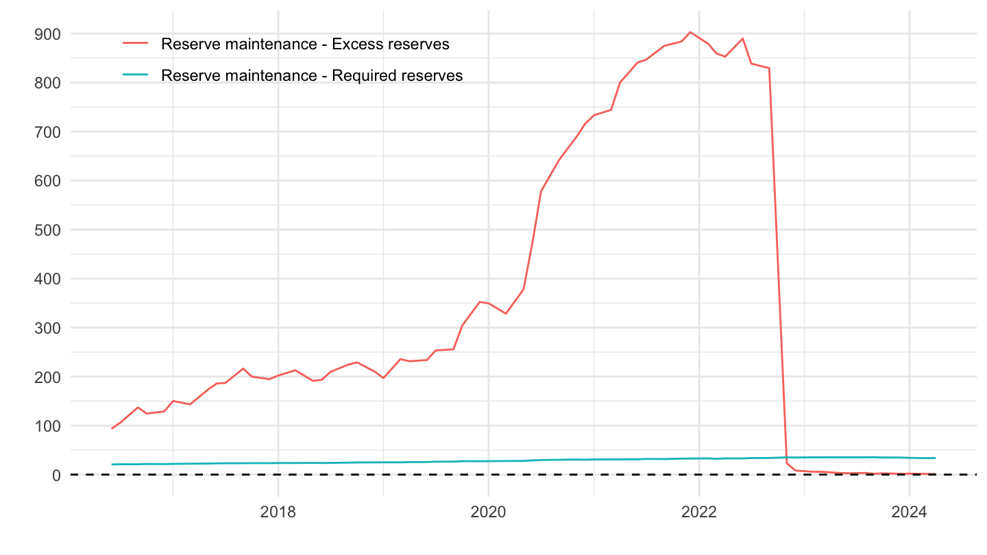
IT - Italy
Code
BSI %>%
  filter(BS_ITEM %in% c("LRR", "LRE"),
         REF_AREA == "IT") %>%
  month_to_date %>%
  arrange(desc(date)) %>%
  left_join(BS_ITEM,  by = "BS_ITEM") %>%
  ggplot + geom_line(aes(x = date, y = OBS_VALUE/1000, color = Bs_item)) +
  xlab("") + ylab("") + theme_minimal() +
  scale_x_date(breaks = as.Date(paste0(seq(1940, 2030, 2), "-01-01")),
               labels = date_format("%Y")) +
  theme(legend.position = c(0.25, 0.9),
        legend.title = element_blank()) +
  scale_y_continuous(breaks = seq(0, 40000, 100)) +
  geom_hline(yintercept = 0, linetype = "dashed")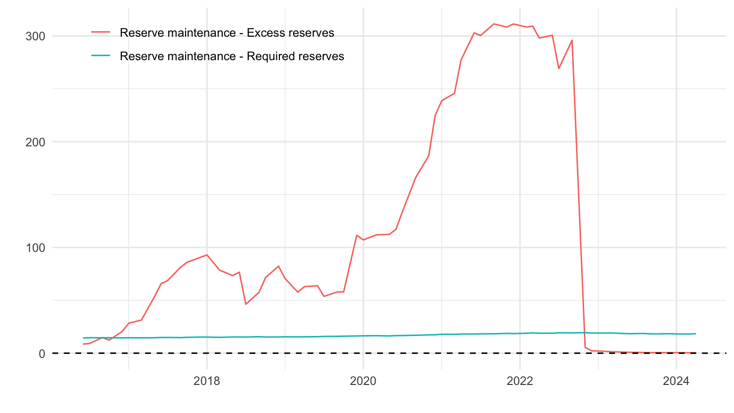
Reserve base
Code
BSI %>%
  filter(BS_ITEM %in% c("LR0")) %>%
  month_to_date %>%
  arrange(desc(date)) %>%
  left_join(BS_ITEM,  by = "BS_ITEM") %>%
  ggplot + geom_line(aes(x = date, y = OBS_VALUE/1000, color = Bs_item)) +
  xlab("") + ylab("") + theme_minimal() +
  scale_x_date(breaks = as.Date(paste0(seq(1940, 2030, 2), "-01-01")),
               labels = date_format("%Y")) +
  theme(legend.position = c(0.25, 0.9),
        legend.title = element_blank()) +
  scale_y_continuous(breaks = seq(0, 40000, 2000)) +
  geom_hline(yintercept = 0, linetype = "dashed")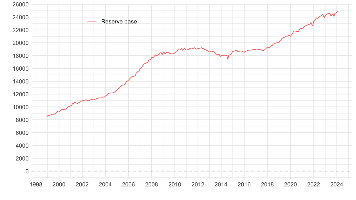
Total excess reserves of credit institutions
Excess liquidity = Excess reserves +
Europe
https://data.ecb.europa.eu/publications/money-credit-and-banking/3031796
Code
BSI %>%
  filter(KEY %in% c("BSI.M.U2.N.R.LRE.X.1.A1.3000.Z01.E")) %>%
  month_to_date %>%
  arrange(desc(date)) %>%
  left_join(BS_ITEM,  by = "BS_ITEM") %>%
  ggplot + geom_line(aes(x = date, y = OBS_VALUE/1000, color = Bs_item)) +
  xlab("") + ylab("") + theme_minimal() +
  scale_x_date(breaks = as.Date(paste0(seq(1940, 2030, 2), "-01-01")),
               labels = date_format("%Y")) +
  theme(legend.position = c(0.25, 0.9),
        legend.title = element_blank()) +
  scale_y_continuous(breaks = seq(0, 40000, 500)) +
  geom_hline(yintercept = 0, linetype = "dashed")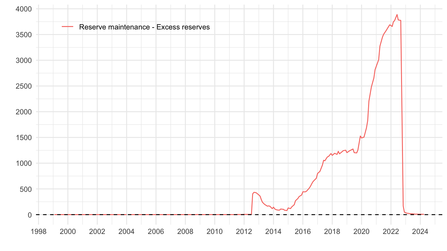
Euro area Non Financial corporations (NFCs)
France, Germany, Italy
Code
BSI %>%
  filter(KEY %in% c("BSI.M.FR.N.R.LRE.X.1.A1.3000.Z01.E",
                    "BSI.M.DE.N.R.LRE.X.1.A1.3000.Z01.E",
                    "BSI.M.IT.N.R.LRE.X.1.A1.3000.Z01.E")) %>%
  month_to_date %>%
  left_join(REF_AREA, by = "REF_AREA") %>%
  mutate(OBS_VALUE = OBS_VALUE/100) %>%
  left_join(colors, by = c("Ref_area" = "country")) %>%
  ggplot + geom_line(aes(x = date, y = OBS_VALUE, color = color)) +
  ylab("Excess reserves in banks") + xlab("") + theme_minimal() +
  add_flags(3) + scale_color_identity() +
  theme(legend.position = c(0.45, 0.9),
        legend.title = element_blank()) +
  scale_y_continuous(breaks = seq(0, 40000, 1000)) +
  scale_x_date(breaks = as.Date(paste0(seq(1940, 2030, 1), "-01-01")),
               labels = date_format("%Y"))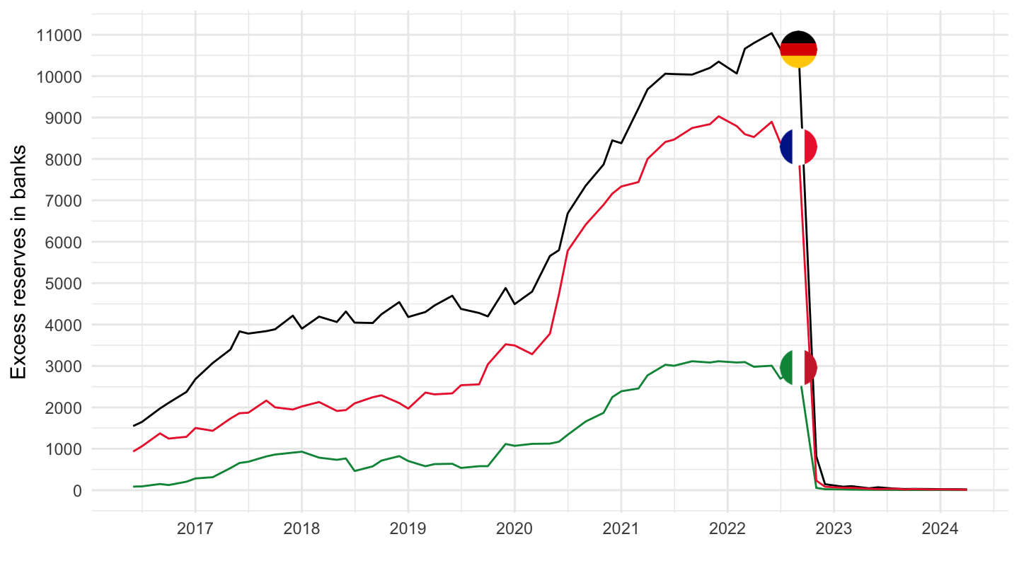
Spain, Netherlands, Portugal
Code
BSI %>%
  filter(KEY %in% c("BSI.M.ES.N.R.LRE.X.1.A1.3000.Z01.E",
                    "BSI.M.NL.N.R.LRE.X.1.A1.3000.Z01.E",
                    "BSI.M.PT.N.R.LRE.X.1.A1.3000.Z01.E")) %>%
  month_to_date %>%
  left_join(REF_AREA, by = "REF_AREA") %>%
  mutate(OBS_VALUE = OBS_VALUE/100) %>%
  left_join(colors, by = c("Ref_area" = "country")) %>%
  ggplot + geom_line(aes(x = date, y = OBS_VALUE, color = color)) +
  ylab("Excess reserves in banks") + xlab("") + theme_minimal() +
  add_flags(3) + scale_color_identity() +
  theme(legend.position = c(0.45, 0.9),
        legend.title = element_blank()) +
  scale_y_continuous(breaks = seq(0, 40000, 500)) +
  scale_x_date(breaks = as.Date(paste0(seq(1940, 2030, 1), "-01-01")),
               labels = date_format("%Y"))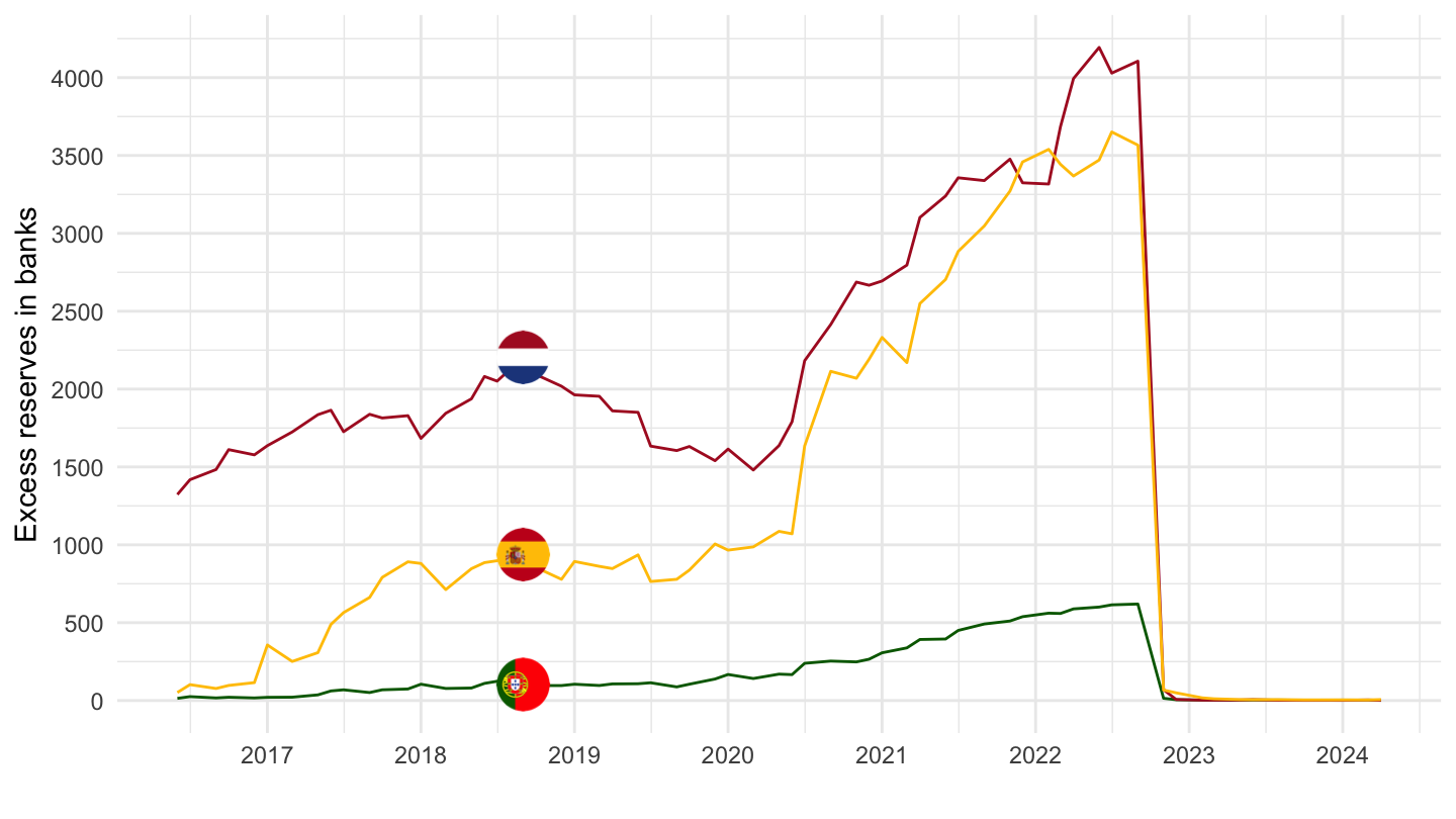
Excess reserves
Code
BSI %>%
  filter(KEY %in% c("BSI.M.FR.N.A.A20T.A.I.U2.2240.Z01.A",
                    "BSI.M.IT.N.A.A20T.A.I.U2.2240.Z01.A",
                    "BSI.M.DE.N.A.A20T.A.I.U2.2240.Z01.A")) %>%
  month_to_date %>%
  left_join(REF_AREA, by = "REF_AREA") %>%
  mutate(OBS_VALUE = OBS_VALUE/100) %>%
  left_join(colors, by = c("Ref_area" = "country")) %>%
  ggplot + geom_line(aes(x = date, y = OBS_VALUE, color = color)) +
  ylab("Adjusted loans vs. € area NFCs, annual growth") + xlab("") + theme_minimal() +
  add_flags(3) + scale_color_identity() +
  theme(legend.position = c(0.45, 0.9),
        legend.title = element_blank()) +
  scale_y_continuous(breaks = 0.01*seq(-100, 90, 2),
                     labels = scales::percent_format(accuracy = 1)) +
  scale_x_date(breaks = as.Date(paste0(seq(1940, 2030, 2), "-01-01")),
               labels = date_format("%Y"))