Supervisory Banking Statistics

Data - ECB

Author

Error in readChar(con, 5L, useBytes = TRUE) : 
  impossible d'ouvrir la connexion

Info

source	dataset	Title	.html	.rData
ecb	SUP	Supervisory Banking Statistics	2026-07-23	2026-07-23

Data on monetary policy

source	dataset	Title	Download	Compile
ecb	SUP	Supervisory Banking Statistics	2025-08-28	[2026-07-23]
bdf	FM	Marché financier, taux	2026-07-22	[2026-07-23]
bdf	MIR	Taux d'intérêt - Zone euro	2026-07-22	[2026-07-23]
bdf	MIR1	Taux d'intérêt - France	2026-07-23	[2026-07-23]
bis	CBPOL	Policy Rates, Daily	2026-07-23	[2026-07-18]
ecb	BSI	Balance Sheet Items	NA	[2026-07-24]
ecb	BSI_PUB	Balance Sheet Items - Published series	NA	[2026-07-24]
ecb	FM	Financial market data	NA	[2026-07-24]
ecb	ILM	Internal Liquidity Management	NA	[2026-07-24]
ecb	ILM_PUB	Internal Liquidity Management - Published series	2024-09-10	[2026-07-24]
ecb	MIR	MFI Interest Rate Statistics	2025-08-28	[2026-07-24]
ecb	RAI	Risk Assessment Indicators	2025-08-28	[2026-07-24]
ecb	YC	Financial market data - yield curve	NA	[2026-07-23]
ecb	YC_PUB	Financial market data - yield curve - Published series	NA	[2026-07-23]
ecb	liq_daily	Daily Liquidity	2026-07-24	[2026-07-24]
eurostat	ei_mfir_m	Interest rates - monthly data	NA	[2026-07-23]
eurostat	irt_st_m	Money market interest rates - monthly data	NA	[2026-07-24]
fred	r	Interest Rates	2026-07-23	[2026-07-23]
oecd	MEI	Main Economic Indicators	2025-07-24	[2024-04-16]
oecd	MEI_FIN	Monthly Monetary and Financial Statistics (MEI)	2025-07-24	[2024-09-15]

LAST_COMPILE

LAST_COMPILE
2026-07-24

Last

Code

SUP %>%
  group_by(TIME_PERIOD, FREQ) %>%
  summarise(Nobs = n()) %>%
  ungroup %>%
  group_by(FREQ) %>%
  arrange(desc(TIME_PERIOD)) %>%
  filter(row_number() == 1) %>%
  print_table_conditional()

TIME_PERIOD	FREQ	Nobs
2026-Q1	Q	21498
2025-S2	H	2626

Info

Data Structure Definition (DSD). html

TITLE

Code

SUP %>%
  group_by(TITLE) %>%
  summarise(Nobs = n()) %>%
  arrange(-Nobs) %>%
  {if (is_html_output()) datatable(., filter = 'top', rownames = F) else .}

BS_SUFFIX

Code

SUP %>%
  left_join(BS_SUFFIX,  by = "BS_SUFFIX") %>%
  group_by(BS_SUFFIX, Bs_suffix) %>%
  summarise(Nobs = n()) %>%
  arrange(-Nobs) %>%
  print_table_conditional()

BS_SUFFIX	Bs_suffix	Nobs
E	Euro	414906
PCT	Percentage	133784
LAF	NA	36849
Z	Not applicable	17856

CB_EXP_TYPE

Code

SUP %>%
  left_join(CB_EXP_TYPE,  by = "CB_EXP_TYPE") %>%
  group_by(CB_EXP_TYPE, Cb_exp_type) %>%
  summarise(Nobs = n()) %>%
  arrange(-Nobs) %>%
  print_table_conditional()

CB_EXP_TYPE	Cb_exp_type	Nobs
ALL	All exposures	411191
_Z	Not applicable	138271
N_	Non-performing exposures	22768
ST2	Assets with significant increase in credit risk since initial recognition but not credit-impaired (Stage 2)	11516
P_	Performing exposures	5114
NFM	Non-performing exposures with forbearance measures	4456
PFM	Performing exposures with forbearance measures	4449
ST1	Assets without significant increase in credit risk since initial recognition (Stage 1)	1986
ST3	Credit-impaired assets (Stage 3)	1986
PCI	Purchased or originated credit-impaired financial assets	1658

CB_ITEM

Code

SUP %>%
  left_join(CB_ITEM,  by = "CB_ITEM") %>%
  group_by(CB_ITEM, Cb_item) %>%
  summarise(Nobs = n()) %>%
  arrange(-Nobs) %>%
  print_table_conditional()

SBS_DI_1

Code

SUP %>%
  left_join(SBS_DI_1,  by = "SBS_DI_1") %>%
  group_by(SBS_DI_1, Sbs_di_1) %>%
  summarise(Nobs = n()) %>%
  arrange(-Nobs) %>%
  print_table_conditional()

SBS_DI_1	Sbs_di_1	Nobs
SII	Significant institutions	419152
LSI	Less significant institutions	150147
ALL	NA	34096

SBS_BREAKDOWN

Code

SUP %>%
  left_join(SBS_BREAKDOWN,  by = "SBS_BREAKDOWN") %>%
  group_by(SBS_BREAKDOWN, Sbs_breakdown) %>%
  summarise(Nobs = n()) %>%
  arrange(-Nobs) %>%
  print_table_conditional()

SBS_BREAKDOWN	Sbs_breakdown	Nobs
_T	Total	358994
AMC	Classification by business model - asset manager & custodian	15344
CWH	Classification by business model - corporate/wholesale lenders	15344
DEV	Classification by business model - development/promotional lenders	15344
DIV	Classification by business model - diversified lenders	15344
NC	Classification by business model - others/ not classified	15344
RCCL	Classification by business model - retail lenders and consumer credit lenders	15344
UNI	Classification by business model - universal and investment banks	15344
GSIB	Classification by size/business model - G-SIBs	10968
SML	Classification by business model - small market lenders	10611
SL30	Classification by size - banks with total assets less than 30 billion of EUR	9698
SM20	Classification by size - banks with total assets more than 200 billion of EUR	9698
ST10	Classification by size - banks with total assets between 30 billion and 100 billion of EUR	9698
ST20	Classification by size - banks with total assets between 100 billion and 200 billion of EUR	9698
LORI	Classification by risk - banks with low risk	9341
MHRI	Classification by risk - banks with medium, high risk and non-rated	9341
DOM	Classification by geographical diversification - banks with significant domestic exposures	9292
EEA	Classification by geographical diversification - banks with largest non-domestic exposures in non-SSM EEA	9292
NEEA	Classification by geographical diversification - banks with largest non-domestic exposures in non-EEA Europe	9292
ROW	Classification by geographical diversification - banks with largest non-domestic exposures in RoW	9292
SSM	Classification by geographical diversification - banks with largest non-domestic exposures in the SSM	9292
CSCB	Classification by business model-central savings and cooperative banks	5740
EML	Classification by business model-emerging markets lenders	5740

COUNT_AREA

Code

SUP %>%
  left_join(COUNT_AREA,  by = "COUNT_AREA") %>%
  group_by(COUNT_AREA, Count_area) %>%
  summarise(Nobs = n()) %>%
  arrange(-Nobs) %>%
  print_table_conditional()

FREQ

Code

SUP %>%
  left_join(FREQ,  by = "FREQ") %>%
  group_by(FREQ, Freq) %>%
  summarise(Nobs = n()) %>%
  arrange(-Nobs) %>%
  print_table_conditional()

FREQ	Freq	Nobs
Q	Quarterly	577335
H	Half-yearly	26060

REF_AREA

Code

SUP %>%
  left_join(REF_AREA,  by = "REF_AREA") %>%
  group_by(REF_AREA, Ref_area) %>%
  summarise(Nobs = n()) %>%
  arrange(-Nobs) %>%
  print_table_conditional()

REF_AREA	Ref_area	Nobs
B01	EU countries participating in the Single Supervisory Mechanism (SSM) (changing composition)	277939
AT	Austria	15884
BE	Belgium	15884
CY	Cyprus	15884
DE	Germany	15884
EE	Estonia	15884
ES	Spain	15884
FI	Finland	15884
FR	France	15884
GR	Greece	15884
IE	Ireland	15884
IT	Italy	15884
LT	Lithuania	15884
LU	Luxembourg	15884
LV	Latvia	15884
MT	Malta	15884
NL	Netherlands	15884
PT	Portugal	15884
SI	Slovenia	15884
SK	Slovakia	15884
BG	Bulgaria	11830
HR	Croatia	11830

COUNTERPART_SECTOR

Code

SUP %>%
  left_join(COUNTERPART_SECTOR,  by = "COUNTERPART_SECTOR") %>%
  group_by(COUNTERPART_SECTOR, Counterpart_sector) %>%
  summarise(Nobs = n()) %>%
  arrange(-Nobs) %>%
  print_table_conditional()

COUNTERPART_SECTOR	Counterpart_sector	Nobs
_Z	Not applicable	471243
S13	General government	34831
S11	Non financial corporations	29612
S14	Households	27706
S12R	Other financial corporations	14412
S122Z	Deposit-taking corporations except the central bank and excluding electronic money institutions principally engaged in financial intermediation	8764
S121	Central bank	8733
S1V	Non-financial corporations, households and NPISH	8094

TIME_FORMAT

Code

SUP %>%
  group_by(TIME_FORMAT) %>%
  summarise(Nobs = n()) %>%
  arrange(-Nobs) %>%
  print_table_conditional()

TIME_FORMAT	Nobs
P3M	577335
P6M	26060

Performance Indicators

https://www.bankingsupervision.europa.eu/banking/statistics/html/index.en.html

Return on equity

Graph

significant institutions (SIs) and less significant institutions (LSIs):

Code

SUP %>%
  filter(grepl("Return on equity", TITLE),
         REF_AREA %in% c("U2", "FR", "IT", "DE"),
         BS_SUFFIX == "PCT") %>%
  left_join(REF_AREA, by = "REF_AREA") %>%
  left_join(SBS_DI_1,  by = "SBS_DI_1") %>%
  quarter_to_date %>%
  select_if(~ n_distinct(.) > 1) %>%
  left_join(colors, by = c("Ref_area" = "country")) %>%
  mutate(OBS_VALUE = OBS_VALUE/100) %>%
  ggplot(.) + theme_minimal() + xlab("") + ylab("Return on equity") +
  geom_line(aes(x = date, y = OBS_VALUE, color = color, linetype = Sbs_di_1)) + 
  add_flags(7) + scale_color_identity() +
  scale_x_date(breaks = seq(1960, 2100, 1) %>% paste0("-01-01") %>% as.Date,
               labels = date_format("%Y")) +
  scale_y_continuous(breaks = 0.01*seq(-100, 100, 2),
                     labels = percent_format(accuracy = 1)) +
  theme(legend.position = c(0.25, 0.90),
        legend.title = element_blank())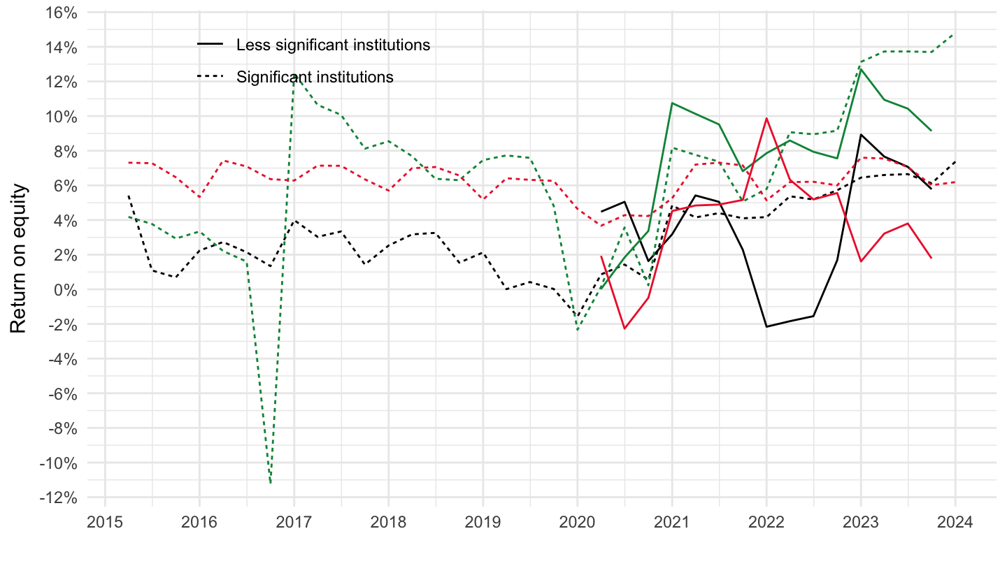

Cost-to-income ratio

Code

SUP %>%
  filter(grepl("Cost-to-income ratio", TITLE),
         REF_AREA %in% c("U2", "FR", "IT", "DE"),
         BS_SUFFIX == "PCT") %>%
  left_join(REF_AREA, by = "REF_AREA") %>%
  left_join(SBS_DI_1,  by = "SBS_DI_1") %>%
  quarter_to_date %>%
  select_if(~ n_distinct(.) > 1) %>%
  left_join(colors, by = c("Ref_area" = "country")) %>%
  mutate(OBS_VALUE = OBS_VALUE/100) %>%
  ggplot(.) + theme_minimal() + xlab("") + ylab("Cost-to-income Ratio") +
  geom_line(aes(x = date, y = OBS_VALUE, color = color, linetype = Sbs_di_1)) + 
  add_flags(7) + scale_color_identity() +
  scale_x_date(breaks = seq(1960, 2100, 1) %>% paste0("-01-01") %>% as.Date,
               labels = date_format("%Y")) +
  scale_y_continuous(breaks = 0.01*seq(-10, 100, 10),
                     labels = percent_format(accuracy = .1)) +
  theme(legend.position = c(0.25, 0.90),
        legend.title = element_blank())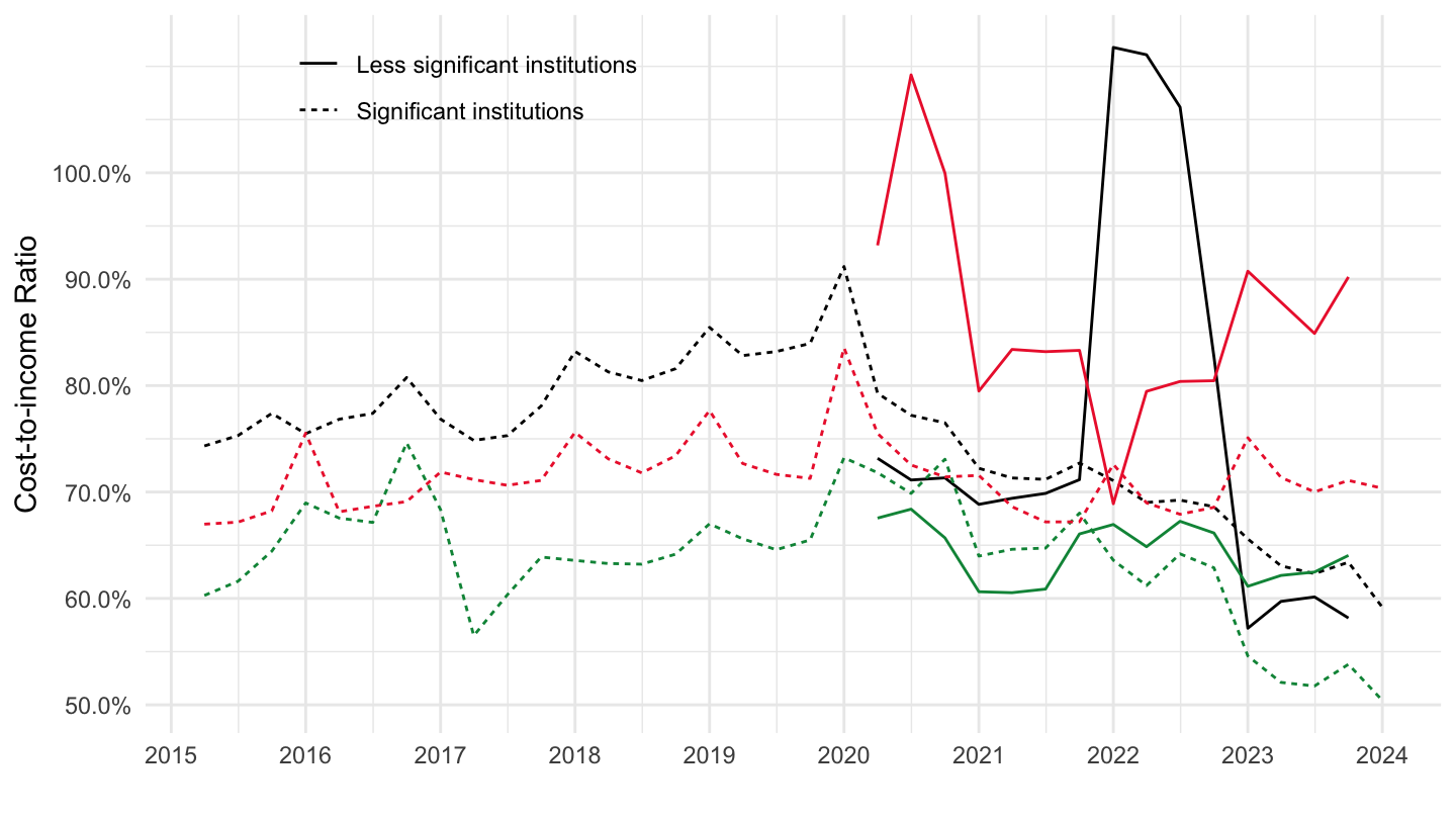

Net interest income

FR, IT, DE

Code

SUP %>%
  filter(grepl("Net interest income", TITLE),
         REF_AREA %in% c("U2", "FR", "IT", "DE"),
         BS_SUFFIX == "PCT") %>%
  left_join(REF_AREA, by = "REF_AREA") %>%
  left_join(SBS_DI_1,  by = "SBS_DI_1") %>%
  quarter_to_date %>%
  select_if(~ n_distinct(.) > 1) %>%
  left_join(colors, by = c("Ref_area" = "country")) %>%
  mutate(OBS_VALUE = OBS_VALUE/100) %>%
  ggplot(.) + theme_minimal() + xlab("") + ylab("Net Interest Income/Total operating income") +
  geom_line(aes(x = date, y = OBS_VALUE, color = color, linetype = Sbs_di_1)) + 
  add_flags(7) + scale_color_identity() +
  scale_x_date(breaks = seq(1960, 2100, 1) %>% paste0("-01-01") %>% as.Date,
               labels = date_format("%Y")) +
  scale_y_continuous(breaks = 0.01*seq(-10, 100, 10),
                     labels = percent_format(accuracy = .1)) +
  theme(legend.position = c(0.25, 0.90),
        legend.title = element_blank())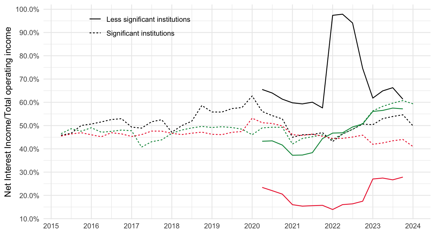

FR, IT, DE, ES, NL, SI

Net interest margin

FR, IT, DE

Code

SUP %>%
  filter(grepl("Net interest margin", TITLE),
         REF_AREA %in% c("U2", "FR", "IT", "DE")) %>%
  left_join(REF_AREA, by = "REF_AREA") %>%
  left_join(SBS_DI_1,  by = "SBS_DI_1") %>%
  quarter_to_date %>%
  select_if(~ n_distinct(.) > 1) %>%
  left_join(colors, by = c("Ref_area" = "country")) %>%
  mutate(OBS_VALUE = OBS_VALUE/100) %>%
  ggplot(.) + theme_minimal() + xlab("") + ylab("Net Interest Margin") +
  geom_line(aes(x = date, y = OBS_VALUE, color = color, linetype = Sbs_di_1)) + 
  add_flags(6) + scale_color_identity() +
  scale_x_date(breaks = seq(1960, 2100, 1) %>% paste0("-01-01") %>% as.Date,
               labels = date_format("%Y")) +
  scale_y_continuous(breaks = 0.01*seq(-10, 50, 0.1),
                     labels = percent_format(accuracy = .1)) +
  theme(legend.position = c(0.25, 0.90),
        legend.title = element_blank())

FR, IT, DE, ES, NL, SI

Code

SUP %>%
  filter(grepl("Net interest margin", TITLE),
         REF_AREA %in% c("U2", "FR", "IT", "DE", "ES", "NL", "SI"),
         SBS_DI_1 == "SII") %>%
  left_join(REF_AREA, by = "REF_AREA") %>%
  quarter_to_date %>%
  arrange(desc(date)) %>%
  left_join(SBS_DI_1,  by = "SBS_DI_1") %>%
  select_if(~ n_distinct(.) > 1) %>%
  left_join(colors, by = c("Ref_area" = "country")) %>%
  mutate(OBS_VALUE = OBS_VALUE/100) %>%
  ggplot(.) + theme_minimal() + xlab("") + ylab("Net Interest Margin") +
  geom_line(aes(x = date, y = OBS_VALUE, color = color)) + 
  add_flags(6) + scale_color_identity() +
  scale_x_date(breaks = seq(1960, 2100, 1) %>% paste0("-01-01") %>% as.Date,
               labels = date_format("%Y")) +
  scale_y_continuous(breaks = 0.01*seq(-10, 50, 0.1),
                     labels = percent_format(accuracy = .1)) +
  theme(legend.position = c(0.25, 0.90),
        legend.title = element_blank())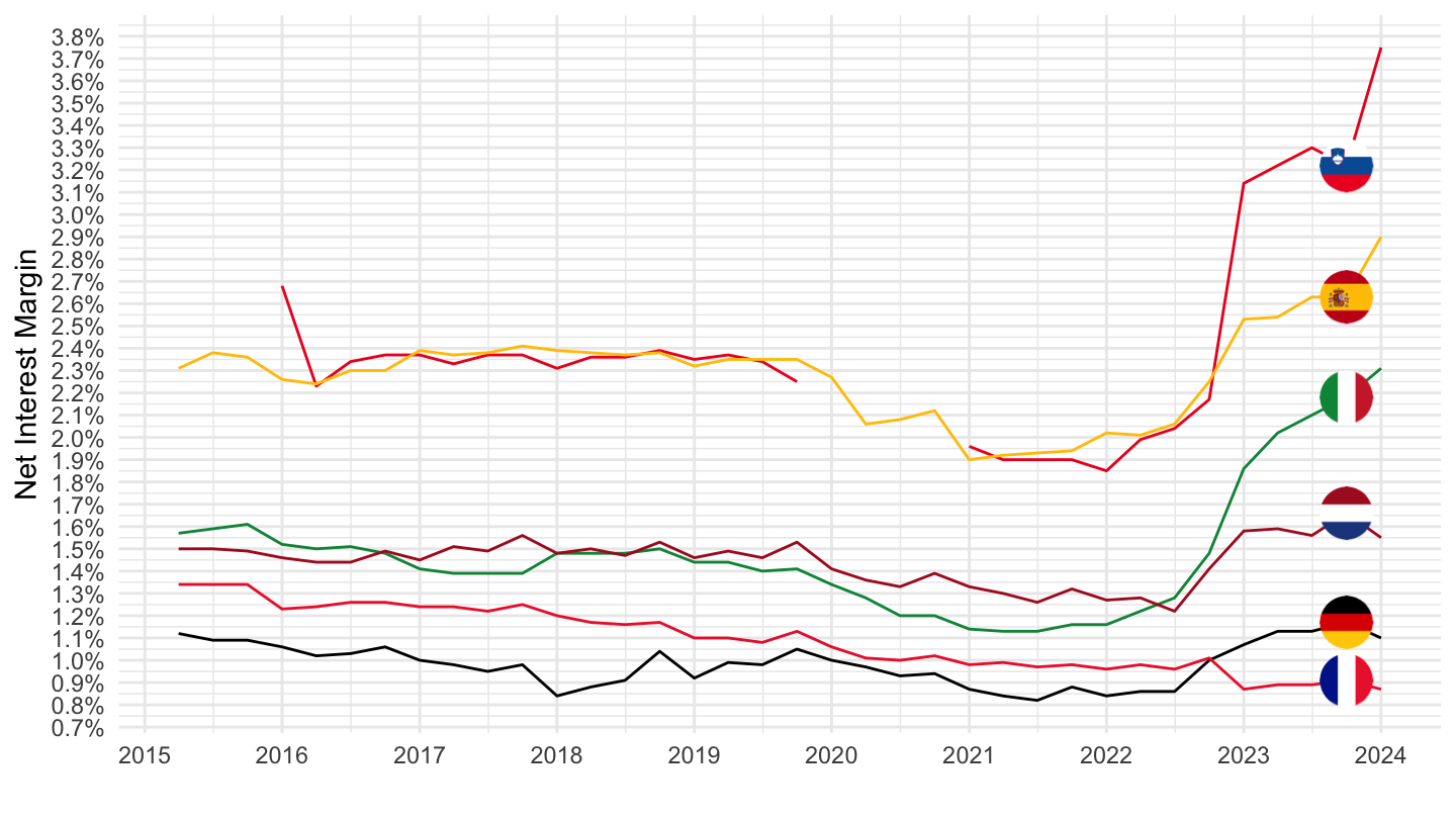

FR, IT, DE, ES, NL, BE, AT, PT

2015-

Code

SUP %>%
  filter(grepl("Net interest margin", TITLE),
         REF_AREA %in% c("U2", "FR", "IT", "DE", "ES", "NL", "BE", "AT", "PT"),
         SBS_DI_1 == "SII") %>%
  left_join(REF_AREA, by = "REF_AREA") %>%
  quarter_to_date %>%
  arrange(desc(date)) %>%
  left_join(SBS_DI_1,  by = "SBS_DI_1") %>%
  select_if(~ n_distinct(.) > 1) %>%
  left_join(colors, by = c("Ref_area" = "country")) %>%
  mutate(OBS_VALUE = OBS_VALUE/100) %>%
  mutate(color = ifelse(REF_AREA == "FR", color2, color)) %>%
  ggplot(.) + theme_minimal() + xlab("") + ylab("Net Interest Margin") +
  geom_line(aes(x = date, y = OBS_VALUE, color = color)) + 
  add_flags(8) + scale_color_identity() +
  scale_x_date(breaks = seq(1960, 2100, 1) %>% paste0("-01-01") %>% as.Date,
               labels = date_format("%Y")) +
  scale_y_continuous(breaks = 0.01*seq(-10, 50, 0.1),
                     labels = percent_format(accuracy = .1)) +
  theme(legend.position = c(0.25, 0.90),
        legend.title = element_blank())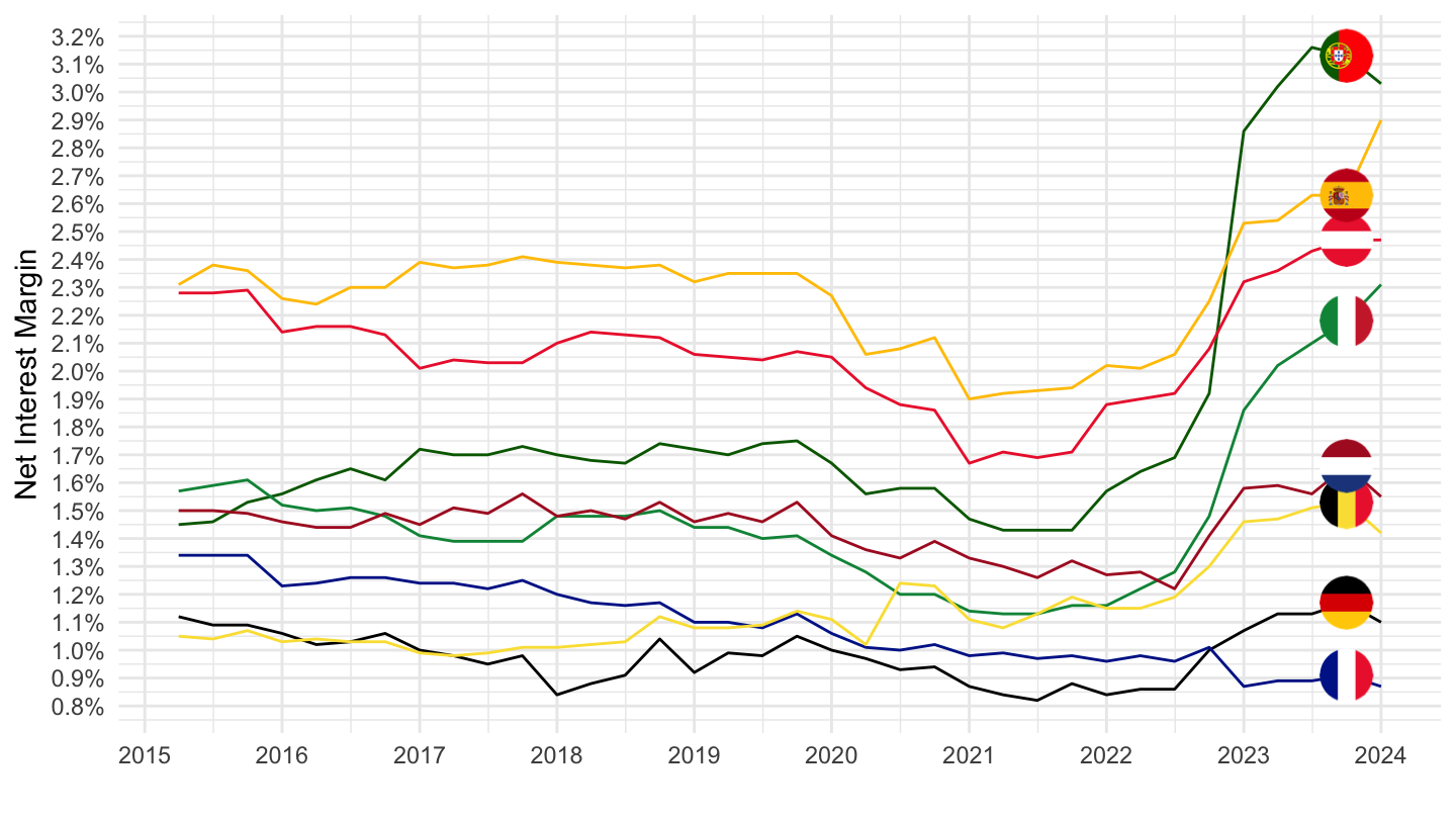

2018-

Code

SUP %>%
  filter(grepl("Net interest margin", TITLE),
         REF_AREA %in% c("U2", "FR", "IT", "DE", "ES", "NL", "BE", "AT", "PT"),
         SBS_DI_1 == "SII") %>%
  left_join(REF_AREA, by = "REF_AREA") %>%
  quarter_to_date %>%
  filter(date >= as.Date("2018-01-01")) %>%
  arrange(desc(date)) %>%
  left_join(SBS_DI_1,  by = "SBS_DI_1") %>%
  select_if(~ n_distinct(.) > 1) %>%
  left_join(colors, by = c("Ref_area" = "country")) %>%
  mutate(OBS_VALUE = OBS_VALUE/100) %>%
  mutate(color = ifelse(REF_AREA == "FR", color2, color)) %>%
  ggplot(.) + theme_minimal() + xlab("") + ylab("Net Interest Margin") +
  geom_line(aes(x = date, y = OBS_VALUE, color = color)) + 
  add_flags(8) + scale_color_identity() +
  scale_x_date(breaks = seq(1960, 2100, 1) %>% paste0("-01-01") %>% as.Date,
               labels = date_format("%Y")) +
  scale_y_continuous(breaks = 0.01*seq(-10, 50, 0.1),
                     labels = percent_format(accuracy = .1)) +
  theme(legend.position = c(0.25, 0.90),
        legend.title = element_blank())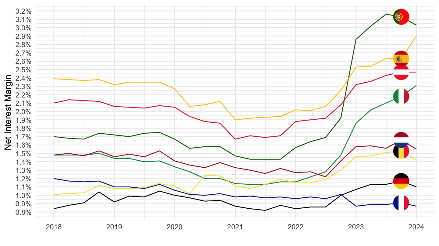

Liquidity

Liquidity coverage ratios (LCR)

The LCR is the percentage resulting from dividing the bank’s stock of high-quality assets by the estimated total net cash outflows over a 30 calendar day stress scenario.

Code

SUP %>%
  filter(CB_ITEM == "I3017",
         REF_AREA %in% c("U2", "FR", "IT", "DE"),
         !(SBS_DI_1 == "_Z")) %>%
  left_join(REF_AREA, by = "REF_AREA") %>%
  left_join(SBS_DI_1,  by = "SBS_DI_1") %>%
  quarter_to_date %>%
  select_if(~ n_distinct(.) > 1) %>%
  arrange(desc(date)) %>%
  left_join(colors, by = c("Ref_area" = "country")) %>%
  mutate(OBS_VALUE = OBS_VALUE/100) %>%
  ggplot(.) + theme_minimal() + xlab("") + ylab("Liquidity coverage ratio") +
  geom_line(aes(x = date, y = OBS_VALUE, color = color, linetype = Sbs_di_1)) + 
  add_flags(6) + scale_color_identity() +
  scale_x_date(breaks = seq(1960, 2100, 1) %>% paste0("-01-01") %>% as.Date,
               labels = date_format("%Y")) +
  scale_y_continuous(breaks = 0.01*seq(0, 500, 50),
                     labels = percent_format(accuracy = 1),
                     limits = c(0, 3.5)) +
  theme(legend.position = c(0.2, 0.90),
        legend.title = element_blank())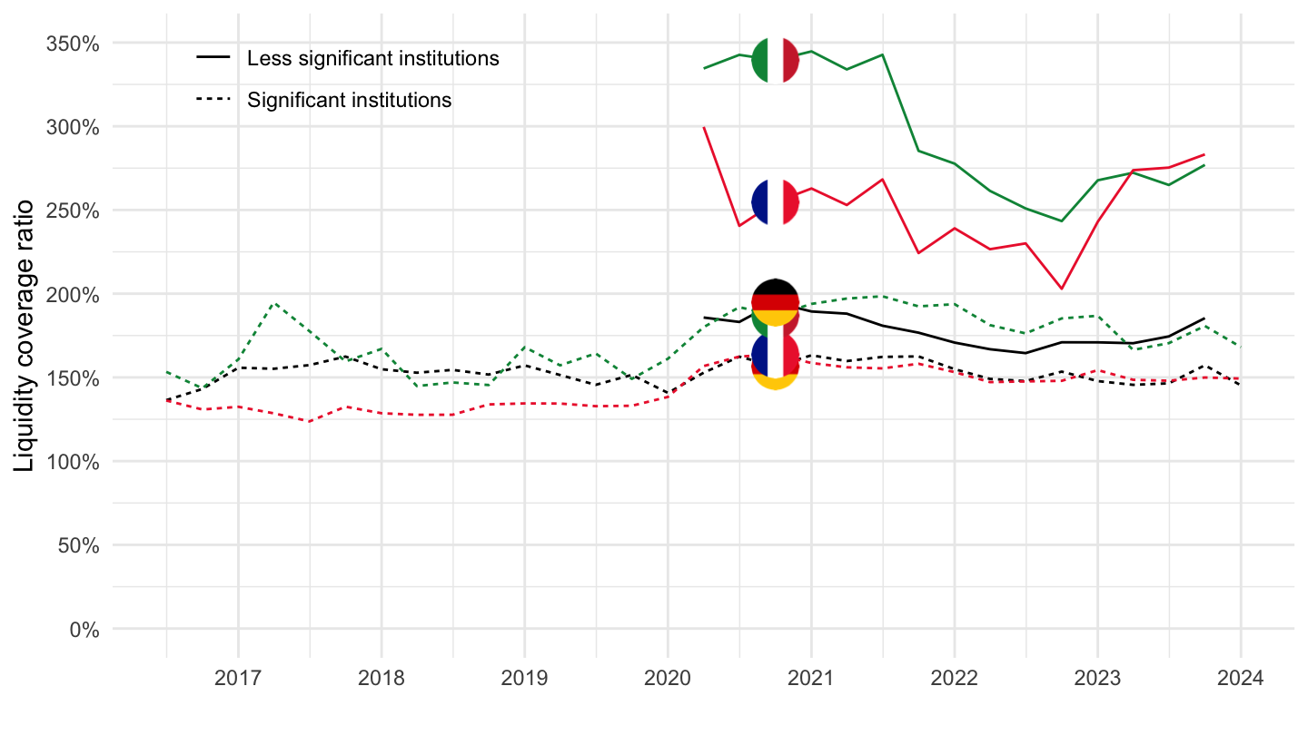

Liquidity buffer

Code

SUP %>%
  filter(CB_ITEM == "A6310",
         REF_AREA %in% c("U2", "FR", "IT", "DE")) %>%
  left_join(REF_AREA, by = "REF_AREA") %>%
  left_join(SBS_DI_1,  by = "SBS_DI_1") %>%
  quarter_to_date %>%
  select_if(~ n_distinct(.) > 1) %>%
  arrange(desc(date)) %>%
  left_join(colors, by = c("Ref_area" = "country")) %>%
  mutate(OBS_VALUE = OBS_VALUE/100) %>%
  ggplot(.) + theme_minimal() + xlab("") + ylab("Liquidity buffer") +
  geom_line(aes(x = date, y = OBS_VALUE, color = color, linetype = Sbs_di_1)) + 
  add_flags(6) + scale_color_identity() +
  scale_x_date(breaks = seq(1960, 2100, 1) %>% paste0("-01-01") %>% as.Date,
               labels = date_format("%Y")) +
  scale_y_continuous(breaks = seq(0, 1000, 2)) +
  theme(legend.position = c(0.2, 0.90),
        legend.title = element_blank())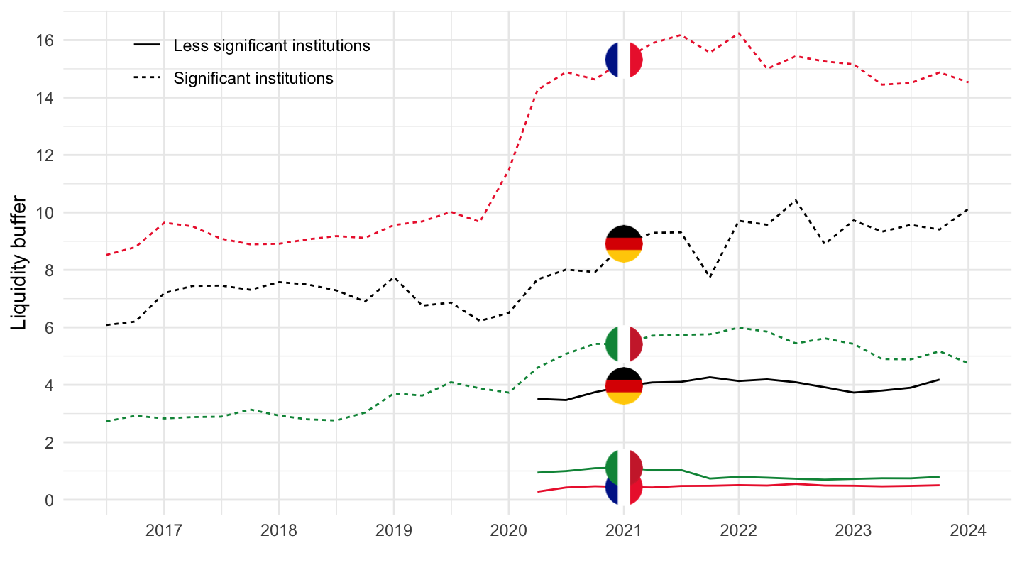

Net liquidity outflow

Code

SUP %>%
  filter(CB_ITEM == "A6320",
         REF_AREA %in% c("U2", "FR", "IT", "DE")) %>%
  left_join(REF_AREA, by = "REF_AREA") %>%
  left_join(SBS_DI_1,  by = "SBS_DI_1") %>%
  quarter_to_date %>%
  select_if(~ n_distinct(.) > 1) %>%
  arrange(desc(date)) %>%
  left_join(colors, by = c("Ref_area" = "country")) %>%
  mutate(OBS_VALUE = OBS_VALUE/100) %>%
  ggplot(.) + theme_minimal() + xlab("") + ylab("Net liquidity outflow") +
  geom_line(aes(x = date, y = OBS_VALUE, color = color, linetype = Sbs_di_1)) + 
  add_flags(6) + scale_color_identity() +
  scale_x_date(breaks = seq(1960, 2100, 1) %>% paste0("-01-01") %>% as.Date,
               labels = date_format("%Y")) +
  scale_y_continuous(breaks = seq(0, 1000, 2)) +
  theme(legend.position = c(0.2, 0.90),
        legend.title = element_blank())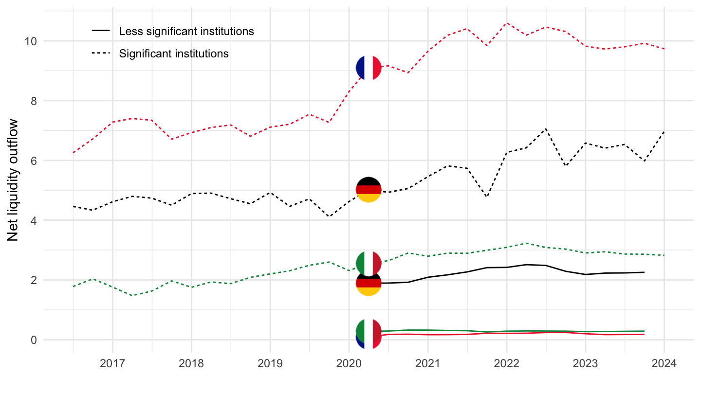

Net liquidity outflow

Code

SUP %>%
  filter(grepl("Net liquidity outflow", TITLE),
         REF_AREA %in% c("B01", "FR", "IT", "DE")) %>%
  left_join(REF_AREA, by = "REF_AREA") %>%
  left_join(SBS_DI_1,  by = "SBS_DI_1") %>%
  quarter_to_date %>%
  mutate(OBS_VALUE = OBS_VALUE/100,
         Ref_area = ifelse(REF_AREA == "B01", "Europe", Ref_area)) %>%
  select_if(~ n_distinct(.) > 1) %>%
  left_join(colors, by = c("Ref_area" = "country")) %>%
  na.omit %>%
  ggplot(.) + theme_minimal() + xlab("") + ylab("Net liquidity outflow") +
  geom_line(aes(x = date, y = OBS_VALUE, color = color, linetype = paste0(SBS_DI_1, SBS_BREAKDOWN))) + 
  add_flags(6) + scale_color_identity() +
  scale_x_date(breaks = seq(1960, 2100, 1) %>% paste0("-01-01") %>% as.Date,
               labels = date_format("%Y")) +
  scale_y_continuous(breaks = 0.01*seq(0, 500, 50),
                     labels = percent_format(accuracy = 1),
                     limits = c(0, 3.5)) +
  theme(legend.position = c(0.55, 0.50),
        legend.title = element_blank())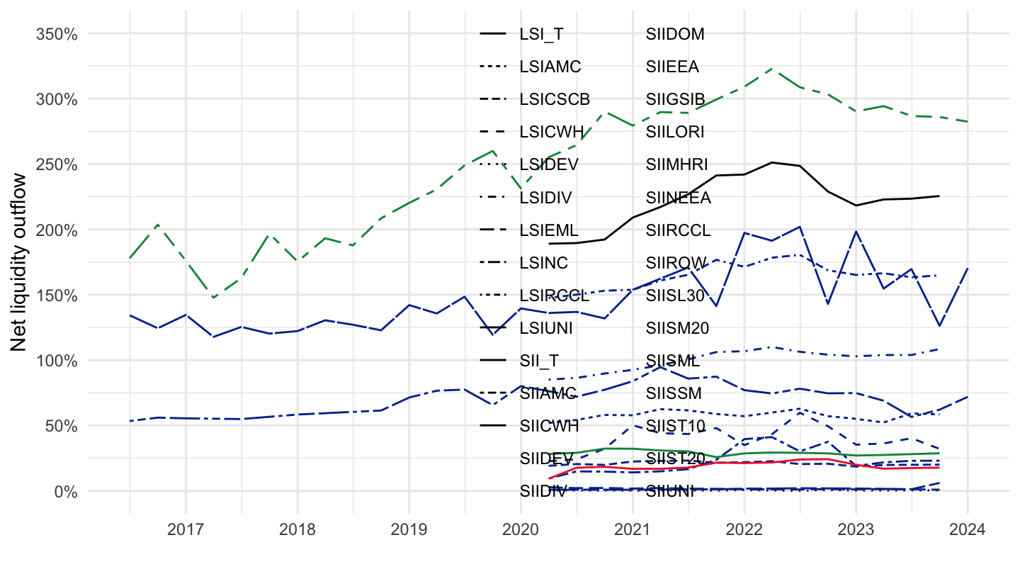

Net Liquidity outflow - EU

B01 - EU countries participating in the Single Supervisory Mechanism (SSM)

Capital adequacy

Common equity Tier 1 ratio
Tier 1 ratio

https://www.bankingsupervision.europa.eu/press/pr/date/2023/html/ssm.pr230111_{4cb4953fd6.en.html#:}:text=The%20aggregate%20capital%20ratios%20of,capital%20ratio%20stood%20at%2018.68%25.