Financial market data - yield curve

Data - ECB

Author

Error in readChar(con, 5L, useBytes = TRUE) : 
  impossible d'ouvrir la connexion

Info

source	dataset	.html	.RData
ecb	YC	2024-06-20	2024-05-21

Data on monetary policy

source	dataset	.html	.RData
bdf	FM	2024-06-30	2024-06-18
bdf	MIR	2024-06-30	2024-06-30
bdf	MIR1	2024-06-30	2024-06-30
bis	CBPOL	2024-06-19	2024-06-07
ecb	BSI	2024-06-30	2024-05-21
ecb	BSI_PUB	2024-06-30	2024-06-30
ecb	FM	2024-06-30	2024-06-30
ecb	ILM	2024-06-30	2024-06-30
ecb	ILM_PUB	2024-06-30	2024-01-25
ecb	liq_daily	2024-06-30	2024-05-21
ecb	MIR	2024-06-19	2024-06-30
ecb	RAI	2024-06-07	2024-06-30
ecb	SUP	2024-06-30	2024-06-30
ecb	YC	2024-06-20	2024-05-21
ecb	YC_PUB	2024-06-30	2024-06-30
eurostat	ei_mfir_m	2024-06-23	2024-06-08
eurostat	irt_st_m	2024-06-23	2024-06-30
fred	r	2024-06-30	2024-06-30
oecd	MEI	2024-04-16	2024-06-30
oecd	MEI_FIN	2024-06-20	2024-05-21

LAST_COMPILE

LAST_COMPILE
2024-07-01

Last

TIME_PERIOD	FREQ	Nobs
2024-05-20	B	2165

INSTRUMENT_FM

Code

YC %>%
  left_join(INSTRUMENT_FM,  by = "INSTRUMENT_FM") %>%
  group_by(INSTRUMENT_FM, Instrument_fm) %>%
  summarise(Nobs = n()) %>%
  arrange(-Nobs) %>%
  print_table_conditional

INSTRUMENT_FM	Instrument_fm	Nobs
G_N_A	Government bond, nominal, all issuers whose rating is triple A	5455429
G_N_C	Government bond, nominal, all issuers all ratings included	5439960
G_N_W	Government bond, nominal, all issuers whose rating is between AAA and AA	7346

DATA_TYPE_FM

Code

YC %>%
  left_join(DATA_TYPE_FM,  by = "DATA_TYPE_FM") %>%
  group_by(DATA_TYPE_FM, Data_type_fm) %>%
  summarise(Nobs = n()) %>%
  arrange(-Nobs) %>%
  print_table_conditional

TIME_PERIOD

Code

YC %>%
  group_by(TIME_PERIOD) %>%
  summarise(Nobs = n()) %>%
  arrange(desc(TIME_PERIOD)) %>%
  print_table_conditional()

Yield curve

Government bond, nominal, all issuers whose rating is triple A

Linear

Code

YC %>%
  filter(DATA_TYPE_FM %in% paste0("PY_", 1:30, "Y"),
         INSTRUMENT_FM == "G_N_C") %>%
  filter(TIME_PERIOD %in% c(as.Date(c("2022-11-01", "2022-03-01")), max(TIME_PERIOD))) %>%
  mutate(year = parse_number(DATA_TYPE_FM)) %>%
  ggplot + geom_line(aes(x = year, y = OBS_VALUE/100, color = paste0(TIME_PERIOD))) +
  theme_minimal() + xlab("Maturity in rates") + ylab("Par yield curve rate") +
  scale_x_continuous(breaks = c(1, 2, 5, 10, 15, 20, 25, 30),
                     labels = dollar_format(accuracy = 1, pre = "", su = "Y")) +
  scale_y_continuous(breaks = 0.01*seq(-10, 50, 0.5),
                     labels = percent_format(accuracy = .1)) +
  theme(legend.position = c(0.9, 0.2),
        legend.title = element_blank())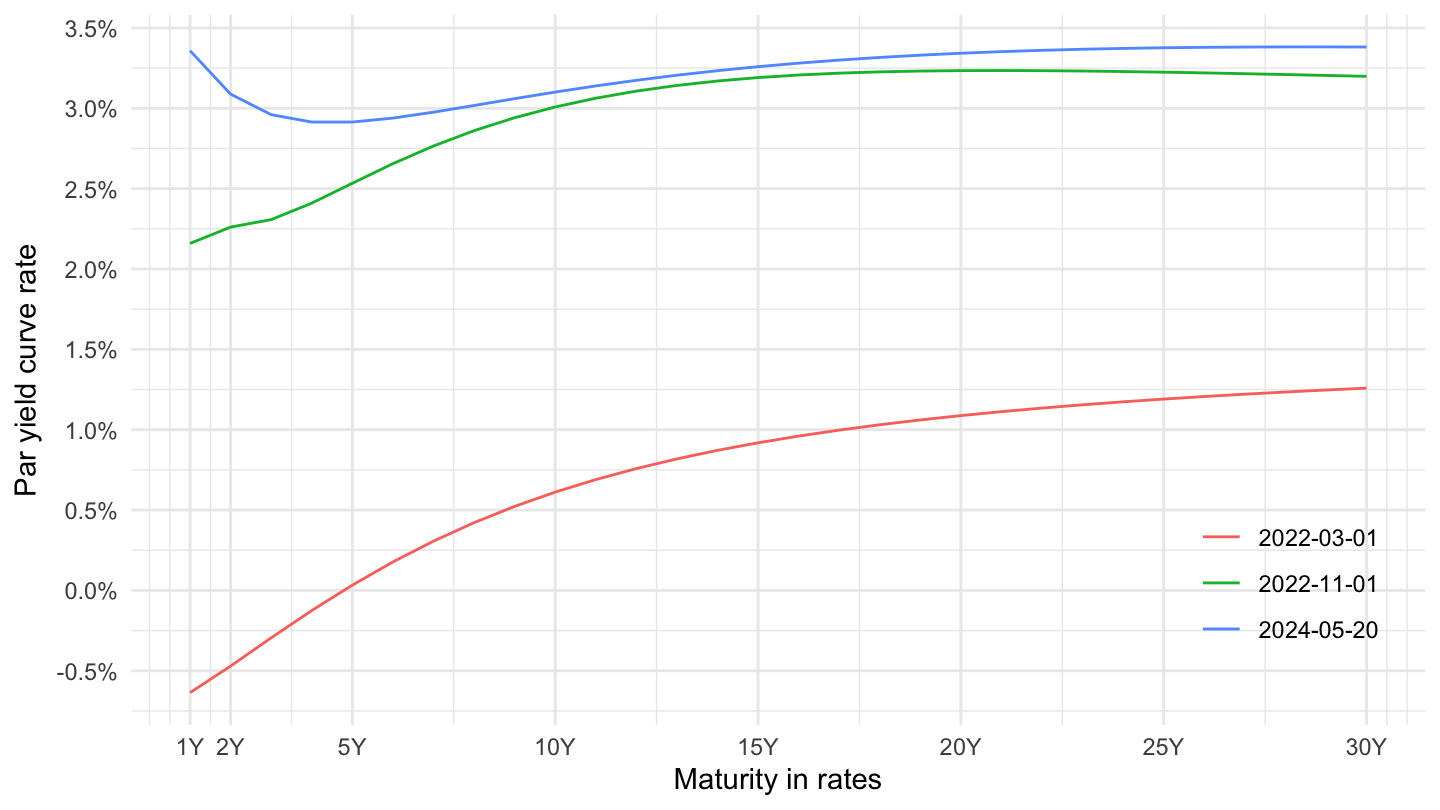

Log

Code

YC %>%
  filter(DATA_TYPE_FM %in% paste0("PY_", 1:30, "Y"),
         INSTRUMENT_FM == "G_N_C") %>%
  filter(TIME_PERIOD %in% c(as.Date(c("2023-03-01", "2022-11-03", "2022-07-01", "2022-03-01")), max(TIME_PERIOD))) %>%
  mutate(year = parse_number(DATA_TYPE_FM)) %>%
  ggplot + geom_line(aes(x = year, y = OBS_VALUE/100, color = paste0(TIME_PERIOD))) +
  theme_minimal() + xlab("Maturity in rates") + ylab("Par yield curve rate") +
  scale_x_log10(breaks = c(1, 2, 5, 10, 15, 20, 25, 30),
                     labels = dollar_format(accuracy = 1, pre = "", su = "Y")) +
  scale_y_continuous(breaks = 0.01*seq(-10, 50, 0.5),
                     labels = percent_format(accuracy = .1)) +
  theme(legend.position = c(0.9, 0.2),
        legend.title = element_blank())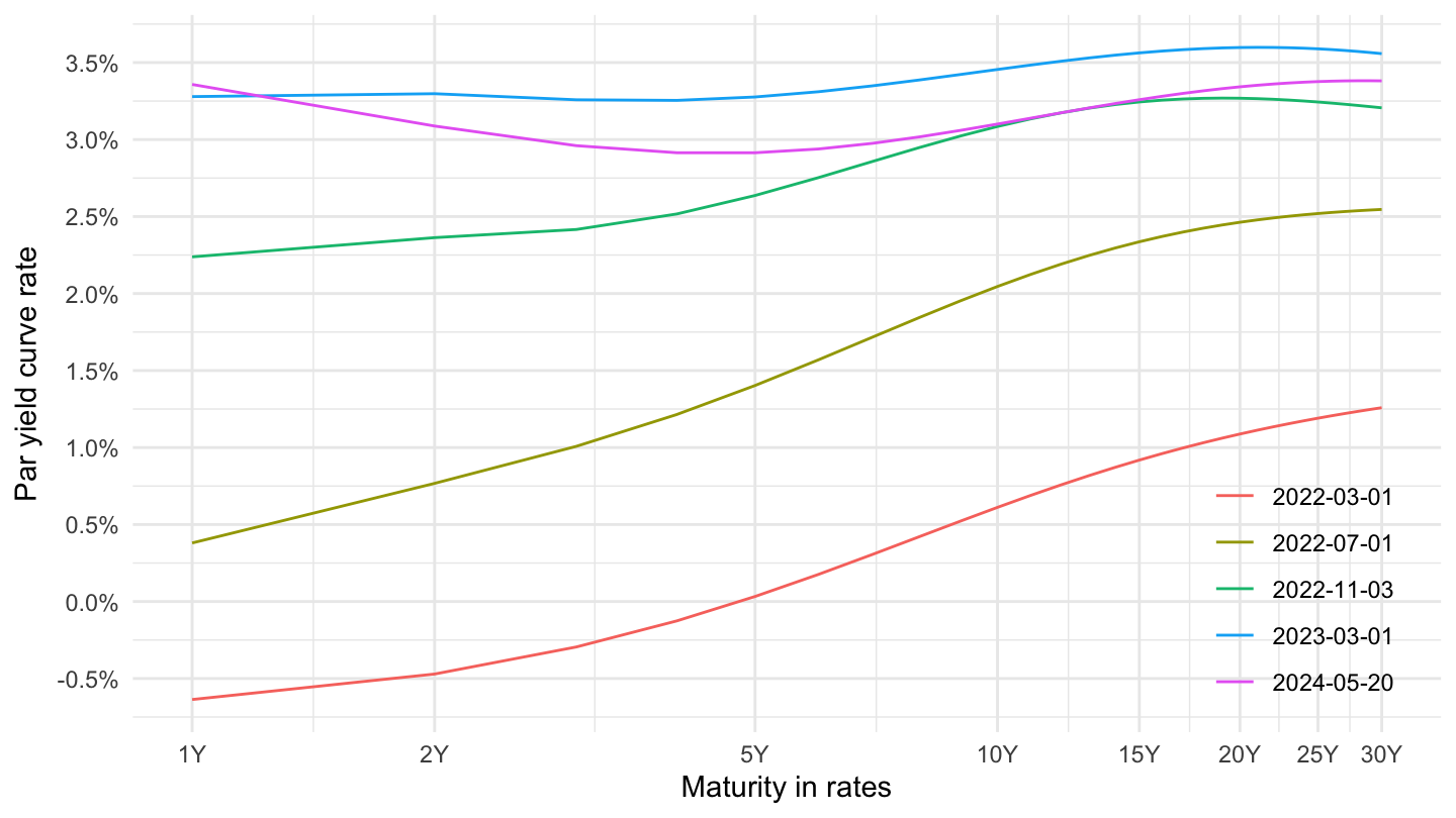

Log2

Code

YC %>%
  filter(DATA_TYPE_FM %in% c(paste0("PY_", 1:30, "Y"), paste0("PY_", 1:12, "M")),
         INSTRUMENT_FM == "G_N_C") %>%
  filter(TIME_PERIOD %in% c(as.Date(c("2022-11-03", "2022-07-01", "2022-03-01", "2021-11-01")), max(TIME_PERIOD))) %>%
  mutate(number = parse_number(DATA_TYPE_FM),
         number = ifelse(DATA_TYPE_FM %in% paste0("PY_", 1:12, "M"), number/12, number)) %>%
  ggplot + geom_line(aes(x = number, y = OBS_VALUE/100, color = paste0(TIME_PERIOD))) +
  theme_minimal() + xlab("Maturity") + ylab("Par yield curve rate") +
  scale_x_log10(breaks = c(1/12, 3/12, 6/12, 9/12, 1, 2, 5, 10, 15, 20, 30),
                     labels = c("1M", "3M", "6M", "9M", "1Y", "2Y", "5Y", "10Y", "15Y", "20Y", "30Y")) +
  scale_y_continuous(breaks = 0.01*seq(-10, 50, 0.5),
                     labels = percent_format(accuracy = .1)) +
  theme(legend.position = c(0.9, 0.2),
        legend.title = element_blank())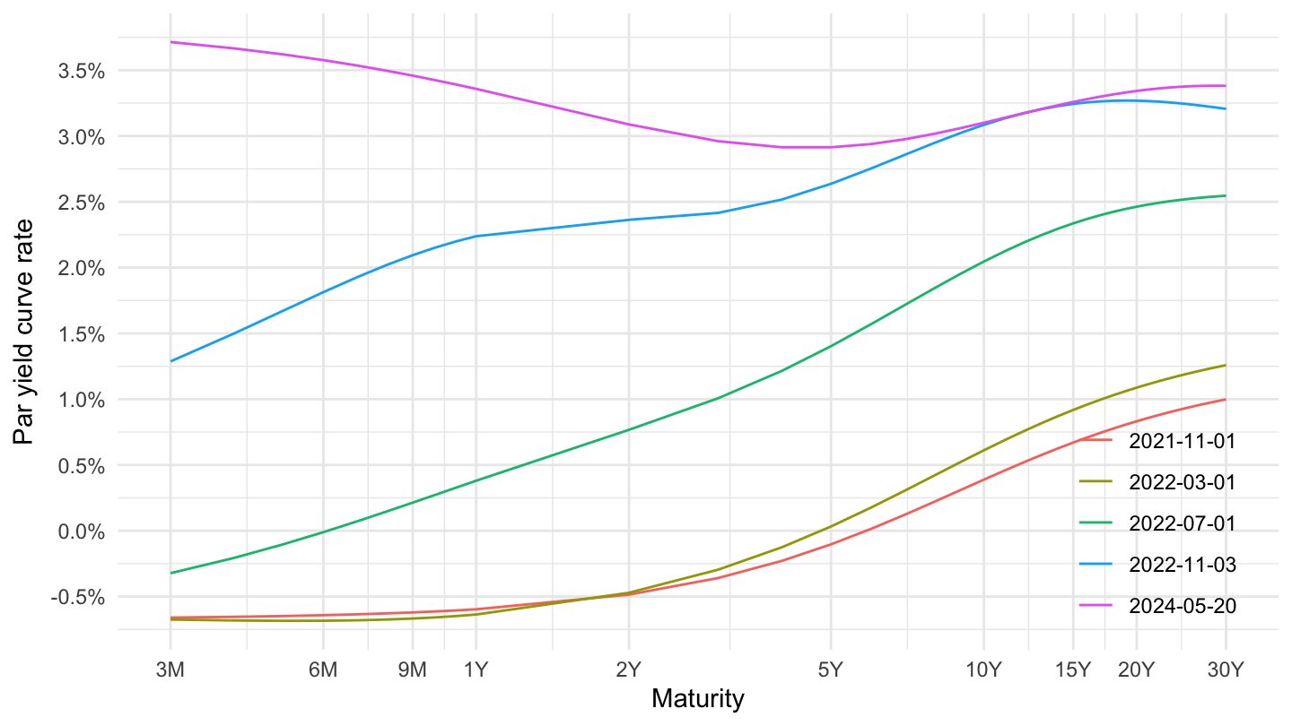

Log2

Code

YC %>%
  filter(DATA_TYPE_FM %in% c(paste0("PY_", 1:30, "Y"), paste0("PY_", 1:12, "M"))) %>%
  filter(TIME_PERIOD %in% c(as.Date(c("2022-11-03", "2022-07-01", "2022-03-01", "2021-11-01")), max(TIME_PERIOD))) %>%
  mutate(number = parse_number(DATA_TYPE_FM),
         number = ifelse(DATA_TYPE_FM %in% paste0("PY_", 1:12, "M"), number/12, number)) %>%
  left_join(INSTRUMENT_FM,  by = "INSTRUMENT_FM") %>%
  ggplot + geom_line(aes(x = number, y = OBS_VALUE/100, color = paste0(TIME_PERIOD), linetype = Instrument_fm)) +
  theme_minimal() + xlab("Maturity") + ylab("Par yield curve rate") +
  scale_x_log10(breaks = c(1/12, 3/12, 6/12, 9/12, 1, 2, 5, 10, 15, 20, 30),
                     labels = c("1M", "3M", "6M", "9M", "1Y", "2Y", "5Y", "10Y", "15Y", "20Y", "30Y")) +
  scale_y_continuous(breaks = 0.01*seq(-10, 50, 0.5),
                     labels = percent_format(accuracy = .1)) +
  theme(legend.position = c(0.4, 0.4),
        legend.title = element_blank())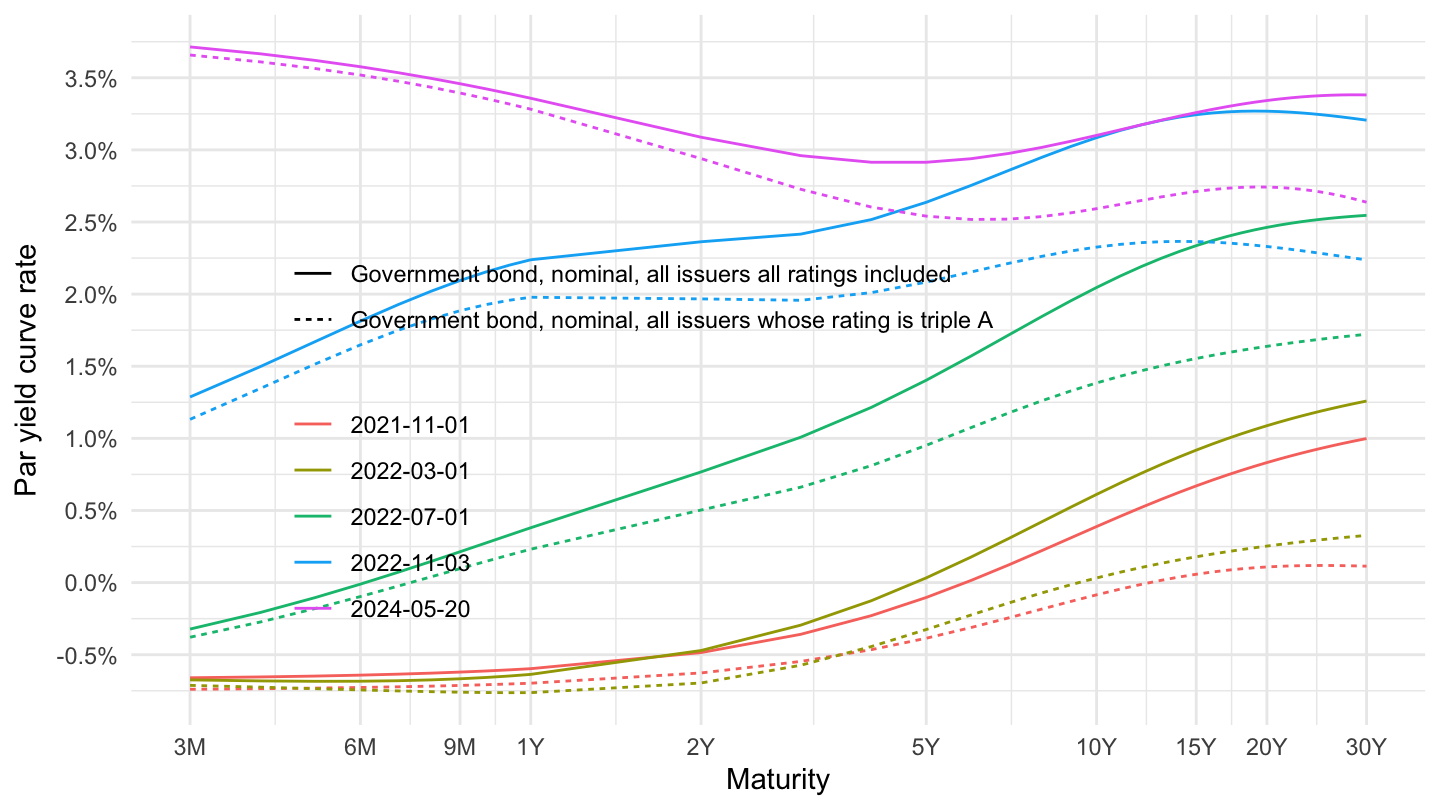

Yield curve

2 years

Code

YC %>%
  filter(DATA_TYPE_FM == "PY_2Y") %>%
  select_if(~ n_distinct(.) > 1) %>%
  day_to_date %>%
  arrange(desc(date)) %>%
  left_join(INSTRUMENT_FM,  by = "INSTRUMENT_FM") %>%
  ggplot + geom_line(aes(x = date, y = OBS_VALUE/100, color = Instrument_fm)) +
  theme_minimal() + xlab("") + ylab("2-year rates") +
  scale_x_date(breaks = seq(1960, 2024, 2) %>% paste0("-01-01") %>% as.Date,
               labels = date_format("%Y")) +
  scale_y_continuous(breaks = 0.01*seq(-10, 50, 0.5),
                     labels = percent_format(accuracy = .1)) +
  theme(legend.position = c(0.6, 0.9),
        legend.title = element_blank())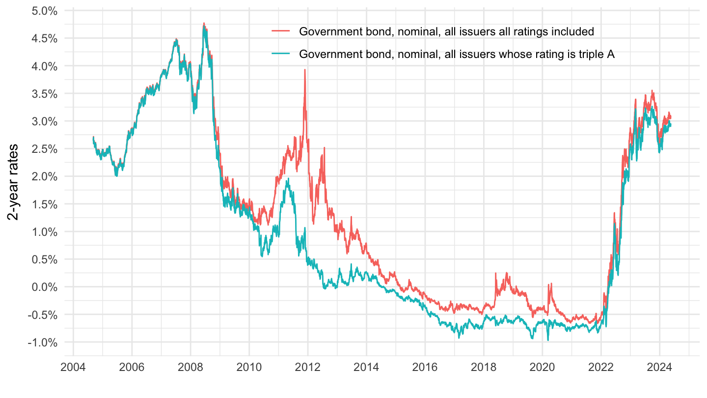

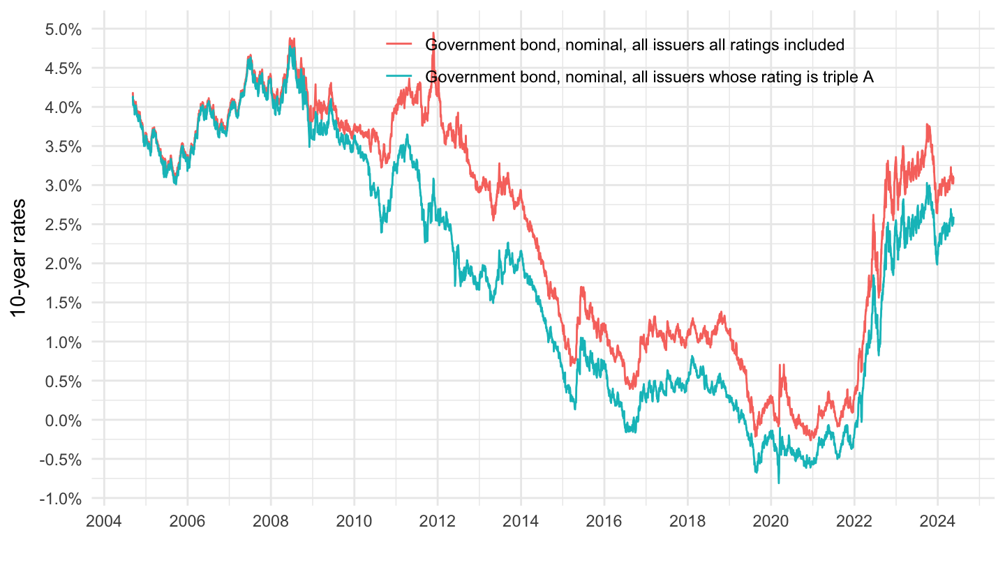
10 years

Code

YC %>%
  filter(DATA_TYPE_FM == "PY_10Y") %>%
  select_if(~ n_distinct(.) > 1) %>%
  day_to_date %>%
  arrange(desc(date)) %>%
  left_join(INSTRUMENT_FM,  by = "INSTRUMENT_FM") %>%
  ggplot + geom_line(aes(x = date, y = OBS_VALUE/100, color = Instrument_fm)) +
  theme_minimal() + xlab("") + ylab("10-year rates") +
  scale_x_date(breaks = seq(1960, 2024, 2) %>% paste0("-01-01") %>% as.Date,
               labels = date_format("%Y")) +
  scale_y_continuous(breaks = 0.01*seq(-10, 50, 0.5),
                     labels = percent_format(accuracy = .1)) +
  theme(legend.position = c(0.6, 0.9),
        legend.title = element_blank())