Main Economic Indicators - MEI

Data - OECD

Author

François Geerolf

Last observation: Q1 2024 (N = 62) · janv. 2024 (N = 1629) · 2023 (N = 11067)

First observation: Q4 1955 (N = 1) · 1960 (N = 2679) · janv. 1960 (N = 1834)

Last data update: 02 août 2026, 09:01

Last compile: 02 sept. 2026, 23:34

Structure

Nobs - Javascript

Code

MEI |>
  left_join(MEI_var$SUBJECT, by = c("SUBJECT")) %>%
  {if (!is_html_output()) mutate(., Subject = substr(Subject, 1, 87)) else .} |>
  group_by(SUBJECT, Subject, MEASURE, FREQUENCY) |>
  filter(!is.na(obsValue)) |>
  summarise(Nobs = n()) |>
  arrange(-Nobs) %>%
  {if (is_html_output()) datatable(., filter = 'top', rownames = F) else .}

Monetary Base

M1

All

Code

MEI |>
  filter(LOCATION %in% c("FRA", "USA", "JPN", "DEU"),
         SUBJECT == "MANMM101",
         MEASURE == "IXOB",
         FREQUENCY == "M") |>
  month_to_date() |>
  #filter(date >= as.Date("1990-01-01")) %>%
  left_join(MEI_var$LOCATION, by = "LOCATION") |>
  add_flag_color("Location") |>
  group_by(LOCATION) |>
  mutate(obsValue = obsValue/obsValue[1]) |>
  ggplot() + geom_line(aes(x = date, y = obsValue, color = color)) + 
  scale_color_identity() + add_2flags + theme_minimal() + xlab("") + ylab("M1") +
  scale_x_date(breaks = seq(1960, 2100, 5) |> paste0("-01-01") |> as.Date(),
               labels = date_format("%Y")) +
  scale_y_log10(breaks = c(seq(1, 50, 1), 100, 150, 200, 500, 1000))

1990-

Code

MEI |>
  filter(LOCATION %in% c("FRA", "USA", "JPN", "DEU"),
         SUBJECT == "MANMM101",
         MEASURE == "IXOB",
         FREQUENCY == "M") |>
  month_to_date() |>
  filter(date >= as.Date("1990-01-01")) |>
  left_join(MEI_var$LOCATION, by = "LOCATION") |>
  add_flag_color("Location") |>
  group_by(LOCATION) |>
  mutate(obsValue = obsValue/obsValue[1]) |>
  ggplot() + geom_line(aes(x = date, y = obsValue, color = color)) + 
  scale_color_identity() + add_2flags + theme_minimal() + xlab("") + ylab("M1") +
  scale_x_date(breaks = seq(1960, 2100, 5) |> paste0("-01-01") |> as.Date(),
               labels = date_format("%Y")) +
  scale_y_log10(breaks = c(seq(1, 50, 1), 100, 150, 200, 500, 1000))

M3

All

Code

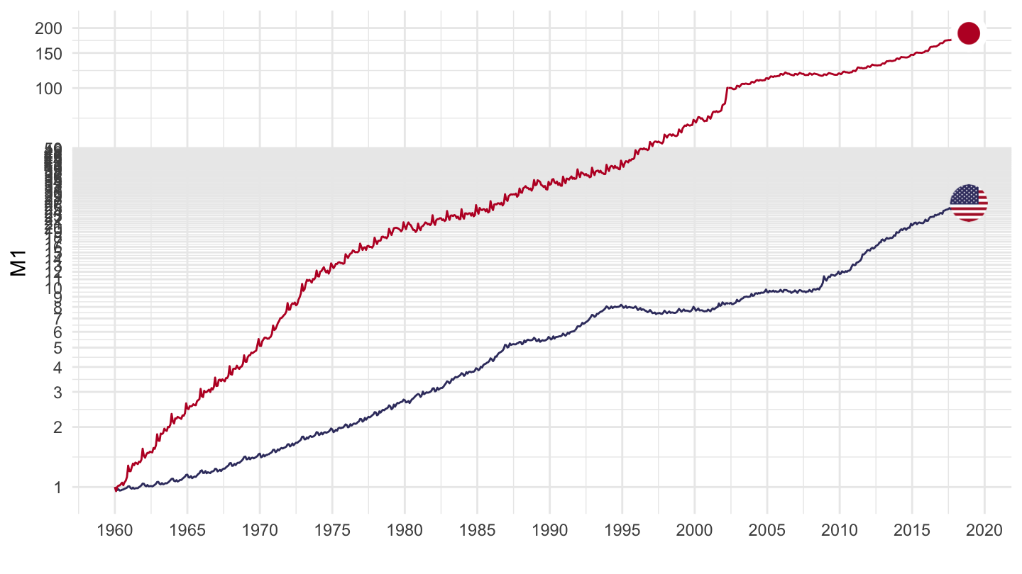
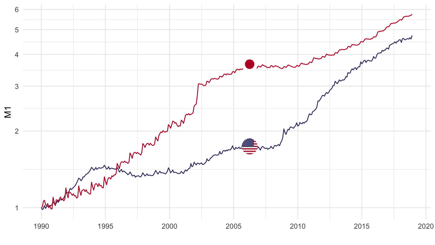
MEI |>
  filter(LOCATION %in% c("FRA", "USA", "JPN", "DEU"),
         SUBJECT == "MABMM301",
         MEASURE == "IXOB",
         FREQUENCY == "M") |>
  month_to_date() |>
  left_join(MEI_var$LOCATION, by = "LOCATION") |>
  add_flag_color("Location") |>
  group_by(LOCATION) |>
  mutate(obsValue = obsValue/obsValue[1]) |>
  ggplot() + geom_line(aes(x = date, y = obsValue, color = color)) + 
  scale_color_identity() + add_2flags + theme_minimal() + xlab("") + ylab("M3") +
  scale_x_date(breaks = seq(1960, 2100, 5) |> paste0("-01-01") |> as.Date(),
               labels = date_format("%Y")) +
  scale_y_log10(breaks = c(seq(1, 50, 1), 100, 150, 200, 500, 1000))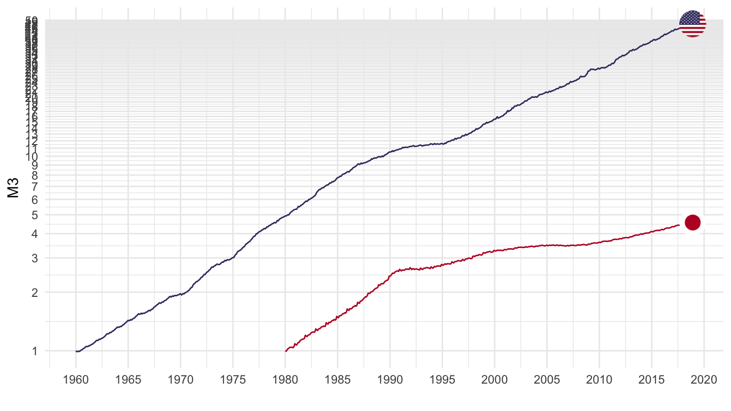

1990-

Code

MEI |>
  filter(LOCATION %in% c("FRA", "USA", "JPN", "DEU"),
         SUBJECT == "MABMM301",
         MEASURE == "IXOB",
         FREQUENCY == "M") |>
  month_to_date() |>
  filter(date >= as.Date("1990-01-01")) |>
  left_join(MEI_var$LOCATION, by = "LOCATION") |>
  add_flag_color("Location") |>
  group_by(LOCATION) |>
  mutate(obsValue = obsValue/obsValue[1]) |>
  ggplot() + geom_line(aes(x = date, y = obsValue, color = color)) + 
  scale_color_identity() + add_2flags + theme_minimal() + xlab("") + ylab("M3") +
  scale_x_date(breaks = seq(1960, 2100, 5) |> paste0("-01-01") |> as.Date(),
               labels = date_format("%Y")) +
  scale_y_log10(breaks = c(seq(1, 50, 1), 100, 150, 200, 500, 1000))

M1 and M3

LT Interest Rates

France, Germany, Japan

Code

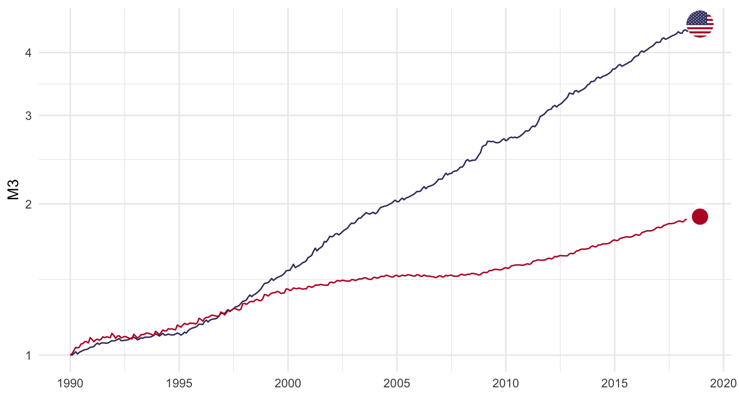
MEI |>
  filter(LOCATION %in% c("FRA", "DEU", "JPN"),
         SUBJECT == "IRLTLT01",
         FREQUENCY == "M") |>
  month_to_date() |>
  filter(date >= as.Date("2010-01-01")) |>
  left_join(MEI_var$LOCATION, by = "LOCATION") |>
  add_flag_color("Location") |>
  mutate(obsValue = obsValue / 100) |>
  ggplot() + geom_line(aes(x = date, y = obsValue, color = color)) + 
  scale_color_identity() +
  theme_minimal() + xlab("") + ylab("Long-Term Interest Rates (%)") +
  add_3flags +
  scale_x_date(breaks = seq(1960, 2100, 1) |> paste0("-01-01") |> as.Date(),
               labels = date_format("%Y")) +
  scale_y_continuous(breaks = 0.01*seq(-10, 50, 1),
                     labels = percent_format(accuracy = 1)) +
  theme(legend.position = "none") +
  geom_hline(yintercept = 0, linetype = "dashed")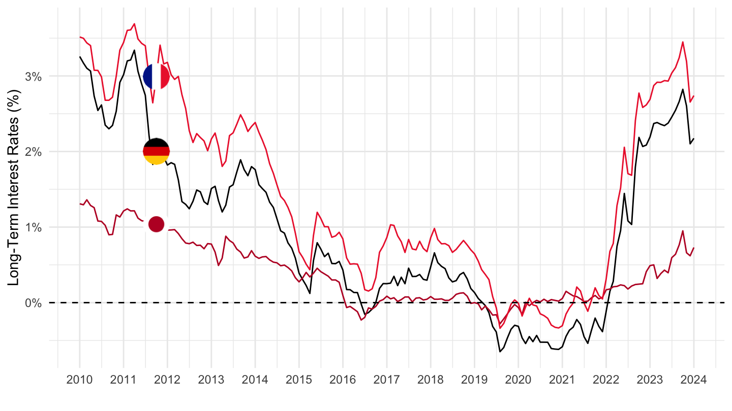

2019-2021

Code

MEI |>
  filter(LOCATION %in% c("FRA", "DEU", "JPN"),
         SUBJECT == "IRLTLT01",
         FREQUENCY == "M") |>
  month_to_date() |>
  filter(date >= as.Date("2014-02-01")) |>
  left_join(MEI_var$LOCATION, by = "LOCATION") |>
  group_by(LOCATION) |>
  mutate(obsValue = obsValue / 100) |>
  ggplot() + geom_line(aes(x = date, y = obsValue, color = Location)) + 
  theme_minimal() + xlab("") + ylab("Taux Nominal sur la Dette, 10 ans (%)") +
  add_3flags +
  scale_x_date(breaks = "1 year",
               labels = date_format("%Y")) +
  scale_y_continuous(breaks = 0.01*seq(-10, 50, .2),
                     labels = percent_format(accuracy = .1)) +
  scale_color_manual(values = c("#002395", "#000000", "#BC002D")) +
  theme(legend.position = "none") +
  geom_hline(yintercept = 0, linetype = "dashed")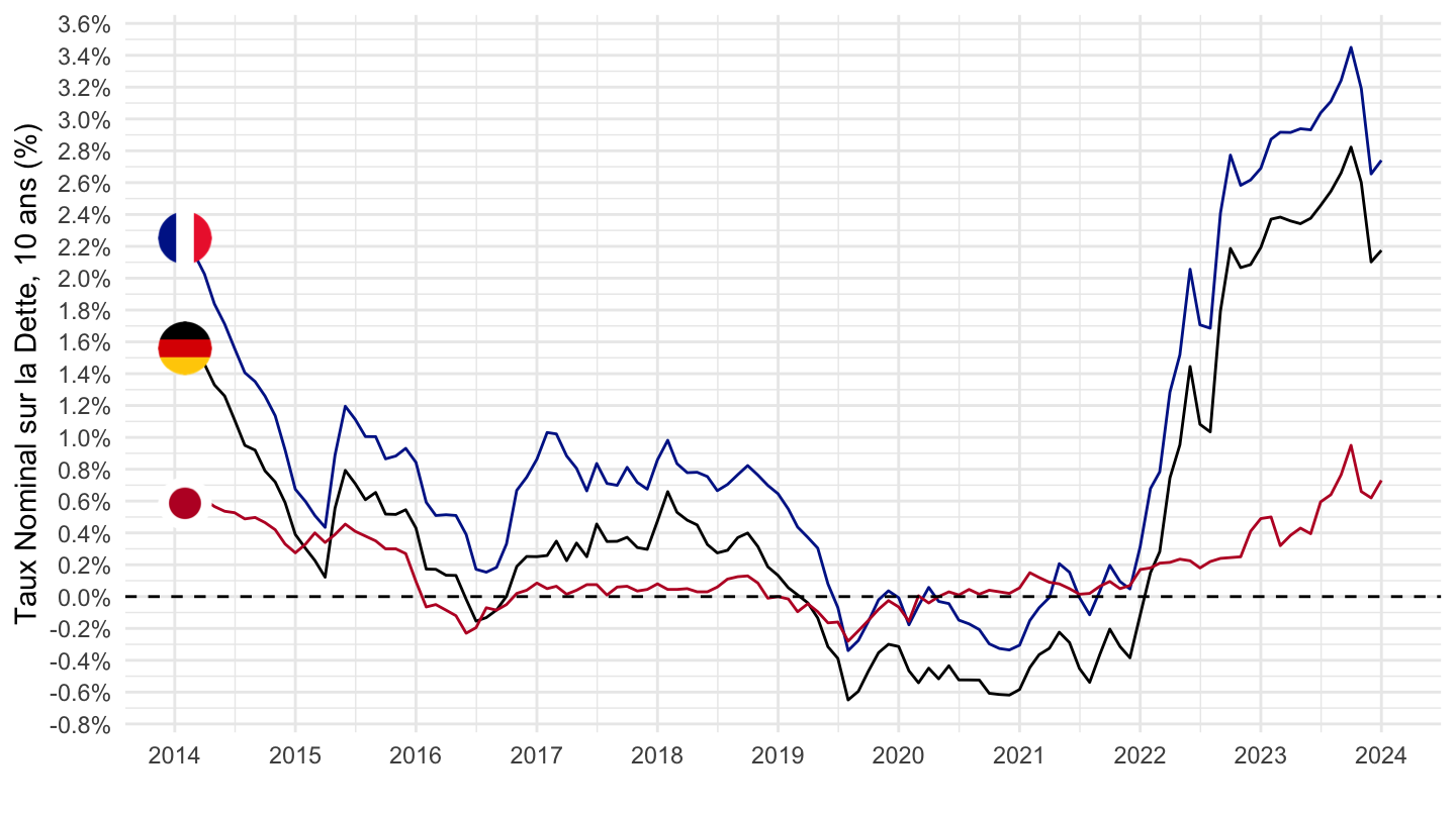

France, United States, Germany, Japan

All

Code

MEI |>
  filter(LOCATION %in% c("FRA", "USA", "DEU", "JPN"),
         SUBJECT == "IRLTLT01",
         FREQUENCY == "M") |>
  month_to_date() |>
  left_join(MEI_var$LOCATION, by = "LOCATION") |>
  add_flag_color("Location") |>
  group_by(LOCATION) |>
  mutate(obsValue = obsValue / 100) |>
  ggplot() + geom_line(aes(x = date, y = obsValue, color = color)) + 
  add_4flags +
  theme_minimal() + xlab("") + ylab("Long-Term Interest Rates (%)") +
  scale_x_date(breaks = seq(1960, 2100, 5) |> paste0("-01-01") |> as.Date(),
               labels = date_format("%Y")) +
  scale_y_continuous(breaks = 0.01*seq(-10, 50, 1),
                     labels = percent_format(accuracy = 1)) +
  theme(legend.position = c(0.8, 0.80),
        legend.title = element_blank()) +
  scale_color_identity()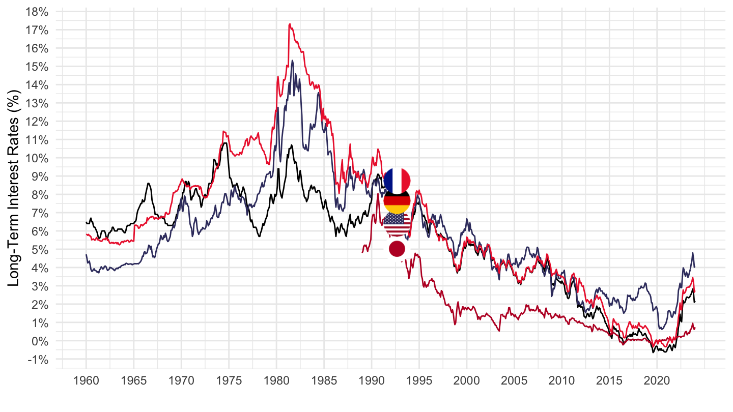

1990-

Code

MEI |>
  filter(LOCATION %in% c("FRA", "USA", "DEU", "JPN"),
         SUBJECT == "IRLTLT01",
         FREQUENCY == "M") |>
  month_to_date() |>
  filter(date >= as.Date("1990-01-01")) |>
  left_join(MEI_var$LOCATION, by = "LOCATION") |>
  add_flag_color("Location") |>
  group_by(LOCATION) |>
  mutate(obsValue = obsValue / 100) |>
  ggplot() + geom_line(aes(x = date, y = obsValue, color = color)) + 
  scale_color_identity() + add_4flags +
  theme_minimal() + xlab("") + ylab("Long-Term Interest Rates (%)") +
  scale_x_date(breaks = seq(1960, 2100, 5) |> paste0("-01-01") |> as.Date(),
               labels = date_format("%Y")) +
  scale_y_continuous(breaks = 0.01*seq(-10, 50, 1),
                     labels = percent_format(accuracy = 1)) +
  theme(legend.position = c(0.8, 0.80),
        legend.title = element_blank())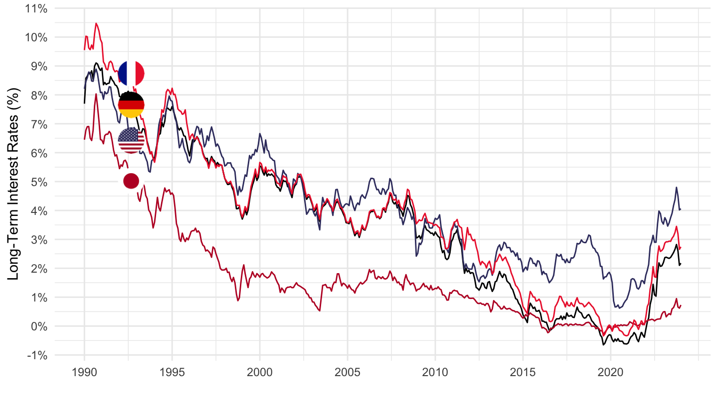

2010-

Code

MEI |>
  filter(LOCATION %in% c("FRA", "USA", "DEU", "JPN"),
         SUBJECT == "IRLTLT01",
         FREQUENCY == "M") |>
  month_to_date() |>
  filter(date >= as.Date("2010-01-01")) |>
  left_join(MEI_var$LOCATION, by = "LOCATION") |>
  add_flag_color("Location") |>
  group_by(LOCATION) |>
  ggplot() + geom_line(aes(x = date, y = obsValue / 100, color = color)) + 
  theme_minimal() + xlab("") + ylab("Long-Term Interest Rates (%)") +
  geom_image(data = . %>%
               filter(date == as.Date("2014-01-01")) %>%
               mutate(image = paste0("../../icon/flag/round/", str_to_lower(gsub(" ", "-", Location)), ".png")),
             aes(x = date, y = obsValue / 100, image = image), asp = 1.5) +
  scale_x_date(breaks = seq(1960, 2100, 1) |> paste0("-01-01") |> as.Date(),
               labels = date_format("%Y")) +
  scale_y_continuous(breaks = 0.01*seq(-10, 50, 1),
                     labels = percent_format(accuracy = 1)) +
  theme(legend.position = "none") +
  scale_color_identity()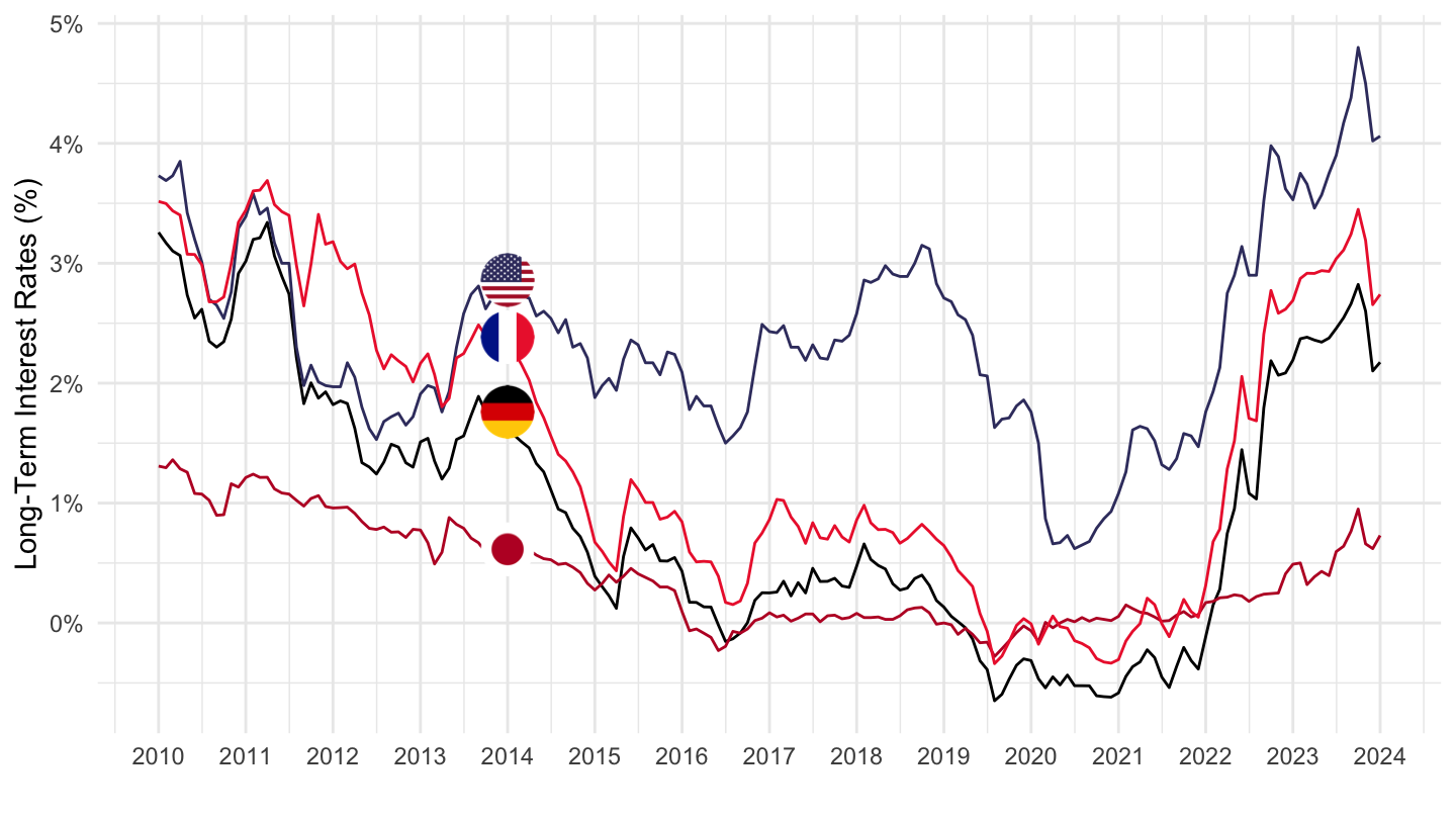

Employment Rates

United States

2000-

Code

MEI |>
  filter(LOCATION %in% c("USA"),
         SUBJECT %in% c("LREM24TT", "LREM55TT", "LREM25TT", "LREM64TT", "LREMTTTT"),
         FREQUENCY == "Q",
         MEASURE == "STSA") |>
  quarter_to_date() |>
  left_join(MEI_var$LOCATION, by = "LOCATION") |>
  left_join(MEI_var$SUBJECT, by = "SUBJECT") |>
  mutate(obsValue = obsValue / 100,
         Subject = gsub("Labour Force Survey - quarterly rates > Employment rate > Aged ", "", Subject),
         Subject = gsub(" > All persons", "", Subject)) |>
  filter(date >= as.Date("2000-01-01")) |>
  ggplot() + geom_line(aes(x = date, y = obsValue, color = Subject)) + 
  scale_y_continuous(breaks = 0.01*seq(-10, 100, 5),
                     labels = percent_format(accuracy = 1)) +
  theme_minimal() + xlab("") + ylab("Employment Rates (%)") +
  scale_x_date(breaks = seq(1960, 2100, 1) |> paste0("-01-01") |> as.Date(),
               labels = date_format("%Y")) +
  theme(legend.position = c(0.4, 0.80),
        legend.title = element_blank(),
        legend.direction = "horizontal")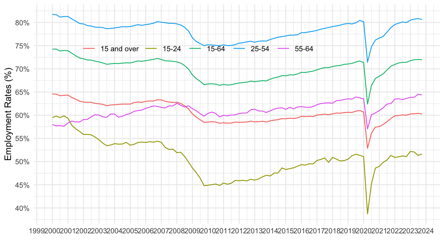

2007-

Code

MEI |>
  filter(LOCATION %in% c("USA"),
         SUBJECT %in% c("LREM24TT", "LREM55TT", "LREM25TT", "LREM64TT", "LREMTTTT"),
         FREQUENCY == "Q",
         MEASURE == "STSA") |>
  quarter_to_date() |>
  left_join(MEI_var$LOCATION, by = "LOCATION") |>
  left_join(MEI_var$SUBJECT, by = "SUBJECT") |>
  mutate(obsValue = obsValue / 100,
         Subject = gsub("Labour Force Survey - quarterly rates > Employment rate > Aged ", "", Subject),
         Subject = gsub(" > All persons", "", Subject)) |>
  filter(date >= as.Date("2007-01-01")) |>
  ggplot() + geom_line(aes(x = date, y = obsValue, color = Subject)) + 
  scale_y_continuous(breaks = 0.01*seq(-10, 100, 5),
                     labels = percent_format(accuracy = 1)) +
  theme_minimal() + xlab("") + ylab("Employment Rates (%)") +
  scale_x_date(breaks = seq(1960, 2100, 1) |> paste0("-01-01") |> as.Date(),
               labels = date_format("%Y")) +
  theme(legend.position = c(0.4, 0.80),
        legend.title = element_blank(),
        legend.direction = "horizontal")

France

All

Code

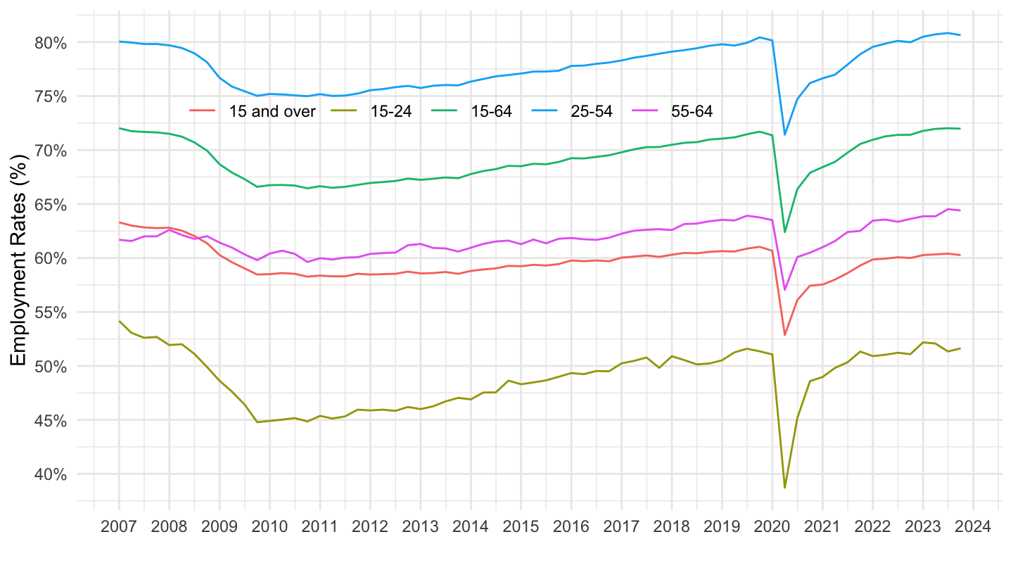
MEI |>
  filter(LOCATION %in% c("FRA"),
         SUBJECT %in% c("LREM24TT", "LREM55TT", "LREM25TT", "LREM64TT", "LREMTTTT"),
         FREQUENCY == "Q",
         MEASURE == "STSA") |>
  quarter_to_date() |>
  left_join(MEI_var$LOCATION, by = "LOCATION") |>
  left_join(MEI_var$SUBJECT, by = "SUBJECT") |>
  mutate(obsValue = obsValue / 100,
         Subject = gsub("Labour Force Survey - quarterly rates > Employment rate > Aged ", "", Subject),
         Subject = gsub(" > All persons", "", Subject)) |>
  filter(date >= as.Date("2007-01-01")) |>
  ggplot() + geom_line(aes(x = date, y = obsValue, color = Subject)) + 
  scale_y_continuous(breaks = 0.01*seq(-10, 100, 5),
                     labels = percent_format(accuracy = 1)) +
  theme_minimal() + xlab("") + ylab("Employment Rates (%)") +
  scale_x_date(breaks = seq(1960, 2100, 1) |> paste0("-01-01") |> as.Date(),
               labels = date_format("%Y")) +
  theme(legend.position = c(0.4, 0.80),
        legend.title = element_blank(),
        legend.direction = "horizontal")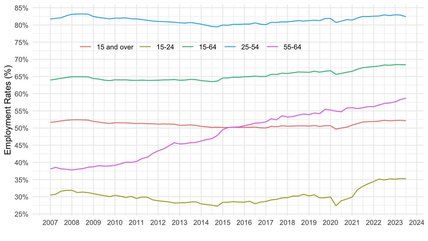

Males

Code

MEI |>
  filter(LOCATION %in% c("FRA"),
         SUBJECT %in% c("LREM24MA", "LREM55MA", "LREM25MA", "LREM64MA", "LREMTTMA"),
         FREQUENCY == "Q",
         MEASURE == "STSA") |>
  quarter_to_date() |>
  left_join(MEI_var$LOCATION, by = "LOCATION") |>
  left_join(MEI_var$SUBJECT, by = "SUBJECT") |>
  mutate(obsValue = obsValue / 100,
         Subject = gsub("Labour Force Survey - quarterly rates > Employment rate > Aged ", "", Subject),
         Subject = gsub(" > Males", "", Subject)) |>
  filter(date >= as.Date("2007-01-01")) |>
  ggplot() + geom_line(aes(x = date, y = obsValue, color = Subject)) + 
  scale_y_continuous(breaks = 0.01*seq(-10, 100, 5),
                     labels = percent_format(accuracy = 1)) +
  theme_minimal() + xlab("") + ylab("Male Employment Rates (%)") +
  scale_x_date(breaks = seq(1960, 2100, 1) |> paste0("-01-01") |> as.Date(),
               labels = date_format("%Y")) +
  theme(legend.position = c(0.4, 0.80),
        legend.title = element_blank(),
        legend.direction = "horizontal")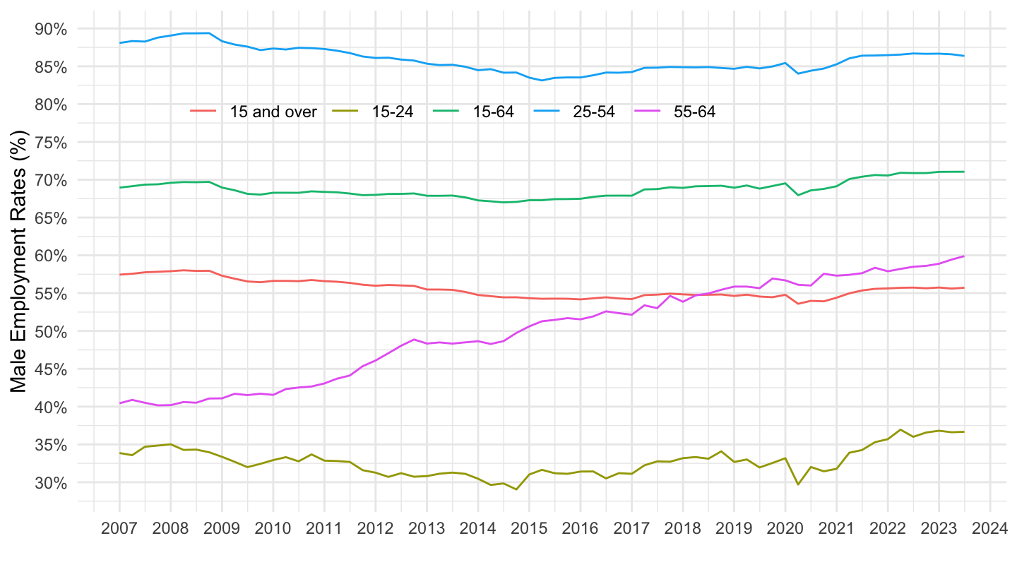

Females

Code

MEI |>
  filter(LOCATION %in% c("FRA"),
         SUBJECT %in% c("LREM24FE", "LREM55FE", "LREM25FE", "LREM64FE", "LREMTTFE"),
         FREQUENCY == "Q",
         MEASURE == "STSA") |>
  quarter_to_date() |>
  left_join(MEI_var$LOCATION, by = "LOCATION") |>
  left_join(MEI_var$SUBJECT, by = "SUBJECT") |>
  mutate(obsValue = obsValue / 100,
         Subject = gsub("Labour Force Survey - quarterly rates > Employment rate > Aged ", "", Subject),
         Subject = gsub(" > Females", "", Subject)) |>
  filter(date >= as.Date("2007-01-01")) |>
  ggplot() + geom_line(aes(x = date, y = obsValue, color = Subject)) + 
  scale_y_continuous(breaks = 0.01*seq(-10, 100, 5),
                     labels = percent_format(accuracy = 1)) +
  theme_minimal() + xlab("") + ylab("Female Employment Rates (%)") +
  scale_x_date(breaks = seq(1960, 2100, 1) |> paste0("-01-01") |> as.Date(),
               labels = date_format("%Y")) +
  theme(legend.position = c(0.4, 0.80),
        legend.title = element_blank(),
        legend.direction = "horizontal")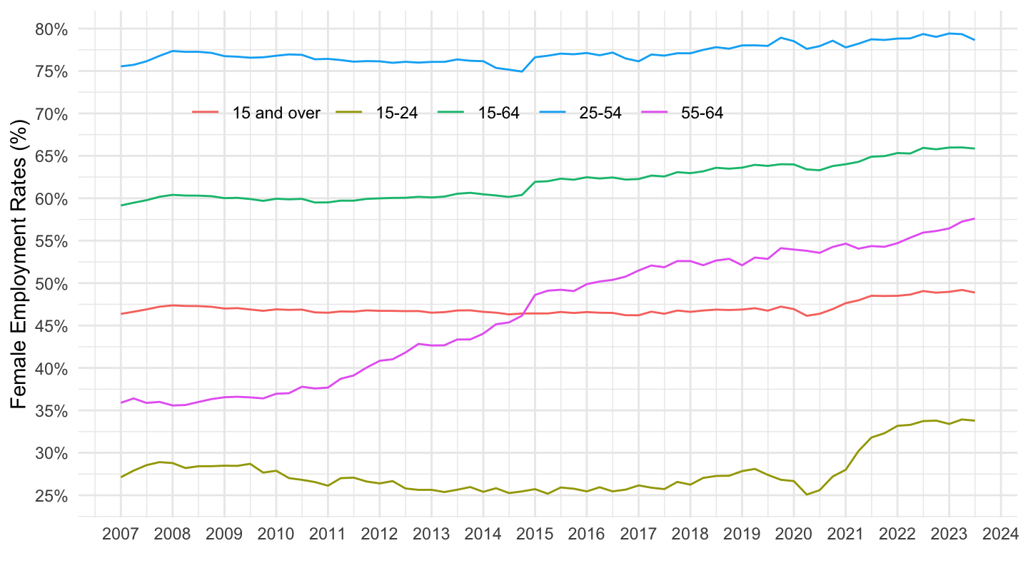

Females, Males

France

Code

MEI |>
  filter(LOCATION %in% c("FRA"),
         SUBJECT %in% c("LREM24FE", "LREM55FE", "LREM25FE", "LREM64FE", "LREMTTFE",
                        "LREM24MA", "LREM55MA", "LREM25MA", "LREM64MA", "LREMTTMA"),
         FREQUENCY == "Q",
         MEASURE == "STSA") |>
  quarter_to_date() |>
  left_join(MEI_var$LOCATION, by = "LOCATION") |>
  left_join(MEI_var$SUBJECT, by = "SUBJECT") |>
  mutate(Gender = ifelse(grepl("Males", Subject), "Males", "Females")) |>
  mutate(obsValue = obsValue / 100,
         Subject = gsub("Labour Force Survey - quarterly rates > Employment rate > Aged ", "", Subject),
         Subject = gsub(" > Females", "", Subject),
         Subject = gsub(" > Males", "", Subject)) |>
  filter(date >= as.Date("2007-01-01")) |>
  ggplot() + geom_line(aes(x = date, y = obsValue, color = Subject, linetype = Gender)) + 
  scale_y_continuous(breaks = 0.01*seq(-10, 100, 5),
                     labels = percent_format(accuracy = 1)) +
  theme_minimal() + xlab("") + ylab("Female Employment Rates (%)") +
  scale_x_date(breaks = seq(1960, 2100, 1) |> paste0("-01-01") |> as.Date(),
               labels = date_format("%Y")) +
  theme(legend.position = c(0.4, 0.75),
        legend.title = element_blank(),
        legend.direction = "horizontal")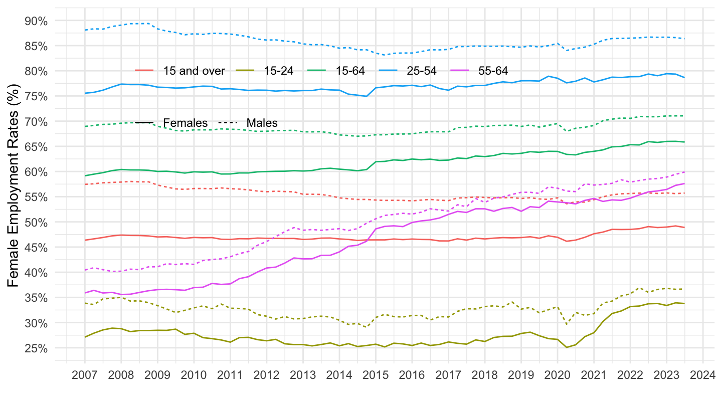

Germany

Code

MEI |>
  filter(LOCATION %in% c("DEU"),
         SUBJECT %in% c("LREM24FE", "LREM55FE", "LREM25FE", "LREM64FE", "LREMTTFE",
                        "LREM24MA", "LREM55MA", "LREM25MA", "LREM64MA", "LREMTTMA"),
         FREQUENCY == "Q",
         MEASURE == "STSA") |>
  quarter_to_date() |>
  left_join(MEI_var$LOCATION, by = "LOCATION") |>
  left_join(MEI_var$SUBJECT, by = "SUBJECT") |>
  mutate(Gender = ifelse(grepl("Males", Subject), "Males", "Females")) |>
  mutate(obsValue = obsValue / 100,
         Subject = gsub("Labour Force Survey - quarterly rates > Employment rate > Aged ", "", Subject),
         Subject = gsub(" > Females", "", Subject),
         Subject = gsub(" > Males", "", Subject)) |>
  filter(date >= as.Date("2007-01-01")) |>
  ggplot() + geom_line(aes(x = date, y = obsValue, color = Subject, linetype = Gender)) + 
  scale_y_continuous(breaks = 0.01*seq(-10, 100, 5),
                     labels = percent_format(accuracy = 1)) +
  theme_minimal() + xlab("") + ylab("Male, Female Employment Rates in Germany (%)") +
  scale_x_date(breaks = seq(1960, 2100, 1) |> paste0("-01-01") |> as.Date(),
               labels = date_format("%Y")) +
  theme(legend.position = c(0.4, 0.75),
        legend.title = element_blank(),
        legend.direction = "horizontal")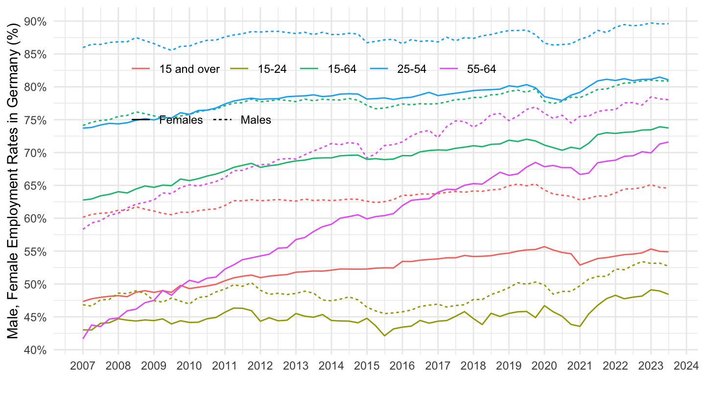

LREM24TT - 15-24

Code

MEI |>
  filter(LOCATION %in% c("FRA", "DEU", "JPN", "USA", "ITA", "ESP", "CHE"),
         SUBJECT == "LREM24TT",
         FREQUENCY == "Q",
         MEASURE == "STSA") |>
  quarter_to_date() |>
  left_join(MEI_var$LOCATION, by = "LOCATION") |>
  left_join(MEI_var$SUBJECT, by = "SUBJECT") |>
  add_flag_color("Location") |>
  mutate(obsValue = obsValue / 100) |>
  filter(date >= as.Date("2007-01-01")) |>
  ggplot() + geom_line(aes(x = date, y = obsValue, color = color)) + 
  scale_color_identity() + add_7flags +
  scale_y_continuous(breaks = 0.01*seq(-10, 100, 2),
                     labels = percent_format(accuracy = 1)) +
  theme_minimal() + xlab("") + ylab("Employment Rates 15-24 (%)") +
  scale_x_date(breaks = seq(1960, 2100, 1) |> paste0("-01-01") |> as.Date(),
               labels = date_format("%Y")) +
  theme(legend.position = "none")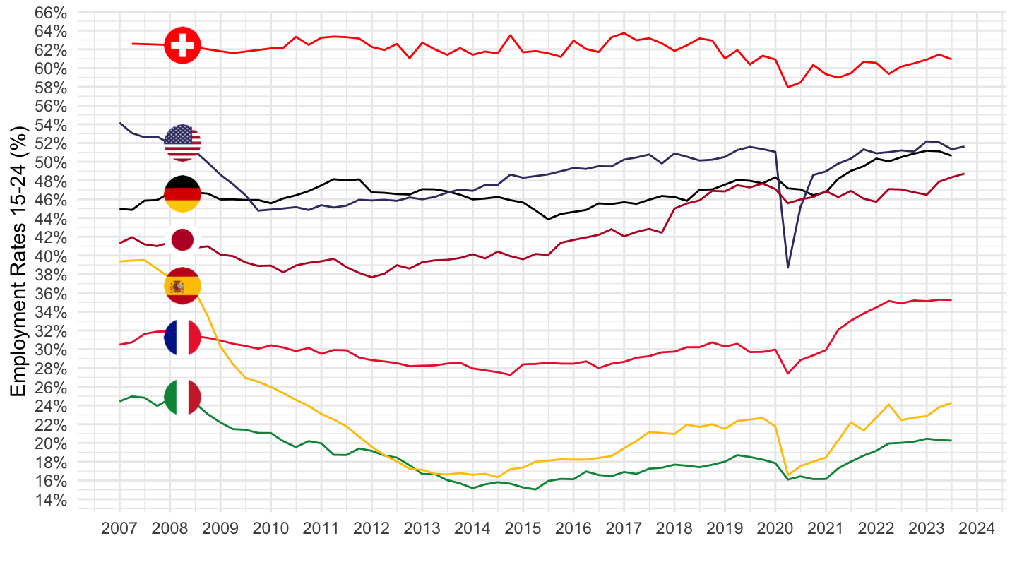

LREM55TT - 55-64

2000-

Code

MEI |>
  filter(LOCATION %in% c("FRA", "DEU", "JPN", "USA", "ITA", "ESP", "CHE"),
         SUBJECT == "LREM55TT",
         FREQUENCY == "Q",
         MEASURE == "STSA") |>
  quarter_to_date() |>
  left_join(MEI_var$LOCATION, by = "LOCATION") |>
  left_join(MEI_var$SUBJECT, by = "SUBJECT") |>
  add_flag_color("Location") |>
  mutate(obsValue = obsValue / 100) |>
  #filter(date >= as.Date("2000-01-01")) %>%
  ggplot() + geom_line(aes(x = date, y = obsValue, color = color)) + 
  scale_color_identity() + add_7flags +
  scale_y_continuous(breaks = 0.01*seq(-10, 100, 2),
                     labels = percent_format(accuracy = 1)) +
  theme_minimal() + xlab("") + ylab("Employment Rates 55-64 (%)") +
  scale_x_date(breaks = seq(1960, 2100, 5) |> paste0("-01-01") |> as.Date(),
               labels = date_format("%Y")) +
  theme(legend.position = "none")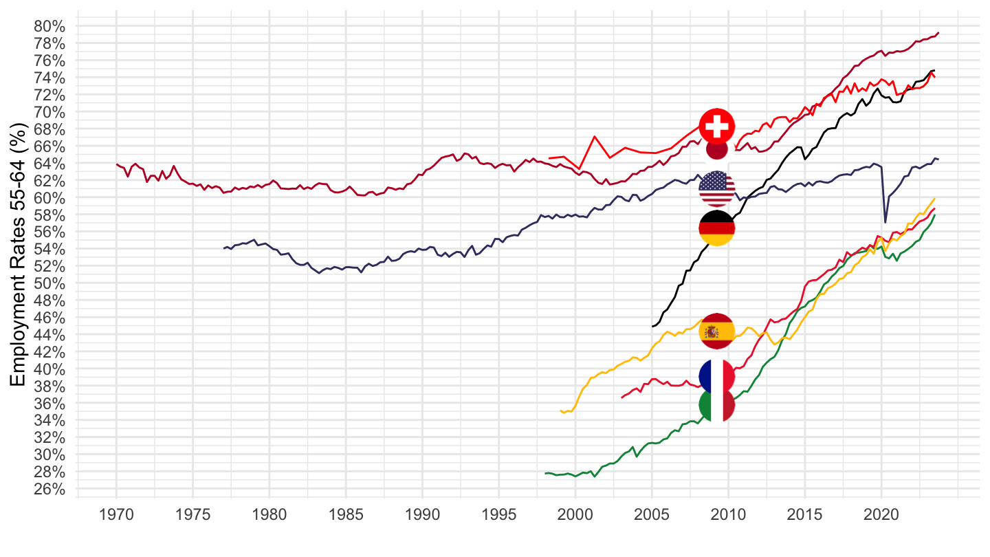

2007-

Code

MEI |>
  filter(LOCATION %in% c("FRA", "DEU", "JPN", "USA", "ITA", "ESP", "CHE"),
         SUBJECT == "LREM55TT",
         FREQUENCY == "Q",
         MEASURE == "STSA") |>
  quarter_to_date() |>
  left_join(MEI_var$LOCATION, by = "LOCATION") |>
  left_join(MEI_var$SUBJECT, by = "SUBJECT") |>
  add_flag_color("Location") |>
  mutate(obsValue = obsValue / 100) |>
  filter(date >= as.Date("2007-01-01")) |>
  ggplot() + geom_line(aes(x = date, y = obsValue, color = color)) + 
  scale_color_identity() + add_7flags +
  scale_y_continuous(breaks = 0.01*seq(-10, 100, 2),
                     labels = percent_format(accuracy = 1)) +
  theme_minimal() + xlab("") + ylab("Employment Rates 55-64 (%)") +
  scale_x_date(breaks = seq(1960, 2100, 1) |> paste0("-01-01") |> as.Date(),
               labels = date_format("%Y")) +
  theme(legend.position = "none")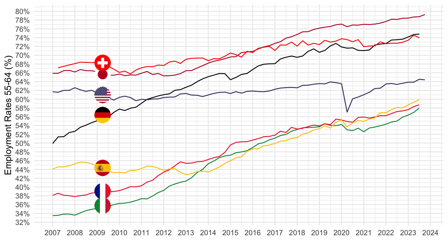

LREM25TT - 25-54

Code

MEI |>
  filter(LOCATION %in% c("FRA", "DEU", "JPN", "USA", "ITA"),
         SUBJECT == "LREM25TT",
         FREQUENCY == "Q",
         MEASURE == "STSA") |>
  quarter_to_date() |>
  left_join(MEI_var$LOCATION, by = "LOCATION") |>
  left_join(MEI_var$SUBJECT, by = "SUBJECT") |>
  add_flag_color("Location") |>
  mutate(obsValue = obsValue / 100) |>
  filter(date >= as.Date("2007-01-01")) |>
  ggplot() + geom_line(aes(x = date, y = obsValue, color = color)) + 
  scale_color_identity() + add_5flags +
  scale_y_continuous(breaks = 0.01*seq(-10, 100, 2),
                     labels = percent_format(accuracy = 1)) +
  theme_minimal() + xlab("") + ylab("Employment Rates 55-64 (%)") +
  scale_x_date(breaks = seq(1960, 2100, 1) |> paste0("-01-01") |> as.Date(),
               labels = date_format("%Y")) +
  theme(legend.position = "none")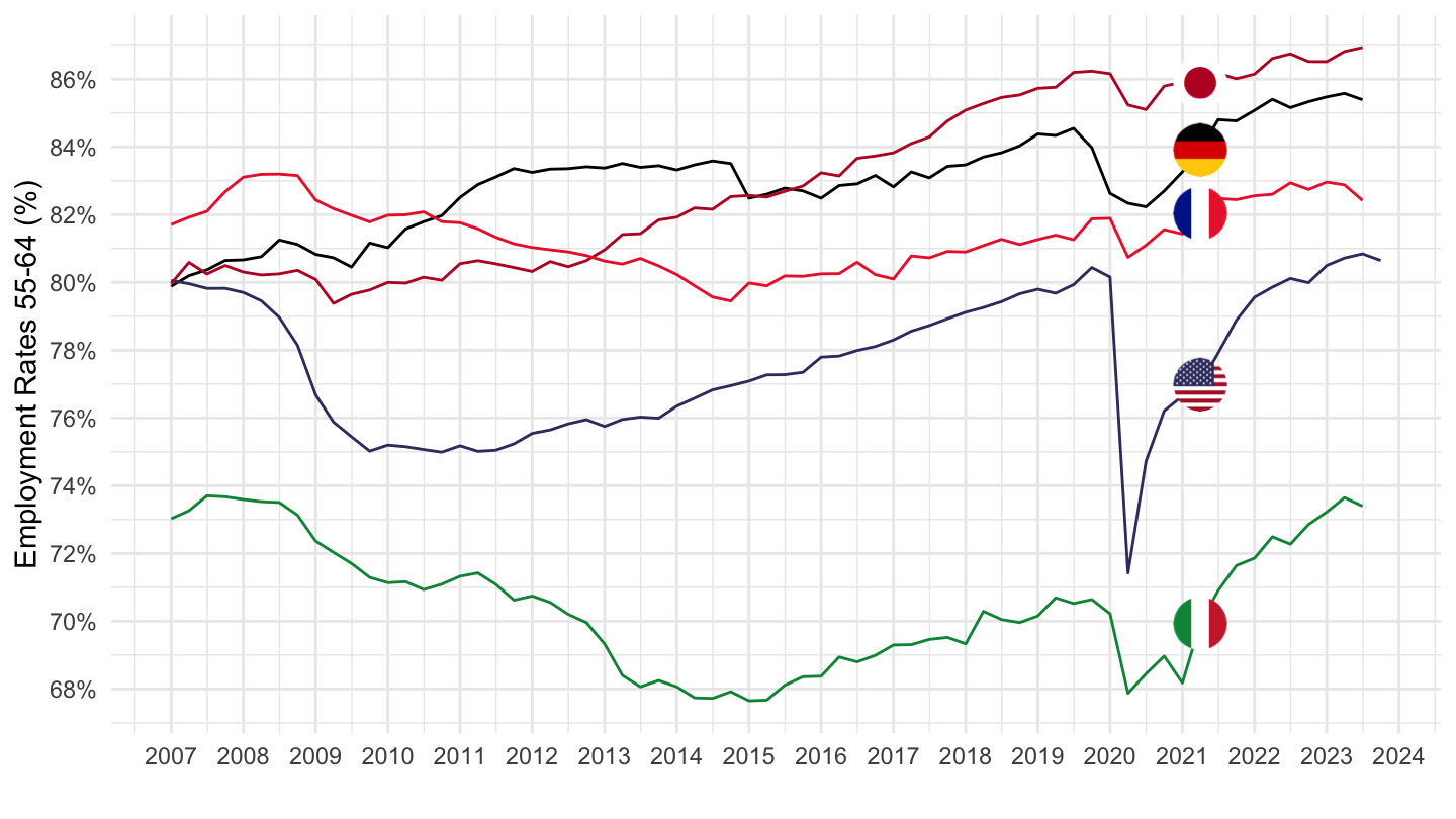

LREM64TT - 15-64

Code

MEI |>
  filter(LOCATION %in% c("FRA", "DEU", "JPN", "USA", "ITA", "ESP", "CHE"),
         SUBJECT == "LREM64TT",
         FREQUENCY == "Q",
         MEASURE == "STSA") |>
  quarter_to_date() |>
  left_join(MEI_var$LOCATION, by = "LOCATION") |>
  left_join(MEI_var$SUBJECT, by = "SUBJECT") |>
  add_flag_color("Location") |>
  mutate(obsValue = obsValue / 100) |>
  filter(date >= as.Date("2007-01-01")) |>
  ggplot() + geom_line(aes(x = date, y = obsValue, color = color)) + 
  scale_color_identity() + add_7flags +
  scale_y_continuous(breaks = 0.01*seq(-10, 100, 2),
                     labels = percent_format(accuracy = 1)) +
  theme_minimal() + xlab("") + ylab("Employment Rates 15-64 (%)") +
  scale_x_date(breaks = seq(1960, 2100, 1) |> paste0("-01-01") |> as.Date(),
               labels = date_format("%Y")) +
  theme(legend.position = "none")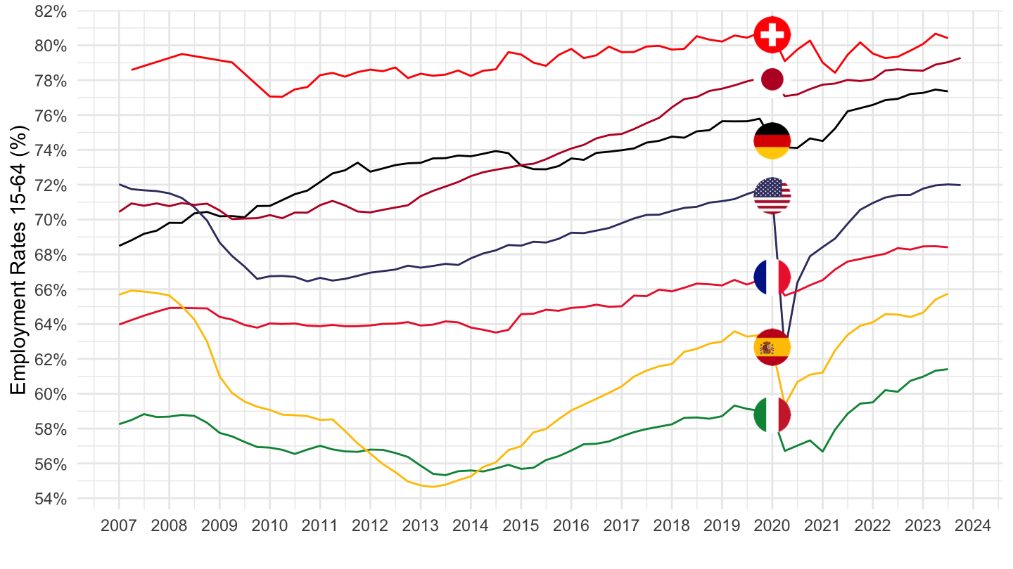

LREMTTTT - 15+

Code

MEI |>
  filter(LOCATION %in% c("FRA", "DEU", "JPN", "USA", "ITA"),
         SUBJECT == "LREMTTTT",
         FREQUENCY == "Q",
         MEASURE == "STSA") |>
  quarter_to_date() |>
  left_join(MEI_var$LOCATION, by = "LOCATION") |>
  left_join(MEI_var$SUBJECT, by = "SUBJECT") |>
  add_flag_color("Location") |>
  mutate(obsValue = obsValue / 100) |>
  filter(date >= as.Date("2007-01-01")) |>
  ggplot() + geom_line(aes(x = date, y = obsValue, color = color)) + 
  scale_color_identity() + add_5flags +
  scale_y_continuous(breaks = 0.01*seq(-10, 100, 2),
                     labels = percent_format(accuracy = 1)) +
  theme_minimal() + xlab("") + ylab("Employment Rates 15+ (%)") +
  scale_x_date(breaks = seq(1960, 2100, 1) |> paste0("-01-01") |> as.Date(),
               labels = date_format("%Y")) +
  theme(legend.position = "none")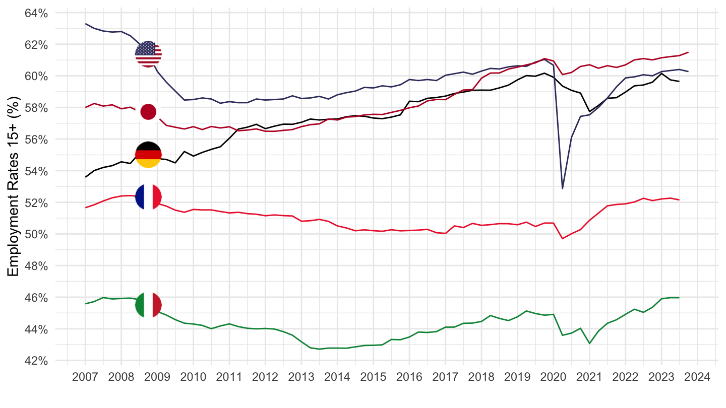

Inflation - CPHPTT01

Table - Countries

Code

MEI |>
  filter(SUBJECT == "CPALTT01",
         FREQUENCY == "M",
         MEASURE == "GY") |>
  left_join(MEI_var$LOCATION, by = "LOCATION") |>
  group_by(LOCATION, Location) |>
  summarise(Nobs = n()) |>
  print_table_conditional()

Table - Countries - EA

Code

MEI |>
  filter(SUBJECT == "CPALTT01",
         FREQUENCY == "M",
         MEASURE == "GY",
         LOCATION %in% c("EA19", "EA20", "EU27_2020", "EU28")) |>
  month_to_date() |>
  left_join(MEI_var$LOCATION, by = "LOCATION") |>
  #filter(date >= as.Date("2019-01-01")) %>%
  ggplot() + geom_line(aes(x = date, y = obsValue, color = Location)) + 
  theme_minimal() + xlab("") + ylab("Consumer Price Index, All items") +
  scale_x_date(breaks = seq(1960, 2100, 1) |> paste0("-01-01") |> as.Date(),
               labels = date_format("%Y")) +
  scale_y_continuous(breaks = 0.01*seq(-10, 200, 1),
                     labels = percent_format(accuracy = 1)) +
  theme(legend.position = c(0.2, 0.80),
        legend.title = element_blank())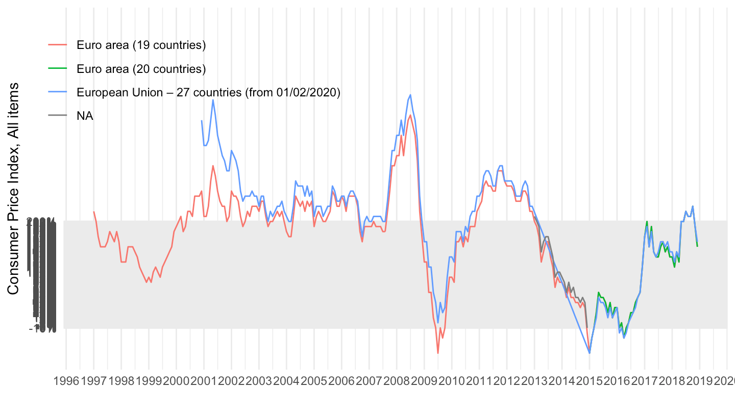

All items

(ref:CPALTT01) Consumer Price Index, All items

Code

MEI |>
  filter(LOCATION %in% c("FRA", "USA", "DEU", "JPN", "EA19"),
         SUBJECT == "CPALTT01",
         FREQUENCY == "M",
         MEASURE == "GY") |>
  month_to_date() |>
  left_join(MEI_var$LOCATION, by = "LOCATION") |>
  add_flag_color("Location") |>
  filter(date >= as.Date("2019-01-01")) |>
  group_by(LOCATION) |>
  mutate(obsValue = obsValue/100) |>
  ggplot() + geom_line(aes(x = date, y = obsValue, color = color)) + 
  scale_color_identity() + add_4flags +
  theme_minimal() + xlab("") + ylab("Consumer Price Index, All items") +
  scale_x_date(breaks = seq(1960, 2100, 1) |> paste0("-01-01") |> as.Date(),
               labels = date_format("%Y")) +
  scale_y_continuous(breaks = 0.01*seq(-10, 200, 1),
                     labels = percent_format(accuracy = 1)) +
  theme(legend.position = c(0.2, 0.80),
        legend.title = element_blank())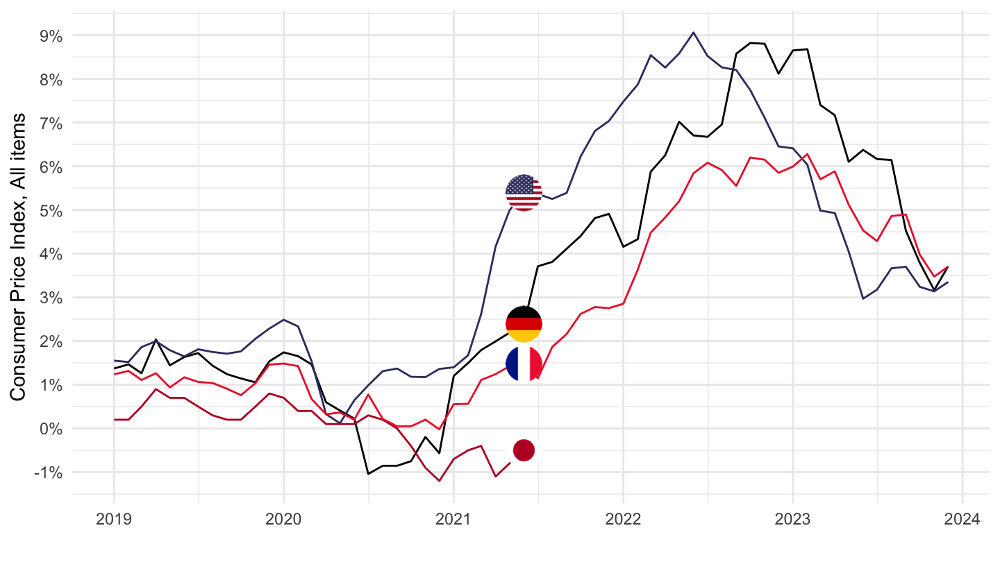

OECD descriptor ID: CPHPTT01 OECD unit ID: GY OECD country ID: EA17

Share Prices - SPASTT01

Nobs

Code

MEI |>
  filter(SUBJECT == "SPASTT01",
         MEASURE == "IXOB",
         FREQUENCY == "M") |>
  left_join(MEI_var$LOCATION, by = c("LOCATION")) |>
  group_by(LOCATION, Location) |>
  summarise(Nobs = n(),
            start = first(obsTime),
            end = last(obsTime)) |>
  arrange(-Nobs) |>
  mutate(Flag = gsub(" ", "-", str_to_lower(gsub(" ", "-", Location))),
         Flag = paste0('<img src="../../icon/flag/vsmall/', Flag, '.png" alt="Flag">')) |>
  select(Flag, everything()) %>%
  {if (is_html_output()) datatable(., filter = 'top', rownames = F, escape = F) else .}

France, United States, Japan

All

Code

MEI |>
  filter(LOCATION %in% c("FRA", "USA", "JPN"),
         SUBJECT == "SPASTT01",
         MEASURE == "IXOB",
         FREQUENCY == "M") |>
  month_to_date() |>
  left_join(MEI_var$LOCATION, by = "LOCATION") |>
  add_flag_color("Location") |>
  ggplot() + geom_line(aes(x = date, y = obsValue, color = color)) + 
  scale_color_identity() + add_3flags + theme_minimal() + xlab("") + ylab("Share Prices") +
  scale_x_date(breaks = seq(1960, 2100, 5) |> paste0("-01-01") |> as.Date(),
               labels = date_format("%Y")) +
  scale_y_log10(breaks = c(1, 2, 5, seq(10, 50, 10), 100, 150, 200, 500, 1000))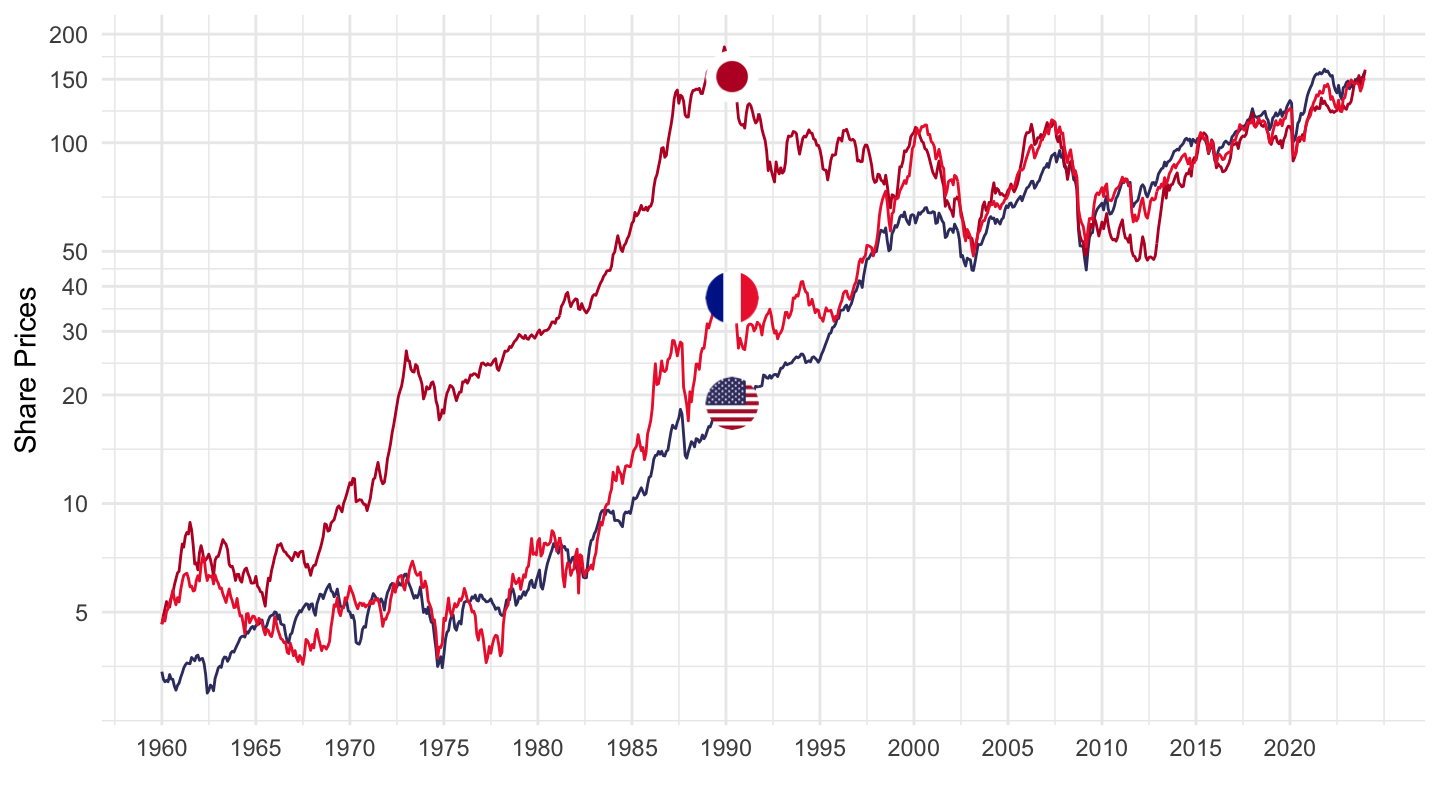

1990-

Code

MEI |>
  filter(LOCATION %in% c("FRA", "USA", "JPN"),
         SUBJECT == "SPASTT01",
         MEASURE == "IXOB",
         FREQUENCY == "M") |>
  month_to_date() |>
  filter(date >= as.Date("1990-01-01")) |>
  left_join(MEI_var$LOCATION, by = "LOCATION") |>
  add_flag_color("Location") |>
  ggplot() + geom_line(aes(x = date, y = obsValue, color = color)) + 
  scale_color_identity() + add_3flags + theme_minimal() + xlab("") + ylab("Share Prices") +
  scale_x_date(breaks = seq(1960, 2100, 5) |> paste0("-01-01") |> as.Date(),
               labels = date_format("%Y")) +
  scale_y_log10(breaks = c(1, 2, 5, seq(10, 50, 10), 100, 150, 200, 500, 1000))

1990-, Base = 100

Code

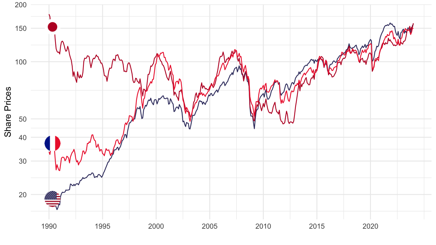
MEI |>
  filter(LOCATION %in% c("FRA", "USA", "JPN"),
         SUBJECT == "SPASTT01",
         MEASURE == "IXOB",
         FREQUENCY == "M") |>
  month_to_date() |>
  filter(date >= as.Date("1990-01-01")) |>
  left_join(MEI_var$LOCATION, by = "LOCATION") |>
  add_flag_color("Location") |>
  group_by(LOCATION) |>
  mutate(obsValue = obsValue/obsValue[1]) |>
  ggplot() + geom_line(aes(x = date, y = obsValue, color = color)) + 
  scale_color_identity() + add_3flags + theme_minimal() + xlab("") + ylab("Share Prices") +
  scale_x_date(breaks = seq(1960, 2100, 5) |> paste0("-01-01") |> as.Date(),
               labels = date_format("%Y")) +
  scale_y_log10(breaks = c(1, 2, 5, seq(10, 50, 10), 100, 150, 200, 500, 1000))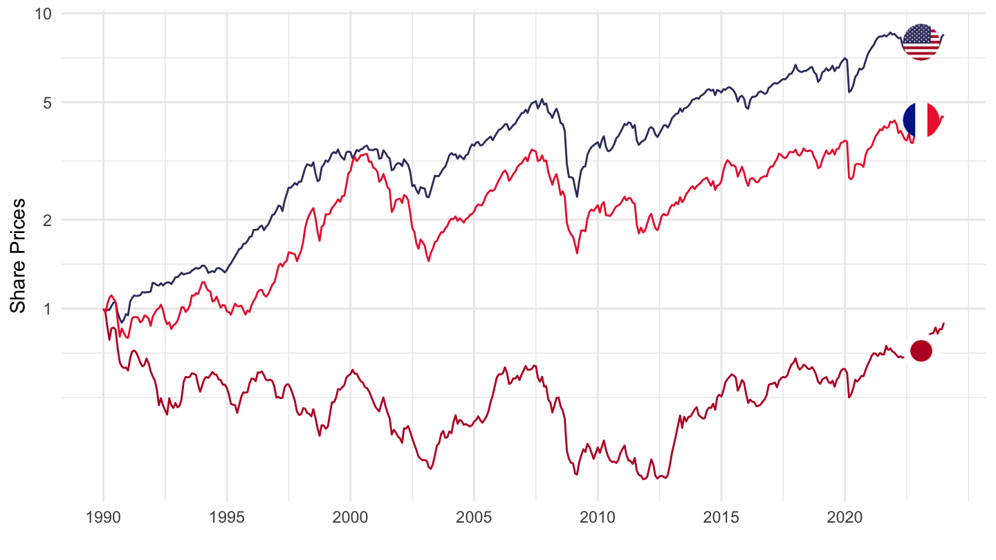

Australia, Austria, Canada

Code

MEI |>
  filter(LOCATION %in% c("AUS", "AUT", "CAN"),
         SUBJECT == "SPASTT01",
         MEASURE == "IXOB",
         FREQUENCY == "M") |>
  month_to_date() |>
  left_join(MEI_var$LOCATION, by = "LOCATION") |>
  add_flag_color("Location") |>
  group_by(LOCATION) |>
  mutate(obsValue = obsValue/obsValue[1]) |>
  ggplot() + geom_line(aes(x = date, y = obsValue, color = color)) + 
  scale_color_identity() + add_3flags + theme_minimal() + xlab("") + ylab("Share Prices") +
  scale_x_date(breaks = seq(1960, 2100, 5) |> paste0("-01-01") |> as.Date(),
               labels = date_format("%Y")) +
  scale_y_log10(breaks = c(1, 2, 5, seq(10, 50, 10), 100, 150, 200, 500, 1000))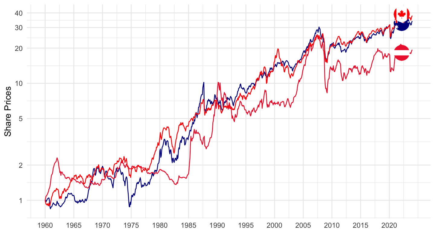

Switzerland, Germany, Finland

Code

MEI |>
  filter(LOCATION %in% c("CHE", "DEU", "FIN"),
         SUBJECT == "SPASTT01",
         MEASURE == "IXOB",
         FREQUENCY == "M") |>
  month_to_date() |>
  left_join(MEI_var$LOCATION, by = "LOCATION") |>
  add_flag_color("Location") |>
  group_by(LOCATION) |>
  mutate(obsValue = obsValue/obsValue[1]) |>
  ggplot() + geom_line(aes(x = date, y = obsValue, color = color)) + 
  scale_color_identity() + add_3flags + theme_minimal() + xlab("") + ylab("Share Prices") +
  scale_x_date(breaks = seq(1960, 2100, 5) |> paste0("-01-01") |> as.Date(),
               labels = date_format("%Y")) +
  scale_y_log10(breaks = c(1, 2, 5, seq(10, 50, 10), 100, 150, 200, 500, 1000))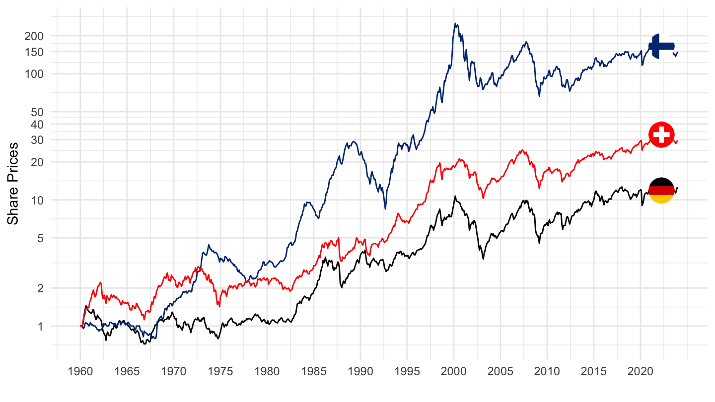

France, United Kingdom, India

Code

MEI |>
  filter(LOCATION %in% c("FRA", "GBR", "IND"),
         SUBJECT == "SPASTT01",
         MEASURE == "IXOB",
         FREQUENCY == "M") |>
  month_to_date() |>
  left_join(MEI_var$LOCATION, by = "LOCATION") |>
  add_flag_color("Location") |>
  group_by(LOCATION) |>
  mutate(obsValue = obsValue/obsValue[1]) |>
  ggplot() + geom_line(aes(x = date, y = obsValue, color = color)) + 
  scale_color_identity() + add_3flags + theme_minimal() + xlab("") + ylab("Share Prices") +
  scale_x_date(breaks = seq(1960, 2100, 5) |> paste0("-01-01") |> as.Date(),
               labels = date_format("%Y")) +
  scale_y_log10(breaks = c(1, 2, 5, seq(10, 50, 10), 100, 150, 200, 500, 1000))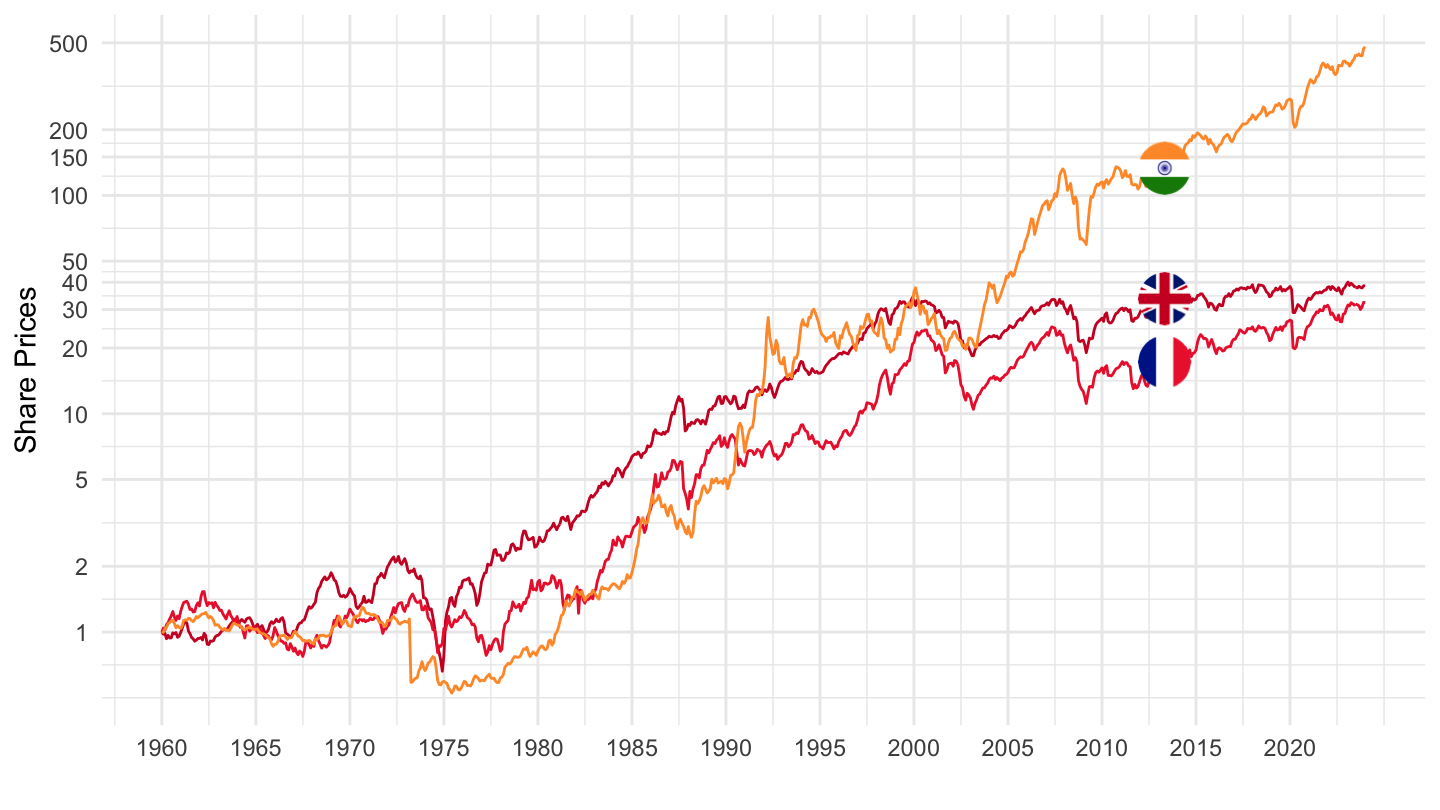

Ireland, Italy, Japan

Code

MEI |>
  filter(LOCATION %in% c("IRL", "ITA", "JPN"),
         SUBJECT == "SPASTT01",
         MEASURE == "IXOB",
         FREQUENCY == "M") |>
  month_to_date() |>
  left_join(MEI_var$LOCATION, by = "LOCATION") |>
  add_flag_color("Location") |>
  group_by(LOCATION) |>
  mutate(obsValue = obsValue/obsValue[1]) |>
  ggplot() + geom_line(aes(x = date, y = obsValue, color = color)) + 
  scale_color_identity() + add_3flags + theme_minimal() + xlab("") + ylab("Share Prices") +
  scale_x_date(breaks = seq(1960, 2100, 5) |> paste0("-01-01") |> as.Date(),
               labels = date_format("%Y")) +
  scale_y_log10(breaks = c(1, 2, 5, seq(10, 50, 10), 100, 150, 200, 500, 1000))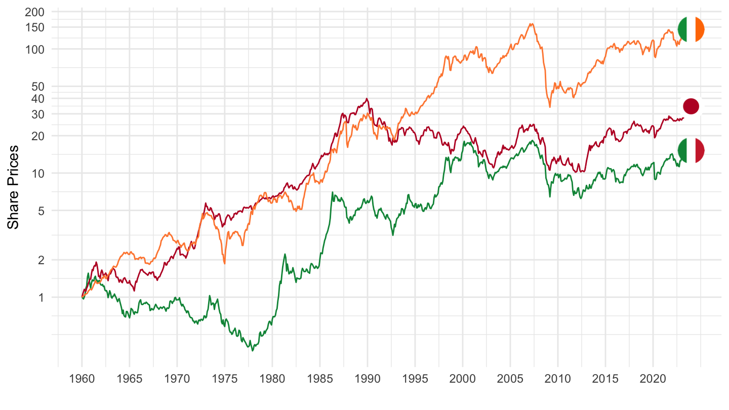

Netherlands, Sweden, United States

Code

MEI |>
  filter(LOCATION %in% c("NLD", "SWE", "USA"),
         SUBJECT == "SPASTT01",
         MEASURE == "IXOB",
         FREQUENCY == "M") |>
  month_to_date() |>
  left_join(MEI_var$LOCATION, by = "LOCATION") |>
  add_flag_color("Location") |>
  group_by(LOCATION) |>
  mutate(obsValue = obsValue/obsValue[1]) |>
  ggplot() + geom_line(aes(x = date, y = obsValue, color = color)) + 
  scale_color_identity() + add_3flags + theme_minimal() + xlab("") + ylab("Share Prices") +
  scale_x_date(breaks = seq(1960, 2100, 5) |> paste0("-01-01") |> as.Date(),
               labels = date_format("%Y")) +
  scale_y_log10(breaks = c(1, 2, 5, seq(10, 50, 10), 100, 150, 200, 500, 1000))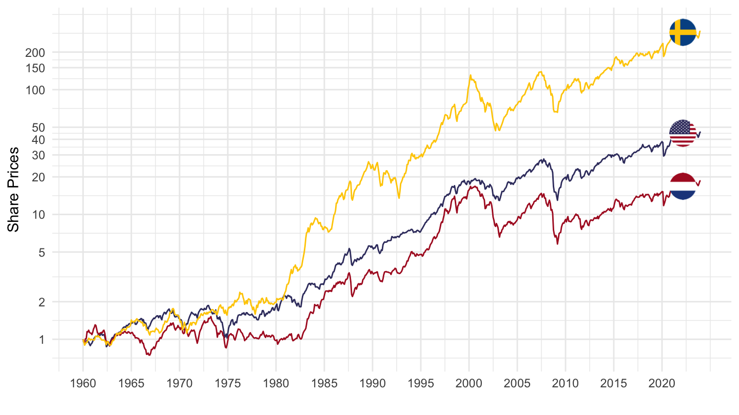

South Africa, New Zealand, Mexico

Code

MEI |>
  filter(LOCATION %in% c("ZAF", "NZL", "MEX"),
         SUBJECT == "SPASTT01",
         MEASURE == "IXOB",
         FREQUENCY == "M") |>
  month_to_date() |>
  left_join(MEI_var$LOCATION, by = "LOCATION") |>
  add_flag_color("Location") |>
  group_by(LOCATION) |>
  mutate(obsValue = obsValue/obsValue[1]) |>
  ggplot() + geom_line(aes(x = date, y = obsValue, color = color)) + 
  scale_color_identity() + add_3flags + theme_minimal() + xlab("") + ylab("Share Prices") +
  scale_x_date(breaks = seq(1960, 2100, 5) |> paste0("-01-01") |> as.Date(),
               labels = date_format("%Y")) +
  scale_y_log10(breaks = c(1, 2, 5, seq(10, 50, 10), 100, 150, 200, 500, 1000))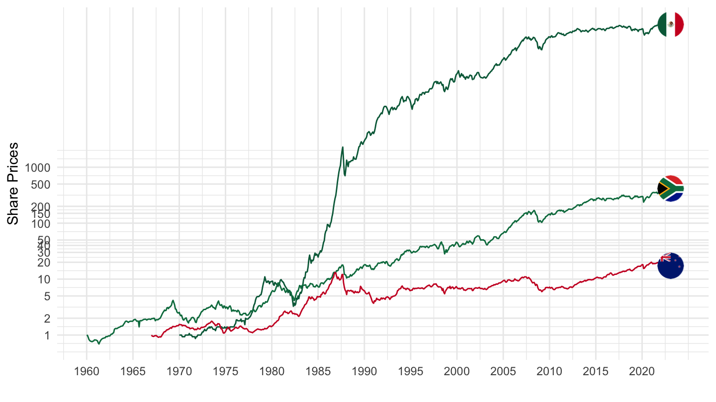

Netherlands, Sweden, United States

Code

MEI |>
  filter(LOCATION %in% c("BRA", "ISR", "KOR"),
         SUBJECT == "SPASTT01",
         MEASURE == "IXOB",
         FREQUENCY == "M") |>
  month_to_date() |>
  left_join(MEI_var$LOCATION, by = "LOCATION") |>
  add_flag_color("Location") |>
  group_by(LOCATION) |>
  mutate(obsValue = obsValue/obsValue[1]) |>
  ggplot() + geom_line(aes(x = date, y = obsValue, color = color)) + 
  scale_color_identity() + add_3flags + theme_minimal() + xlab("") + ylab("Share Prices") +
  scale_x_date(breaks = seq(1960, 2100, 5) |> paste0("-01-01") |> as.Date(),
               labels = date_format("%Y")) +
  scale_y_log10(breaks = c(1, 2, 5, seq(10, 50, 10), 100, 150, 200, 500, 1000))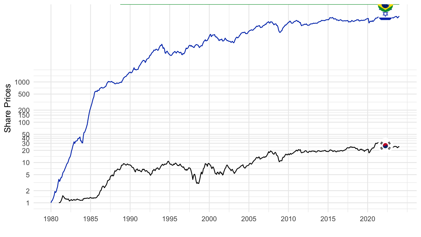

CA Balance

Code

MEI |>
  filter(LOCATION %in% c("FRA", "USA", "DEU", "JPN"),
         SUBJECT == "B6BLTT02",
         FREQUENCY == "Q") |>
  quarter_to_date() |>
  left_join(MEI_var$LOCATION, by = "LOCATION") |>
  add_flag_color("Location") |>
  group_by(LOCATION) |>
  ggplot() + geom_line(aes(x = date, y = obsValue / 100, color = color)) + 
  scale_color_identity() + add_3flags +
  theme_minimal() + xlab("") + ylab("Total CA Balance, % of GDP") +
  scale_x_date(breaks = seq(1960, 2100, 5) |> paste0("-01-01") |> as.Date(),
               labels = date_format("%Y")) +
  scale_y_continuous(breaks = 0.01*seq(-10, 50, 1),
                     labels = percent_format(accuracy = 1)) +
  theme(legend.position = c(0.2, 0.80),
        legend.title = element_blank())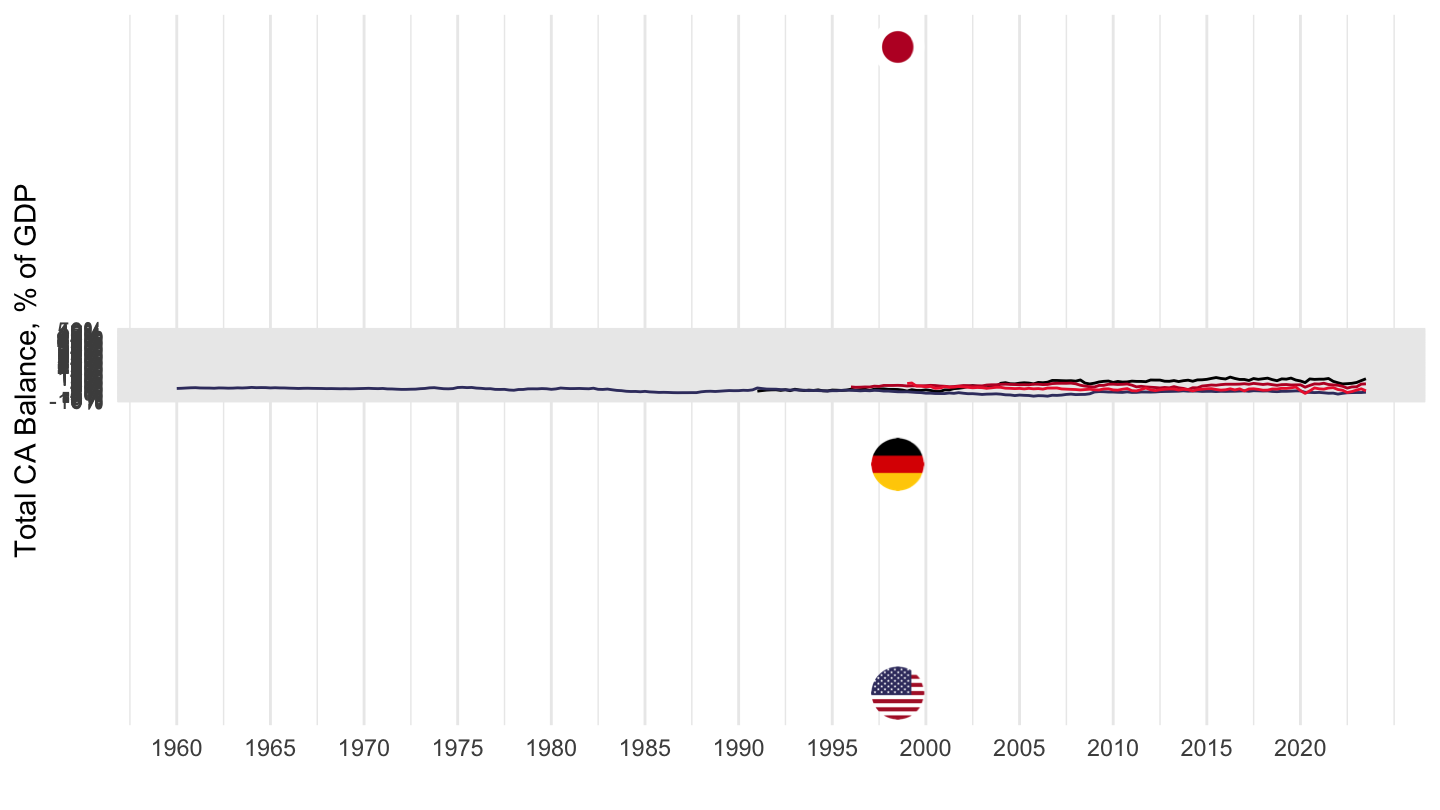

Housing excl imputed rentals for housing

(ref:CPGRHO02) Housing excluding imputed rentals for housing

Code

MEI |>
  filter(LOCATION %in% c("FRA", "USA", "DEU", "JPN"),
         SUBJECT == "CPGRHO02",
         MEASURE == "IXOB",
         FREQUENCY == "Q") |>
  quarter_to_date() |>
  left_join(MEI_var$LOCATION, by = "LOCATION") |>
  add_flag_color("Location") |>
  group_by(LOCATION) |>
  ggplot() + geom_line(aes(x = date, y = obsValue, color = color)) + 
  scale_color_identity() + add_3flags +
  theme_minimal() + xlab("") + ylab("CPI") +
  scale_x_date(breaks = seq(1960, 2100, 5) |> paste0("-01-01") |> as.Date(),
               labels = date_format("%Y")) +
  scale_y_continuous(breaks = seq(-10, 200, 10),
                     labels = dollar_format(accuracy = 1, prefix = "")) +
  theme(legend.position = c(0.2, 0.80),
        legend.title = element_blank())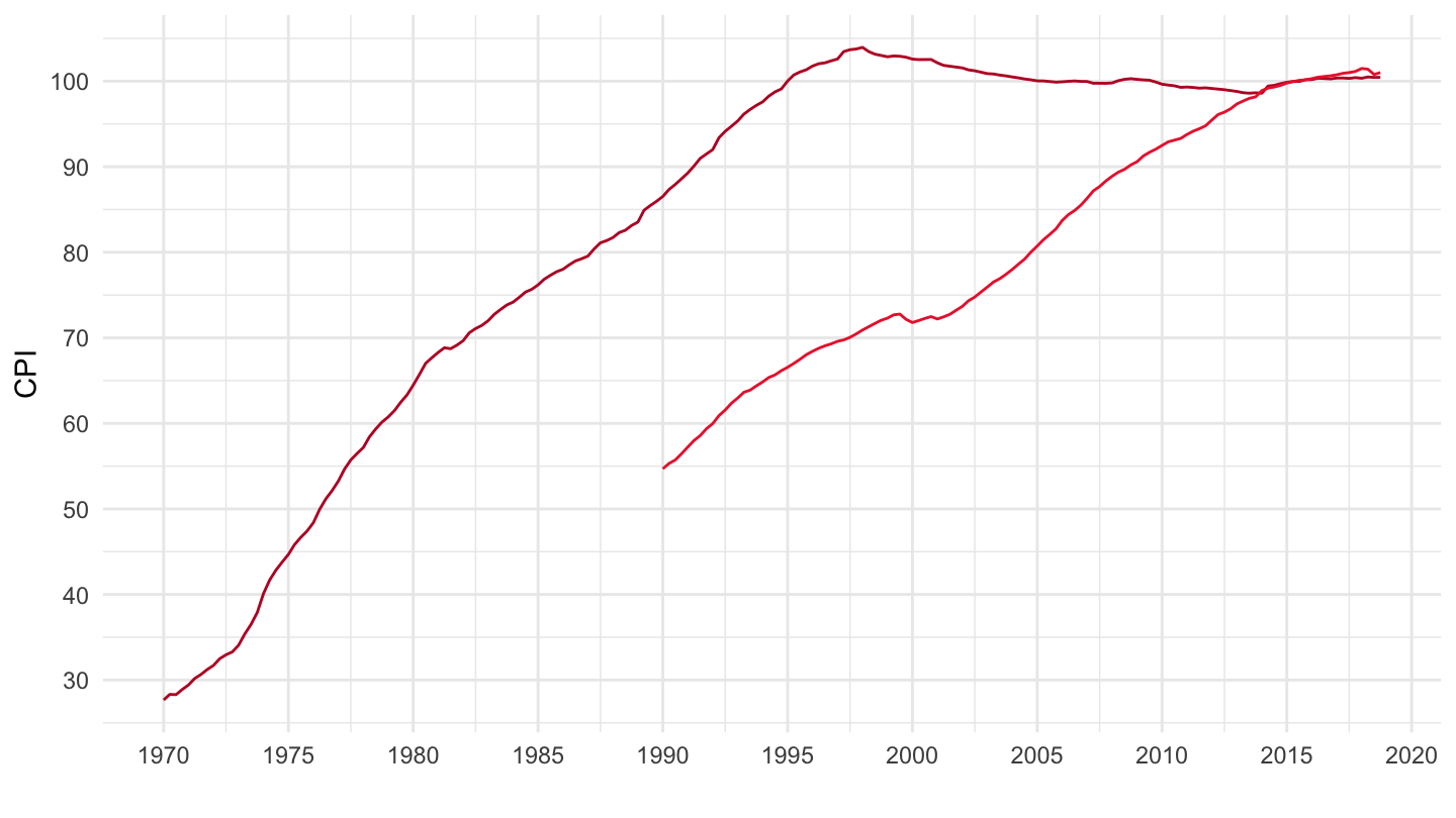

CPI

All items

(ref:CPALTT01) Consumer Price Index, All items

Code

MEI |>
  filter(LOCATION %in% c("FRA", "USA", "DEU", "JPN"),
         SUBJECT == "CPALTT01",
         FREQUENCY == "Q",
         MEASURE == "IXOB") |>
  quarter_to_date() |>
  left_join(MEI_var$LOCATION, by = "LOCATION") |>
  add_flag_color("Location") |>
  group_by(LOCATION) |>
  ggplot() + geom_line(aes(x = date, y = obsValue, color = color)) + 
  scale_color_identity() + add_3flags +
  theme_minimal() + xlab("") + ylab("Consumer Price Index, All items") +
  scale_x_date(breaks = seq(1960, 2100, 5) |> paste0("-01-01") |> as.Date(),
               labels = date_format("%Y")) +
  scale_y_continuous(breaks = seq(-10, 200, 10),
                     labels = dollar_format(accuracy = 1, prefix = "")) +
  theme(legend.position = c(0.2, 0.80),
        legend.title = element_blank())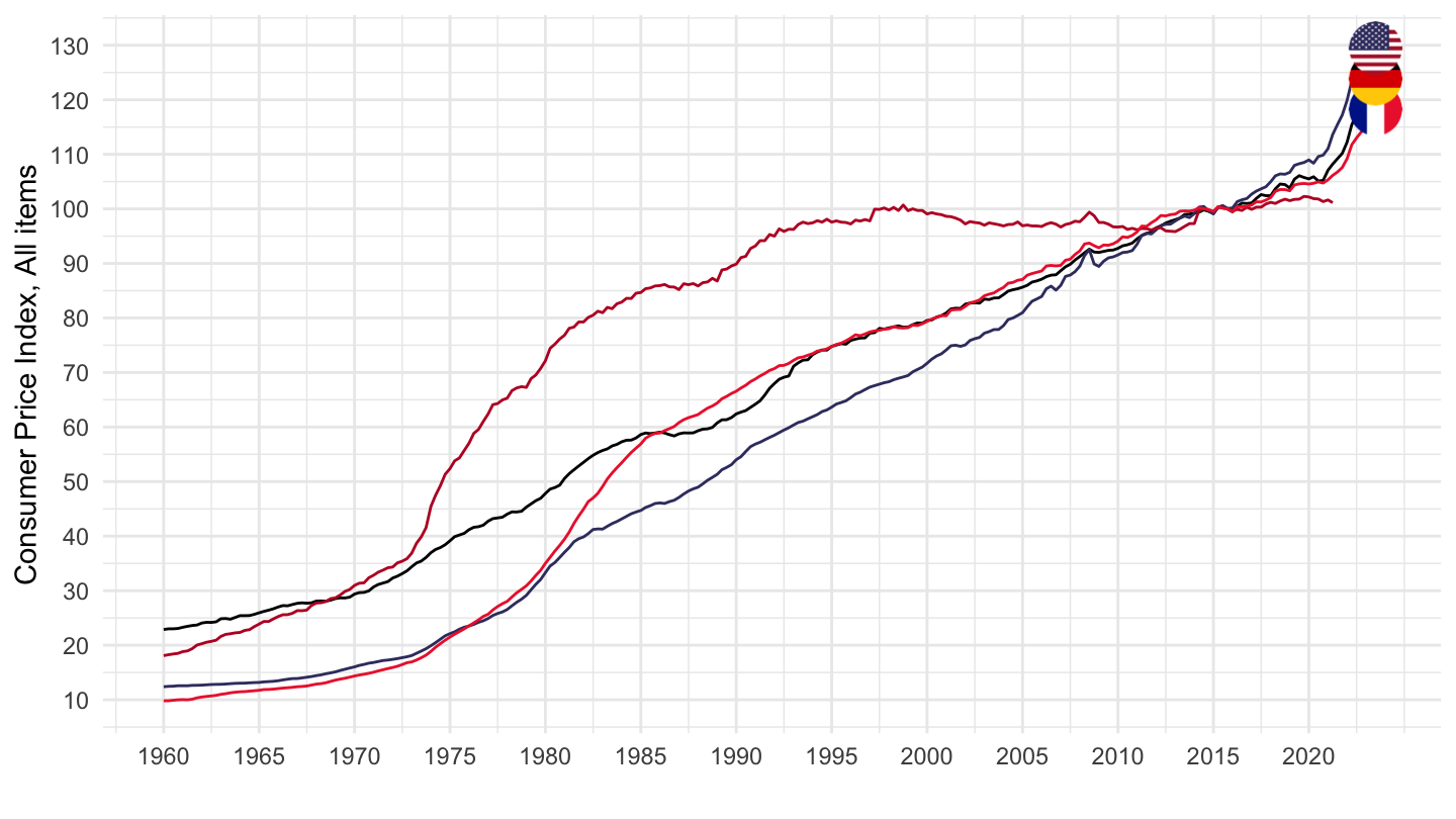

Services less housing

(ref:CPGRLH01) Consumer Price Index, Services less housing

Code

MEI |>
  filter(LOCATION %in% c("FRA", "USA", "DEU", "JPN"),
         SUBJECT == "CPGRLH01",
         FREQUENCY == "Q",
         MEASURE == "IXOB") |>
  quarter_to_date() |>
  left_join(MEI_var$LOCATION, by = "LOCATION") |>
  add_flag_color("Location") |>
  group_by(LOCATION) |>
  ggplot() + geom_line(aes(x = date, y = obsValue, color = color)) + 
  scale_color_identity() + add_3flags +
  theme_minimal() + xlab("") + ylab("Services less housing") +
  scale_x_date(breaks = seq(1960, 2100, 5) |> paste0("-01-01") |> as.Date(),
               labels = date_format("%Y")) +
  scale_y_continuous(breaks = seq(-10, 200, 10),
                     labels = dollar_format(accuracy = 1, prefix = "")) +
  theme(legend.position = c(0.2, 0.80),
        legend.title = element_blank())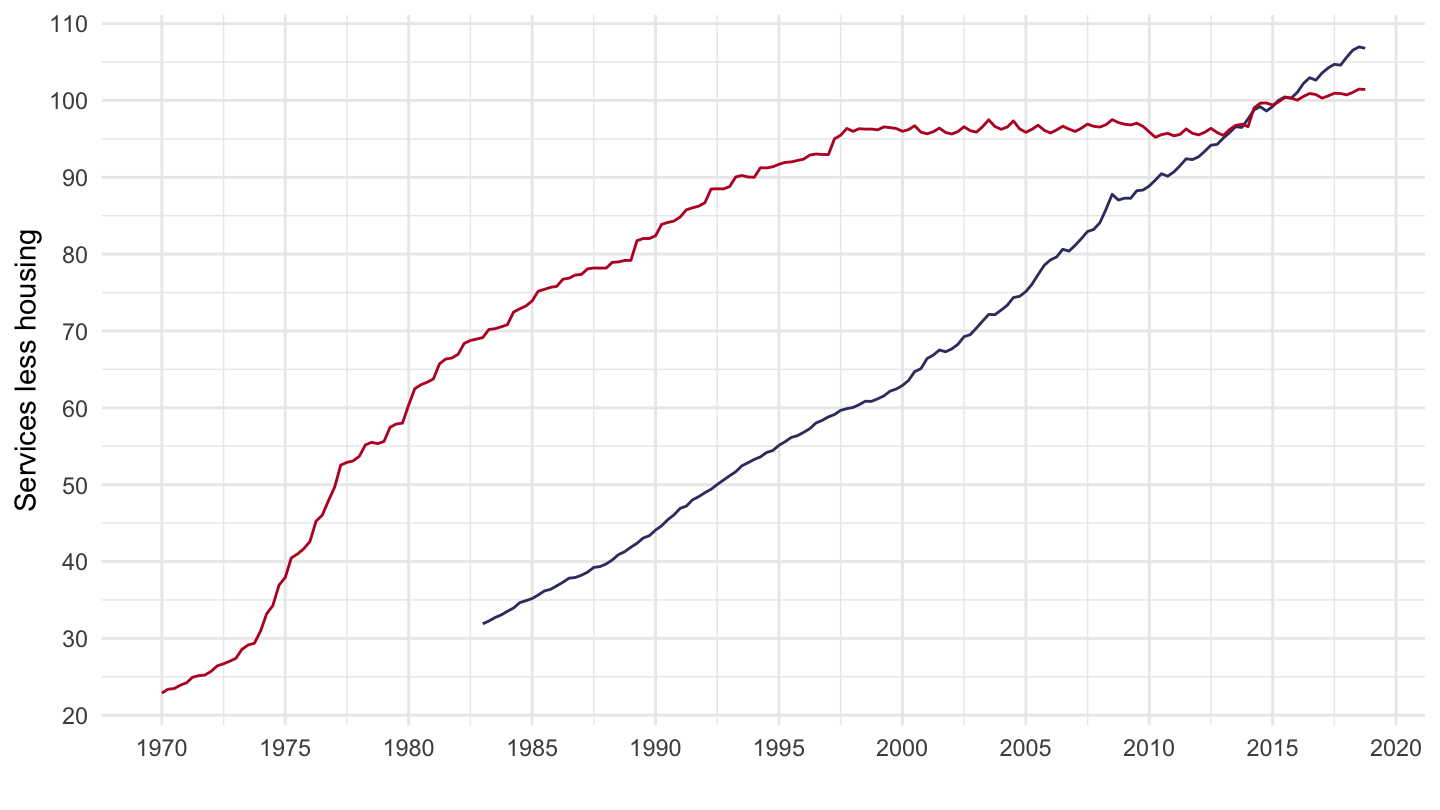

Food and non-Alcoholic beverages

(ref:CP010000) CPI, Food and non-Alcoholic beverages

Code

MEI |>
  filter(LOCATION %in% c("FRA", "USA", "DEU", "JPN"),
         SUBJECT == "CP010000",
         FREQUENCY == "Q",
         MEASURE == "IXOB") |>
  quarter_to_date() |>
  left_join(MEI_var$LOCATION, by = "LOCATION") |>
  add_flag_color("Location") |>
  group_by(LOCATION) |>
  ggplot() + geom_line(aes(x = date, y = obsValue, color = color)) + 
  scale_color_identity() + add_3flags +
  theme_minimal() + xlab("") + ylab("CPI, Food and non-Alcoholic beverages") +
  scale_x_date(breaks = seq(1960, 2100, 5) |> paste0("-01-01") |> as.Date(),
               labels = date_format("%Y")) +
  scale_y_continuous(breaks = seq(-10, 200, 10),
                     labels = dollar_format(accuracy = 1, prefix = "")) +
  theme(legend.position = c(0.2, 0.80),
        legend.title = element_blank())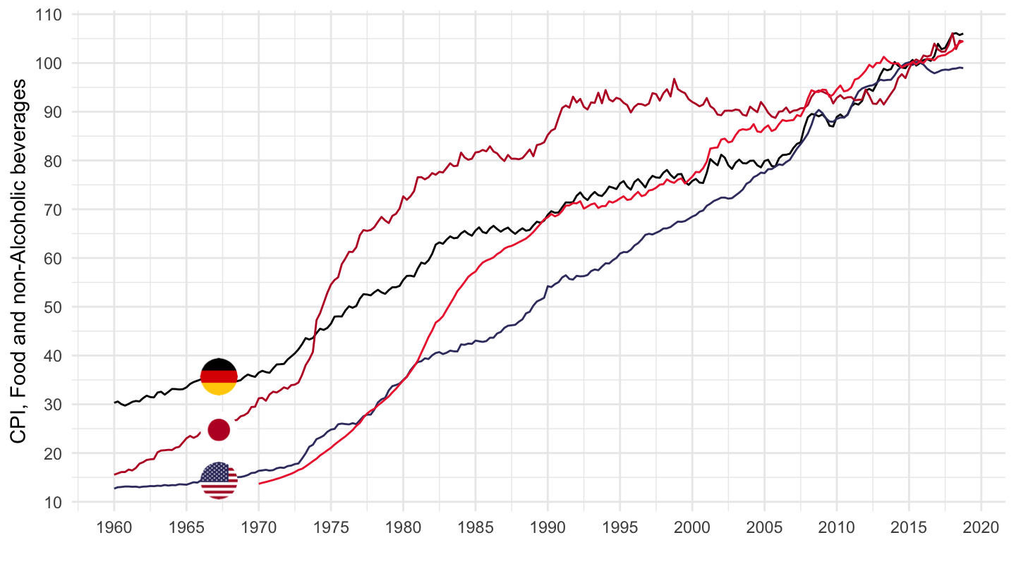

Clothing and Footware

(ref:CP030000) CPI, Clothing and Footware

Code

MEI |>
  filter(LOCATION %in% c("FRA", "USA", "DEU", "JPN"),
         SUBJECT == "CP030000",
         FREQUENCY == "Q",
         MEASURE == "IXOB") |>
  quarter_to_date() |>
  left_join(MEI_var$LOCATION, by = "LOCATION") |>
  add_flag_color("Location") |>
  group_by(LOCATION) |>
  ggplot() + geom_line(aes(x = date, y = obsValue, color = color)) + 
  scale_color_identity() + add_3flags +
  theme_minimal() + xlab("") + ylab("CPI, Clothing and Footware") +
  scale_x_date(breaks = seq(1960, 2100, 5) |> paste0("-01-01") |> as.Date(),
               labels = date_format("%Y")) +
  scale_y_continuous(breaks = seq(-10, 200, 10),
                     labels = dollar_format(accuracy = 1, prefix = "")) +
  theme(legend.position = c(0.2, 0.80),
        legend.title = element_blank())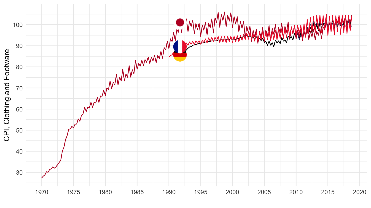

Restaurants and hotels

(ref:CP110000) CPI, Restaurants and hotels

Code

MEI |>
  filter(LOCATION %in% c("FRA", "USA", "DEU", "JPN"),
         SUBJECT == "CP110000",
         FREQUENCY == "Q",
         MEASURE == "IXOB") |>
  quarter_to_date() |>
  left_join(MEI_var$LOCATION, by = "LOCATION") |>
  add_flag_color("Location") |>
  group_by(LOCATION) |>
  ggplot() + geom_line(aes(x = date, y = obsValue, color = color)) + 
  scale_color_identity() + add_3flags +
  theme_minimal() + xlab("") + ylab("CPI,  Restaurants and hotels") +
  scale_x_date(breaks = seq(1960, 2100, 5) |> paste0("-01-01") |> as.Date(),
               labels = date_format("%Y")) +
  scale_y_continuous(breaks = seq(-10, 200, 10),
                     labels = dollar_format(accuracy = 1, prefix = "")) +
  theme(legend.position = c(0.2, 0.80),
        legend.title = element_blank())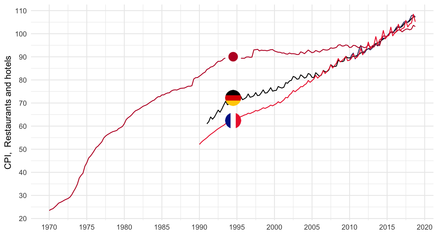

Actual rentals for housing

Code

MEI |>
  filter(LOCATION %in% c("FRA", "USA", "DEU", "JPN"),
         SUBJECT == "CP040100",
         FREQUENCY == "Q",
         MEASURE == "IXOB") |>
  quarter_to_date() |>
  left_join(MEI_var$LOCATION, by = "LOCATION") |>
  add_flag_color("Location") |>
  group_by(LOCATION) |>
  ggplot() + geom_line(aes(x = date, y = obsValue, color = color)) + 
  scale_color_identity() + add_3flags +
  theme_minimal() + xlab("") + ylab("CPI, Actual rentals for housing") +
  scale_x_date(breaks = seq(1960, 2100, 5) |> paste0("-01-01") |> as.Date(),
               labels = date_format("%Y")) +
  scale_y_continuous(breaks = seq(-10, 200, 10),
                     labels = dollar_format(accuracy = 1, prefix = "")) +
  theme(legend.position = c(0.2, 0.80),
        legend.title = element_blank())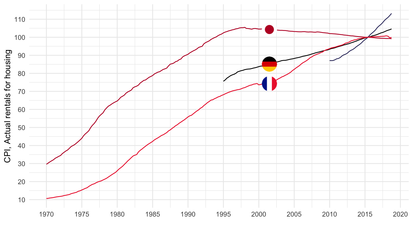

Exchange Rates

Code

MEI |>
  filter(LOCATION %in% c("FRA", "DEU", "ITA"),
         # CCUSMA02: Average of daily rates > National currency:USD
         SUBJECT == "CCUSMA02",
         # ST: Level, rate or national currency
         MEASURE == "ST",
         FREQUENCY == "Q") |>
  quarter_to_date() |>
  left_join(MEI_var$LOCATION, by = "LOCATION") |>
  add_flag_color("Location") |>
  group_by(LOCATION) |>
  ggplot() + geom_line(aes(x = date, y = obsValue, color = color)) + 
  scale_color_identity() + add_3flags +
  theme_minimal() + xlab("") + ylab("Exchange Rate ($1 = ?National Currency)") +
  scale_x_date(breaks = seq(1960, 2100, 5) |> paste0("-01-01") |> as.Date(),
               labels = date_format("%Y")) +
  scale_y_continuous(breaks = seq(0, 10, 0.2),
                     labels = dollar_format(accuracy = 0.1, prefix = "", suffix = "../$")) +
  theme(legend.position = c(0.8, 0.80),
        legend.title = element_blank())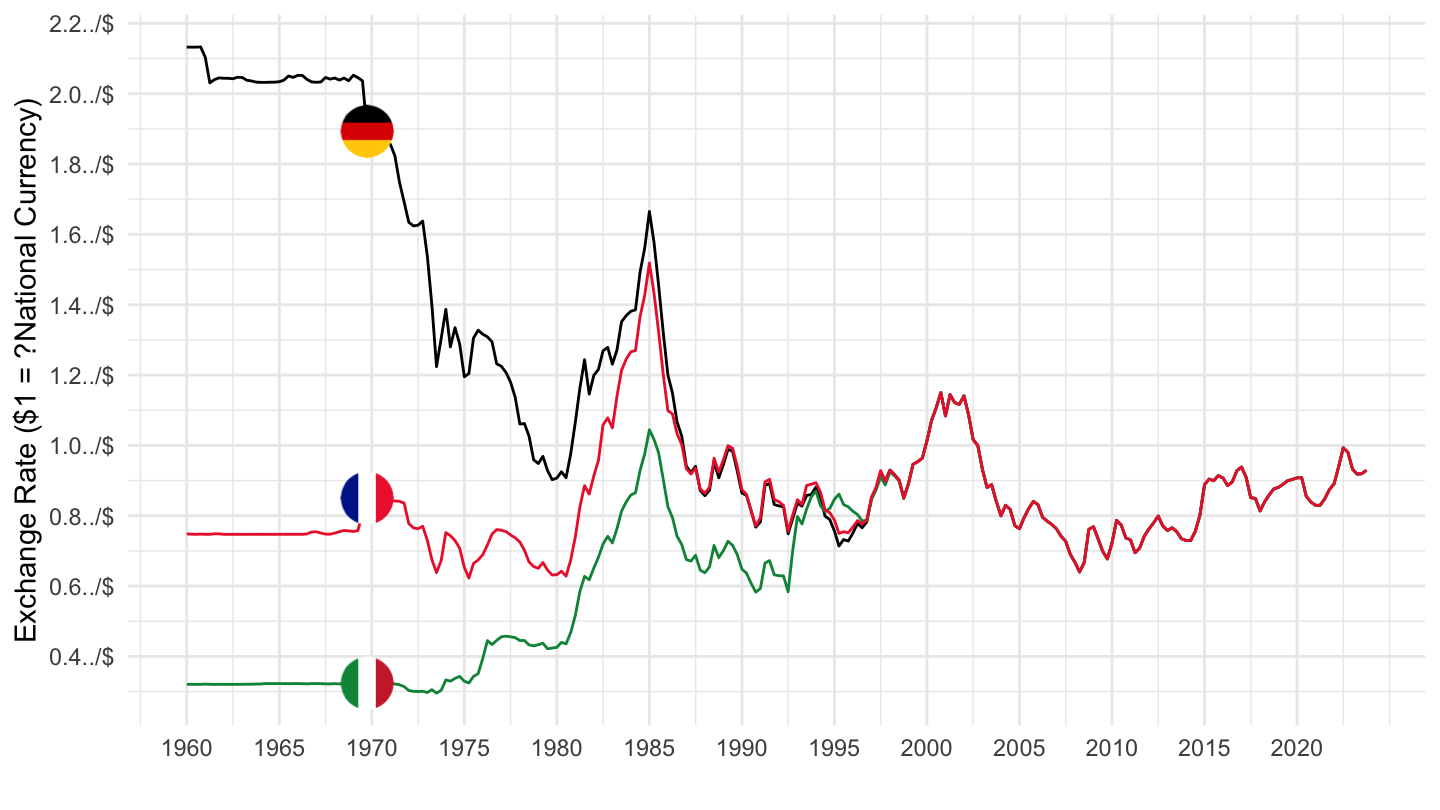

Passenger cars

Example

Code

MEI |>
  filter(LOCATION %in% c("FRA", "DEU", "ITA"),
         # SLRTCR03: Passenger cars
         SUBJECT == "SLRTCR03",
         # ML: Monthly level
         MEASURE == "ML",
         FREQUENCY == "M") |>
  month_to_date() |>
  left_join(MEI_var$LOCATION, by = "LOCATION") |>
  add_flag_color("Location") |>
  group_by(LOCATION) |>
  mutate(obsValue = obsValue/10^3) |>
  ggplot() + geom_line(aes(x = date, y = obsValue, color = color)) + 
  scale_color_identity() + add_3flags +
  theme_minimal() + xlab("") + ylab("") +
  scale_x_date(breaks = seq(1960, 2100, 5) |> paste0("-01-01") |> as.Date(),
               labels = date_format("%Y")) +
  scale_y_continuous(breaks = seq(0, 1000, 50),
                     labels = dollar_format(accuracy = 1, prefix = "", suffix = "K")) +
  theme(legend.position = c(0.2, 0.80),
        legend.title = element_blank())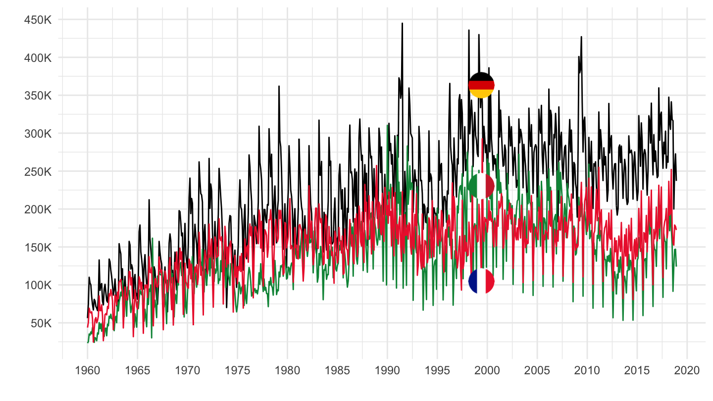

Example

Code

MEI |>
  filter(LOCATION %in% c("FRA", "DEU", "ITA","USA"),
         # SLRTCR03: Passenger cars
         SUBJECT == "SLRTCR03",
         # ML: Monthly level
         MEASURE == "ML",
         FREQUENCY == "A") |>
  year_to_date() |>
  left_join(MEI_var$LOCATION, by = "LOCATION") |>
  add_flag_color("Location") |>
  group_by(LOCATION) |>
  mutate(obsValue = obsValue/10^3) |>
  ggplot() + geom_line(aes(x = date, y = obsValue, color = color)) + 
  scale_color_identity() + add_3flags +
  theme_minimal() + xlab("") + ylab("") +
  scale_x_date(breaks = seq(1960, 2100, 5) |> paste0("-01-01") |> as.Date(),
               labels = date_format("%Y")) +
  scale_y_continuous(breaks = seq(0, 1000, 50),
                     labels = dollar_format(accuracy = 1, prefix = "", suffix = "K")) +
  theme(legend.position = c(0.2, 0.80),
        legend.title = element_blank())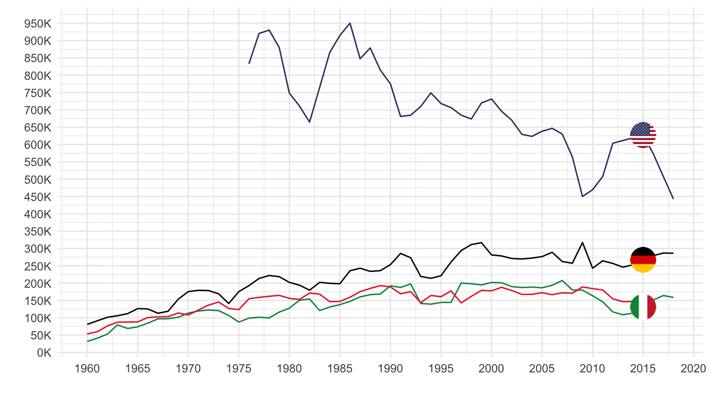

Current Account Balance

Code

MEI |>
  filter(LOCATION %in% c("FRA", "DEU", "ITA"),
         # B6BLTT01: Balance of payments BPM6 > Current account Balance > Total > Total Balance
         SUBJECT == "B6BLTT01",
         # CXCUSA: US Dollars, sum over component sub-periods, s.a
         MEASURE == "CXCUSA",
         FREQUENCY == "Q") |>
  quarter_to_date() |>
  left_join(MEI_var$LOCATION, by = "LOCATION") |>
  add_flag_color("Location") |>
  group_by(LOCATION) |>
  mutate(obsValue = obsValue/10^3) |>
  ggplot() + geom_line(aes(x = date, y = obsValue, color = color)) + 
  scale_color_identity() + add_3flags +
  theme_minimal() +
  theme(legend.title = element_blank(),
        legend.position = c(0.2, 0.8)) +
  scale_x_date(breaks = seq(1950, 2100, 5) |> paste0("-01-01") |> as.Date(),
               labels = date_format("%Y")) +
  scale_y_continuous(breaks = seq(-20000, 400000, 10),
                     labels = dollar_format(accuracy = 1, suffix = " Bn", prefix = "$ ")) + 
  xlab("") + ylab("Current account Balance, Total")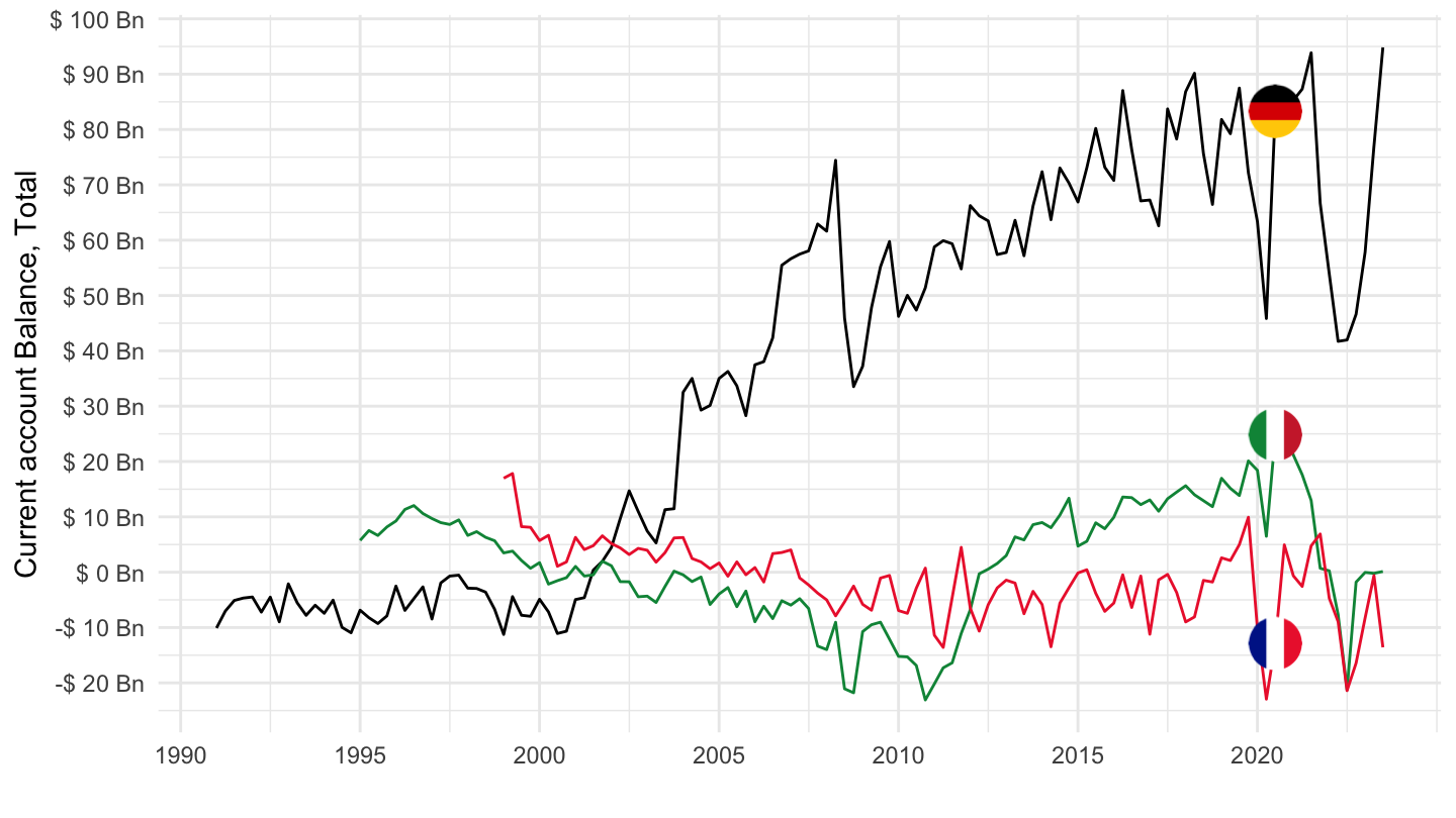

Related Data

Data on interest rates

source	dataset	Title	Updated
oecd	MEI	Main Economic Indicators - MEI	2026-08-02
bdf	FM	Marché financier, taux - FM	2026-08-31
bdf	MIR	Taux d'intérêt - Zone euro - MIR	2026-08-28
bdf	MIR1	Taux d'intérêt - France - MIR1	2026-08-28
bis	CBPOL_D	NA	NA
bis	CBPOL_M	NA	NA
ecb	FM	Financial market data - FM	2026-08-31
ecb	MIR	MFI Interest Rate Statistics - MIR	2026-09-01
eurostat	ei_mfir_m	Interest rates - monthly data - ei_mfir_m	2026-08-14
eurostat	irt_lt_mcby_d	NA	NA
eurostat	irt_st_m	Money market interest rates - monthly data - irt_st_m	2026-08-13
fred	r	Interest Rates - r	2026-09-01
oecd	MEI_FIN	Monthly Monetary and Financial Statistics (MEI) - MEI_FIN	2026-08-02
wdi	FR.INR.DPST	Deposit interest rate (%) - FR.INR.DPST	2026-09-01
wdi	FR.INR.LEND	Lending interest rate (%) - FR.INR.LEND	2026-08-30
wdi	FR.INR.RINR	Real interest rate (%) - FR.INR.RINR	2026-09-01