Household Dashboard

Data - OECD


Info

Data on wages

Code
wages %>%
  arrange(-(dataset == "HH_DASH")) %>%
  mutate(Title = read_lines(paste0("~/Library/Mobile\ Documents/com~apple~CloudDocs/website/data/", source, "/",dataset, ".qmd"), skip = 1, n_max = 1) %>% gsub("title: ", "", .) %>% gsub("\"", "", .)) %>%
  mutate(Download = as.Date(file.info(paste0("~/Library/Mobile\ Documents/com~apple~CloudDocs/website/data/", source, "/", dataset, ".RData"))$mtime),
         Compile = as.Date(file.info(paste0("~/Library/Mobile\ Documents/com~apple~CloudDocs/website/data/", source, "/", dataset, ".html"))$mtime)) %>%
  mutate(Compile = paste0("[", Compile, "](https://fgeerolf.com/data/", source, "/", dataset, '.html)')) %>%
  print_table_conditional_20()
source dataset Title Download Compile
oecd HH_DASH Household Dashboard 2023-09-09 [2024-09-11]
eurostat earn_mw_cur Monthly minimum wages - bi-annual data 2024-09-14 [2024-09-14]
eurostat ei_lmlc_q Labour cost index, nominal value - quarterly data 2024-09-14 [2024-09-14]
eurostat lc_lci_lev Labour cost levels by NACE Rev. 2 activity 2024-09-14 [2024-09-14]
eurostat lc_lci_r2_q Labour cost index by NACE Rev. 2 activity - nominal value, quarterly data 2024-08-20 [2024-09-14]
eurostat nama_10_lp_ulc Labour productivity and unit labour costs 2024-09-14 [2024-09-14]
eurostat namq_10_lp_ulc Labour productivity and unit labour costs 2024-09-14 [2024-09-14]
eurostat tps00155 Minimum wages 2024-09-14 [2024-09-15]
fred wage Wage 2024-09-14 [2024-09-14]
ilo EAR_4MTH_SEX_ECO_CUR_NB_A Mean nominal monthly earnings of employees by sex and economic activity -- Harmonized series 2023-06-01 [2024-06-20]
ilo EAR_XEES_SEX_ECO_NB_Q Mean nominal monthly earnings of employees by sex and economic activity -- Harmonized series 2023-06-01 [2024-06-20]
oecd AV_AN_WAGE Average annual wages 2024-09-15 [2024-04-16]
oecd AWCOMP Taxing Wages - Comparative tables 2023-09-09 [2024-09-15]
oecd EAR_MEI Hourly Earnings (MEI) 2024-04-16 [2024-04-16]
oecd MIN2AVE Minimum relative to average wages of full-time workers - MIN2AVE 2023-09-09 [2024-09-11]
oecd RMW Real Minimum Wages - RMW 2024-03-12 [2024-09-11]
oecd ULC_EEQ Unit labour costs and labour productivity (employment based), Total economy 2024-04-15 [2024-09-11]

LAST_COMPILE

LAST_COMPILE
2024-09-15

Last

obsTime FREQUENCY Nobs
2023-Q1 Q 409
2022 A 417

Nobs - Javascript

Code
HH_DASH %>%
  left_join(HH_DASH_var$INDICATOR, by = "INDICATOR") %>%
  group_by(INDICATOR, Indicator, FREQUENCY) %>%
  summarise(Nobs = n()) %>%
  arrange(-Nobs) %>%
  print_table_conditional()
INDICATOR Indicator FREQUENCY Nobs
HHFC_INDEX Real household final consumption expenditure per capita index Q 2730
RGDP_INDEX GDP per capita index Q 2730
UNEMPRATE Unemployment rate Q 2707
HHFINCON Real household final consumption expenditure per capita, growth rate compared to previous quarter Q 2688
RGDP GDP per capita, growth rate compared to previous quarter Q 2688
COCONF Consumer confidence Q 2513
LAB_UR6 Labour underutilisation rate Q 2246
RHHGDI Real household gross disposable income per capita, growth rate compared to previous quarter Q 1684
ENDT Household indebtedness ratio Q 1644
SBF90GDI Household financial net worth as a percentage of GDI Q 1644
RHHGDI_INDEX Real household gross disposable income per capita Q 1611
HHSAV Household gross savings rate Q 1478
HHNT Net cash transfers to the households Q 1475
HHFC_INDEX Real household final consumption expenditure per capita index A 672
RGDP_INDEX GDP per capita index A 672
UNEMPRATE Unemployment rate A 665
HHFINCON Real household final consumption expenditure per capita, growth rate compared to previous quarter A 630
RGDP GDP per capita, growth rate compared to previous quarter A 630
COCONF Consumer confidence A 618
LAB_UR6 Labour underutilisation rate A 552
ENDT Household indebtedness ratio A 406
SBF90GDI Household financial net worth as a percentage of GDI A 406
RHHGDI_INDEX Real household gross disposable income per capita A 397
RHHGDI Real household gross disposable income per capita, growth rate compared to previous quarter A 394
HHNT Net cash transfers to the households A 379
HHSAV Household gross savings rate A 379

INDICATOR

Code
HH_DASH %>%
  left_join(HH_DASH_var$INDICATOR, by = "INDICATOR") %>%
  group_by(INDICATOR, Indicator) %>%
  summarise(Nobs = n()) %>%
  arrange(-Nobs) %>%
  print_table_conditional()
INDICATOR Indicator Nobs
HHFC_INDEX Real household final consumption expenditure per capita index 3402
RGDP_INDEX GDP per capita index 3402
UNEMPRATE Unemployment rate 3372
HHFINCON Real household final consumption expenditure per capita, growth rate compared to previous quarter 3318
RGDP GDP per capita, growth rate compared to previous quarter 3318
COCONF Consumer confidence 3131
LAB_UR6 Labour underutilisation rate 2798
RHHGDI Real household gross disposable income per capita, growth rate compared to previous quarter 2078
ENDT Household indebtedness ratio 2050
SBF90GDI Household financial net worth as a percentage of GDI 2050
RHHGDI_INDEX Real household gross disposable income per capita 2008
HHSAV Household gross savings rate 1857
HHNT Net cash transfers to the households 1854

FREQUENCY

Code
HH_DASH %>%
  left_join(HH_DASH_var$FREQUENCY, by = "FREQUENCY") %>%
  group_by(FREQUENCY, Frequency) %>%
  summarise(Nobs = n()) %>%
  arrange(-Nobs) %>%
  print_table_conditional()
FREQUENCY Frequency Nobs
Q Quarterly 27838
A Annual 6800

LOCATION

Code
HH_DASH %>%
  left_join(HH_DASH_var$LOCATION, by = "LOCATION") %>%
  group_by(LOCATION, Location) %>%
  summarise(Nobs = sum(!is.na(obsValue))) %>%
  arrange(-Nobs) %>%
  mutate(Flag = gsub(" ", "-", str_to_lower(Location)),
         Flag = paste0('<img src="../../icon/flag/vsmall/', Flag, '.png" alt="Flag">')) %>%
  select(Flag, everything()) %>%
  {if (is_html_output()) datatable(., filter = 'top', rownames = F, escape = F) else .}

obsTime

Code
HH_DASH %>%
  group_by(obsTime) %>%
  summarise(Nobs = n()) %>%
  arrange(desc(obsTime)) %>%
  print_table_conditional()

HHFINCON - Real household final consumption expenditure per capita, growth rate compared to previous quarter

Table: 2022-Q2, 2022-Q1

Code
HH_DASH %>%
  filter(INDICATOR == "HHFINCON",
         obsTime %in% c("2022-Q2", "2022-Q1")) %>%
  select_if(~ n_distinct(.) > 1) %>%
  spread(obsTime, obsValue) %>%
  left_join(HH_DASH_var$LOCATION, by = "LOCATION") %>%
  select(LOCATION, Location, everything()) %>%
  mutate(`2022-Q1+Q2` = `2022-Q1` + `2022-Q2`) %>%
  arrange(`2022-Q1+Q2`) %>%
  mutate(Flag = gsub(" ", "-", str_to_lower(Location)),
         Flag = paste0('<img src="../../icon/flag/vsmall/', Flag, '.png" alt="Flag">')) %>%
  select(Flag, everything()) %>%
  {if (is_html_output()) datatable(., filter = 'top', rownames = F, escape = F) else .}

Table: 2022-Q2, 2022-Q1, 2021-Q4

Code
HH_DASH %>%
  filter(INDICATOR == "HHFINCON",
         obsTime %in% c("2022-Q2", "2022-Q1", "2021-Q4")) %>%
  select_if(~ n_distinct(.) > 1) %>%
  spread(obsTime, obsValue) %>%
  left_join(HH_DASH_var$LOCATION, by = "LOCATION") %>%
  select(LOCATION, Location, everything()) %>%
  mutate(`2022-Q1+Q2` = `2022-Q1` + `2022-Q2`) %>%
  arrange(`2022-Q1+Q2`) %>%
  mutate(Flag = gsub(" ", "-", str_to_lower(Location)),
         Flag = paste0('<img src="../../icon/flag/vsmall/', Flag, '.png" alt="Flag">')) %>%
  select(Flag, everything()) %>%
  {if (is_html_output()) datatable(., filter = 'top', rownames = F, escape = F) else .}

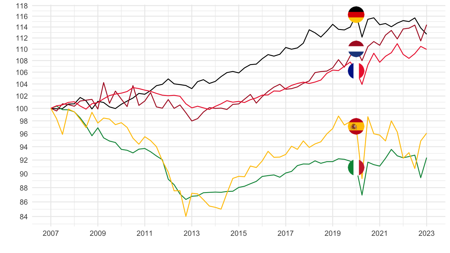
RHHGDI_INDEX - Real household gross disposable income per capita

All

Code
HH_DASH %>%
  filter(INDICATOR == "RHHGDI_INDEX",
         FREQUENCY == "Q",
         LOCATION %in% c("FRA", "DEU", "ITA", "ESP", "NLD")) %>%
  quarter_to_date %>%
  left_join(HH_DASH_var$LOCATION, by = "LOCATION") %>%
  group_by(LOCATION) %>%
  arrange(date) %>%
  mutate(obsValue = 100*obsValue/obsValue[1]) %>%
  left_join(colors, by = c("Location" = "country")) %>%
  ggplot + geom_line(aes(x = date, y = obsValue, color = color)) +
  scale_color_identity() + theme_minimal() + xlab("") + ylab("") + add_5flags +
  scale_x_date(breaks = seq.Date(from = as.Date("2007-01-01"), to = Sys.Date(), by = "2 years"),
               labels = date_format("%Y")) +
  theme(legend.position = c(0.35, 0.85),
        legend.title = element_blank()) +
  scale_y_log10(breaks = seq(10, 300, 2))

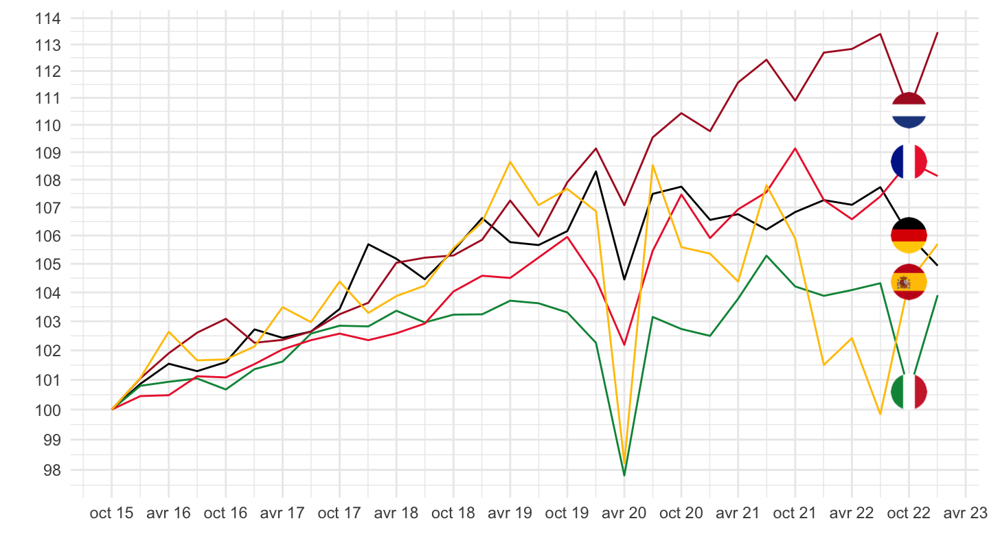
2015-

Code
HH_DASH %>%
  filter(INDICATOR == "RHHGDI_INDEX",
         FREQUENCY == "Q",
         LOCATION %in% c("FRA", "DEU", "ITA", "ESP", "NLD")) %>%
  quarter_to_date %>%
  left_join(HH_DASH_var$LOCATION, by = "LOCATION") %>%
  filter(date >= as.Date("2015-10-01")) %>%
  group_by(LOCATION) %>%
  arrange(date) %>%
  mutate(obsValue = 100*obsValue/obsValue[1]) %>%
  left_join(colors, by = c("Location" = "country")) %>%
  ggplot + geom_line(aes(x = date, y = obsValue, color = color)) +
  scale_color_identity() + theme_minimal() + xlab("") + ylab("") + add_5flags +
  scale_x_date(breaks = seq.Date(from = as.Date("2014-10-01"), to = Sys.Date(), by = "6 months"),
               labels = date_format("%b %y")) +
  theme(legend.position = c(0.35, 0.85),
        legend.title = element_blank()) +
  scale_y_log10(breaks = seq(10, 300, 1))

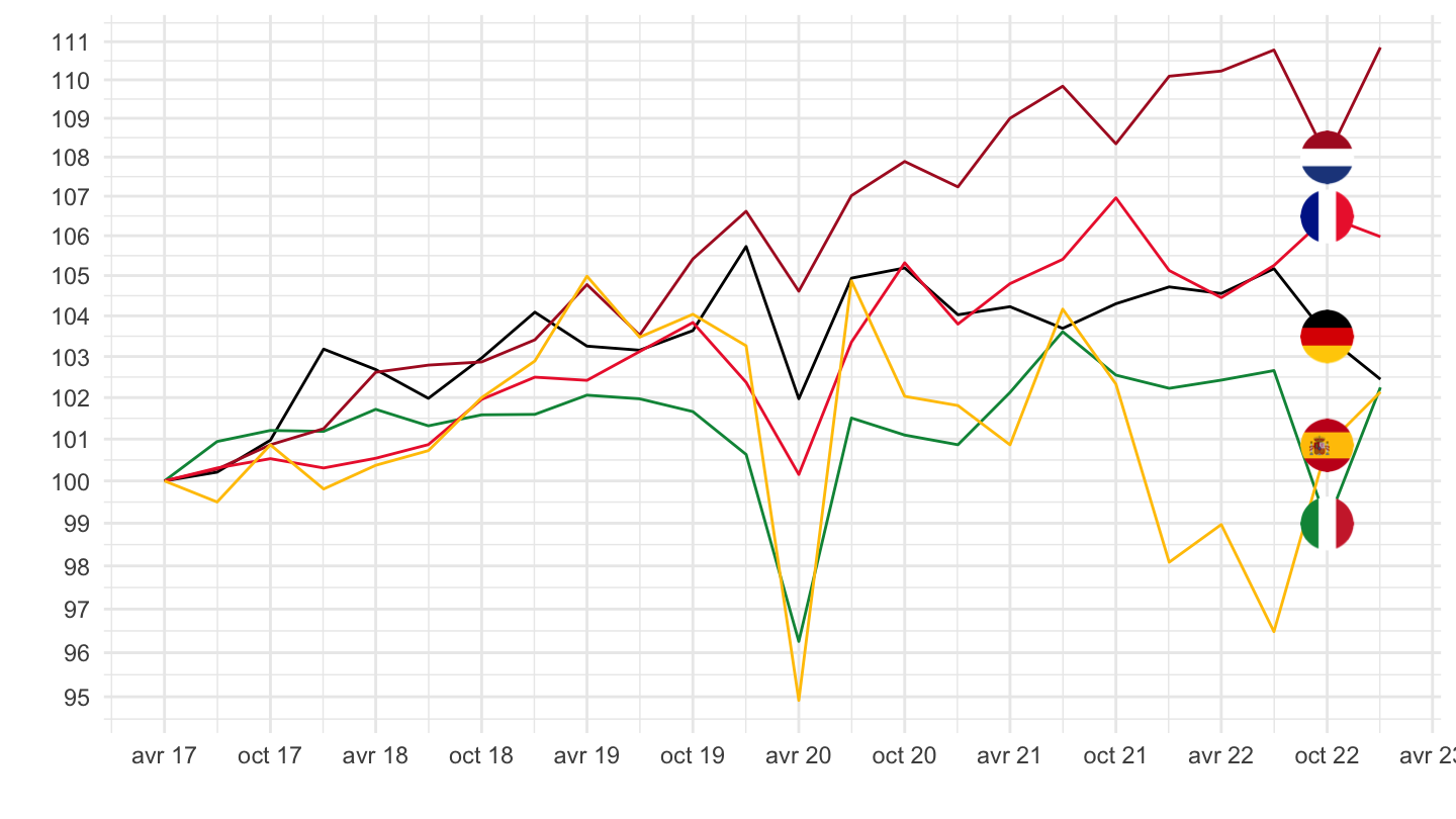
2017-

Code
HH_DASH %>%
  filter(INDICATOR == "RHHGDI_INDEX",
         FREQUENCY == "Q",
         LOCATION %in% c("FRA", "DEU", "ITA", "ESP", "NLD")) %>%
  quarter_to_date %>%
  left_join(HH_DASH_var$LOCATION, by = "LOCATION") %>%
  filter(date >= as.Date("2017-04-01")) %>%
  group_by(LOCATION) %>%
  arrange(date) %>%
  mutate(obsValue = 100*obsValue/obsValue[1]) %>%
  left_join(colors, by = c("Location" = "country")) %>%
  ggplot + geom_line(aes(x = date, y = obsValue, color = color)) +
  scale_color_identity() + theme_minimal() + xlab("") + ylab("") + add_5flags +
  scale_x_date(breaks = seq.Date(from = as.Date("2017-04-01"), to = Sys.Date(), by = "6 months"),
               labels = date_format("%b %y")) +
  theme(legend.position = c(0.35, 0.85),
        legend.title = element_blank()) +
  scale_y_log10(breaks = seq(10, 300, 1))

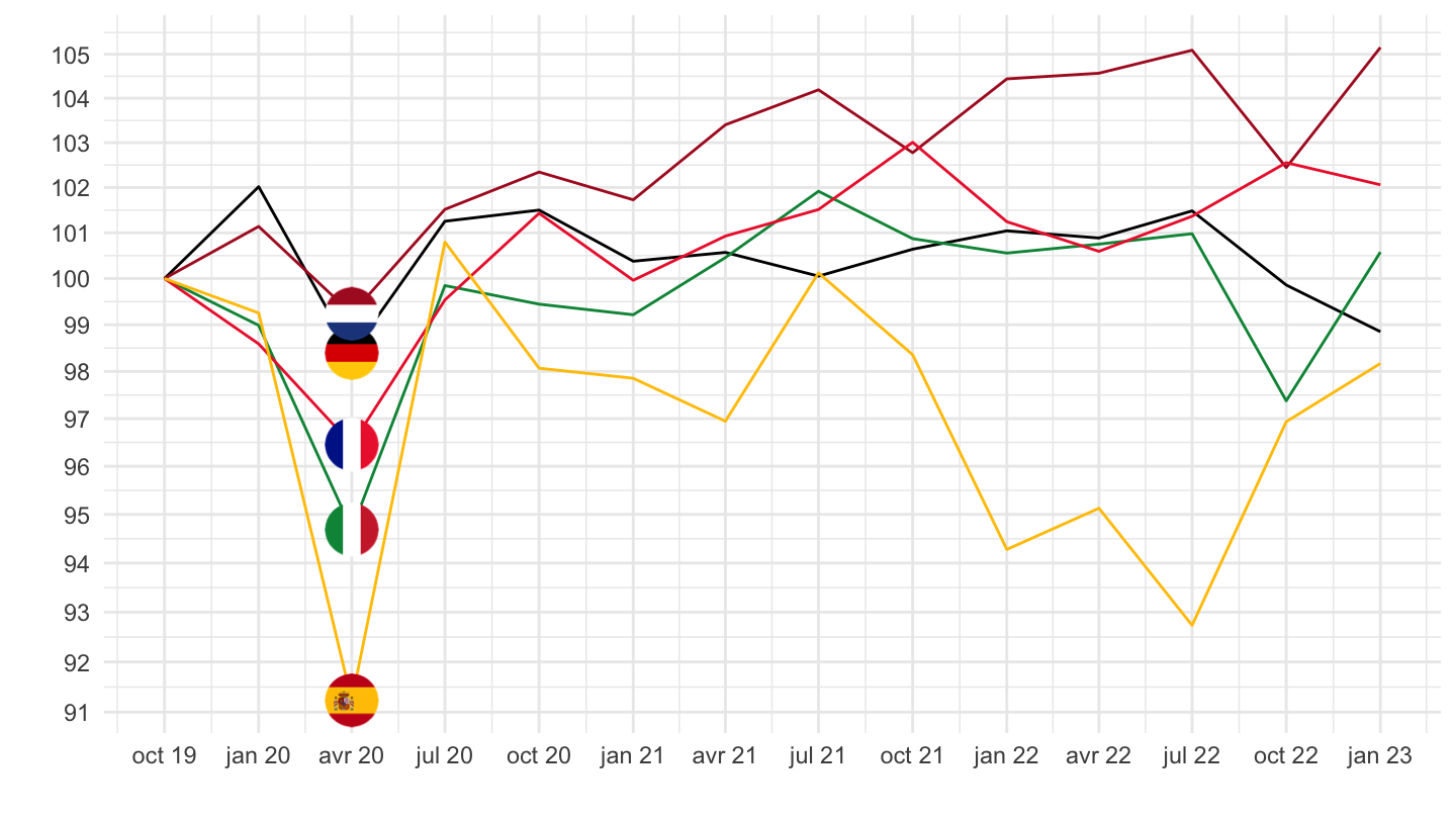
2019-

Code
HH_DASH %>%
  filter(INDICATOR == "RHHGDI_INDEX",
         FREQUENCY == "Q",
         LOCATION %in% c("FRA", "DEU", "ITA", "ESP", "NLD")) %>%
  quarter_to_date %>%
  left_join(HH_DASH_var$LOCATION, by = "LOCATION") %>%
  filter(date >= as.Date("2019-10-01")) %>%
  group_by(LOCATION) %>%
  arrange(date) %>%
  mutate(obsValue = 100*obsValue/obsValue[1]) %>%
  left_join(colors, by = c("Location" = "country")) %>%
  ggplot + geom_line(aes(x = date, y = obsValue, color = color)) +
  scale_color_identity() + theme_minimal() + xlab("") + ylab("") + add_5flags +
  scale_x_date(breaks = seq.Date(from = as.Date("2019-10-01"), to = Sys.Date(), by = "3 months"),
               labels = date_format("%b %y")) +
  theme(legend.position = c(0.35, 0.85),
        legend.title = element_blank()) +
  scale_y_log10(breaks = seq(10, 300, 1))

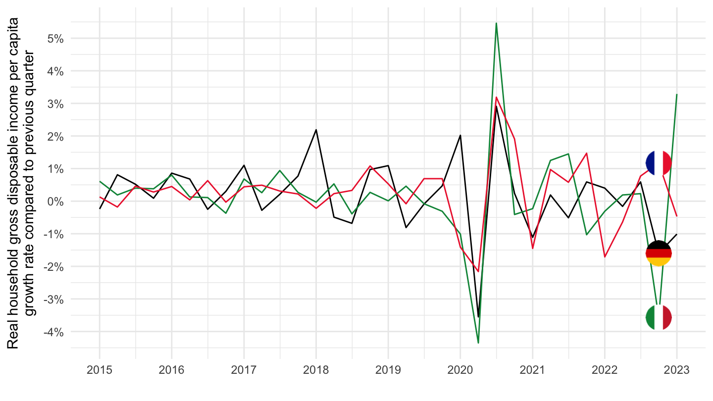
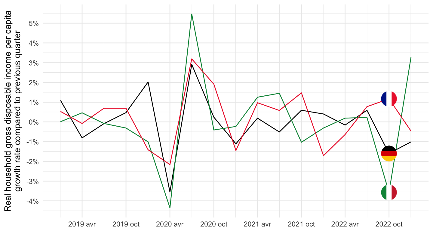
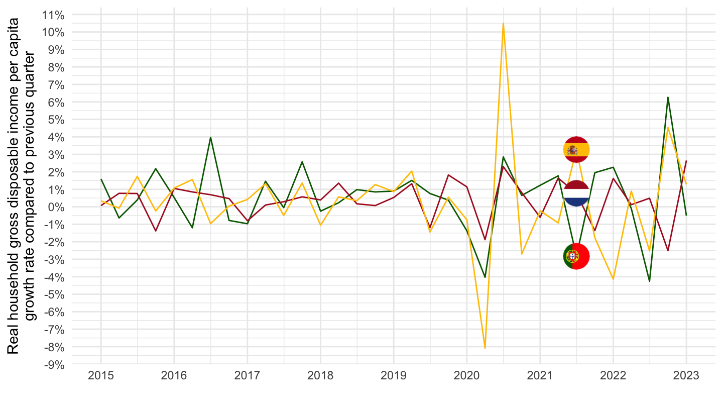
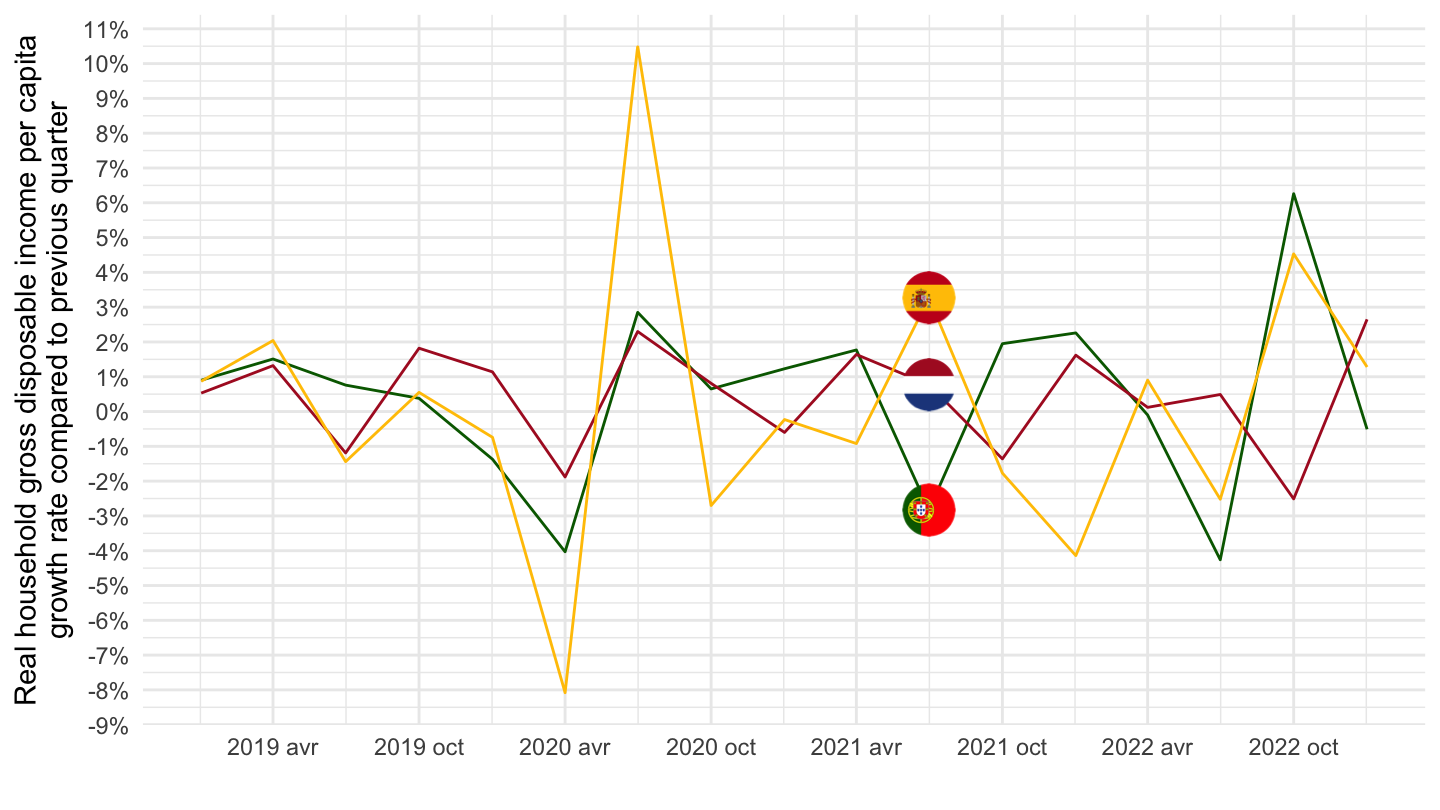
RHHGDI - Real household gross disposable income per capita, growth rate compared to previous quarter

Table: 2022-Q2, 2022-Q1

Code
HH_DASH %>%
  filter(INDICATOR == "RHHGDI",
         obsTime %in% c("2022-Q2", "2022-Q1")) %>%
  select_if(~ n_distinct(.) > 1) %>%
  spread(obsTime, obsValue) %>%
  left_join(HH_DASH_var$LOCATION, by = "LOCATION") %>%
  select(LOCATION, Location, everything()) %>%
  mutate(`2022-Q1+Q2` = `2022-Q1` + `2022-Q2`) %>%
  arrange(`2022-Q1+Q2`) %>%
  mutate(Flag = gsub(" ", "-", str_to_lower(Location)),
         Flag = paste0('<img src="../../icon/flag/vsmall/', Flag, '.png" alt="Flag">')) %>%
  select(Flag, everything()) %>%
  {if (is_html_output()) datatable(., filter = 'top', rownames = F, escape = F) else .}

Table: 2022-Q2, 2022-Q1, 2021-Q4

Code
HH_DASH %>%
  filter(INDICATOR == "RHHGDI",
         obsTime %in% c("2022-Q2", "2022-Q1", "2021-Q4")) %>%
  select_if(~ n_distinct(.) > 1) %>%
  spread(obsTime, obsValue) %>%
  left_join(HH_DASH_var$LOCATION, by = "LOCATION") %>%
  select(LOCATION, Location, everything()) %>%
  mutate(`2022-Q1+Q2` = `2022-Q1` + `2022-Q2`) %>%
  arrange(`2022-Q1+Q2`) %>%
  mutate(Flag = gsub(" ", "-", str_to_lower(Location)),
         Flag = paste0('<img src="../../icon/flag/vsmall/', Flag, '.png" alt="Flag">')) %>%
  select(Flag, everything()) %>%
  {if (is_html_output()) datatable(., filter = 'top', rownames = F, escape = F) else .}

France, Germany, Italy

2015-

Code
HH_DASH %>%
  filter(INDICATOR == "RHHGDI",
         FREQUENCY == "Q",
         LOCATION %in% c("FRA", "DEU", "ITA")) %>%
  quarter_to_date %>%
  filter(date >= as.Date("2015-01-01")) %>%
  left_join(HH_DASH_var$LOCATION, by = "LOCATION") %>%
  mutate(Location = ifelse(LOCATION == "EA19", "Europe", Location)) %>%
  left_join(colors, by = c("Location" = "country")) %>%
  mutate(color = ifelse(LOCATION == "EA19", color2, color)) %>%
  group_by(Location) %>%
  mutate(obsValue = obsValue/100) %>%
  ggplot(.) + geom_line(aes(x = date, y = obsValue, color = color)) + 
  scale_color_identity() + theme_minimal() + add_3flags +
  scale_x_date(breaks = seq(1920, 2025, 1) %>% paste0("-01-01") %>% as.Date,
               labels = date_format("%Y")) + 
  scale_y_continuous(breaks = 0.01*seq(-30, 30, 1),
                labels = percent_format(a = 1)) + 
  ylab("Real household gross disposable income per capita\ngrowth rate compared to previous quarter") + xlab("")

2019-

Code
HH_DASH %>%
  filter(INDICATOR == "RHHGDI",
         FREQUENCY == "Q",
         LOCATION %in% c("FRA", "DEU", "ITA")) %>%
  quarter_to_date %>%
  filter(date >= as.Date("2019-01-01")) %>%
  left_join(HH_DASH_var$LOCATION, by = "LOCATION") %>%
  left_join(colors, by = c("Location" = "country")) %>%
  group_by(Location) %>%
  mutate(obsValue = obsValue/100) %>%
  ggplot(.) + geom_line(aes(x = date, y = obsValue, color = color)) + 
  scale_color_identity() + theme_minimal() + add_3flags +
  scale_x_date(breaks = "6 months",
               labels = date_format("%Y %b")) + 
  scale_y_continuous(breaks = 0.01*seq(-30, 30, 1),
                labels = percent_format(a = 1)) + 
  ylab("Real household gross disposable income per capita\ngrowth rate compared to previous quarter") + xlab("")

Spain, Netherlands, Portugal

2015-

Code
HH_DASH %>%
  filter(INDICATOR == "RHHGDI",
         FREQUENCY == "Q",
         LOCATION %in% c("ESP", "NLD", "PRT")) %>%
  quarter_to_date %>%
  filter(date >= as.Date("2015-01-01")) %>%
  left_join(HH_DASH_var$LOCATION, by = "LOCATION") %>%
  mutate(Location = ifelse(LOCATION == "EA19", "Europe", Location)) %>%
  left_join(colors, by = c("Location" = "country")) %>%
  mutate(color = ifelse(LOCATION == "EA19", color2, color)) %>%
  group_by(Location) %>%
  mutate(obsValue = obsValue/100) %>%
  ggplot(.) + geom_line(aes(x = date, y = obsValue, color = color)) + 
  scale_color_identity() + theme_minimal() + add_3flags +
  scale_x_date(breaks = seq(1920, 2025, 1) %>% paste0("-01-01") %>% as.Date,
               labels = date_format("%Y")) + 
  scale_y_continuous(breaks = 0.01*seq(-30, 30, 1),
                labels = percent_format(a = 1)) + 
  ylab("Real household gross disposable income per capita\ngrowth rate compared to previous quarter") + xlab("")

2019-

Code
HH_DASH %>%
  filter(INDICATOR == "RHHGDI",
         FREQUENCY == "Q",
         LOCATION %in% c("ESP", "NLD", "PRT")) %>%
  quarter_to_date %>%
  filter(date >= as.Date("2019-01-01")) %>%
  left_join(HH_DASH_var$LOCATION, by = "LOCATION") %>%
  left_join(colors, by = c("Location" = "country")) %>%
  group_by(Location) %>%
  mutate(obsValue = obsValue/100) %>%
  ggplot(.) + geom_line(aes(x = date, y = obsValue, color = color)) + 
  scale_color_identity() + theme_minimal() + add_3flags +
  scale_x_date(breaks = "6 months",
               labels = date_format("%Y %b")) + 
  scale_y_continuous(breaks = 0.01*seq(-30, 30, 1),
                labels = percent_format(a = 1)) + 
  ylab("Real household gross disposable income per capita\ngrowth rate compared to previous quarter") + xlab("")