Salaire moyen par tête - SMPT (données CVS)
Données - INSEE
Info
Données sur les salaires
| source | dataset | Title | .html | .rData |
|---|---|---|---|---|
| insee | t_salaire_val | Salaire moyen par tête - SMPT (données CVS) | 2026-07-23 | 2026-02-27 |
| dares | les-indices-de-salaire-de-base | Les indices de salaire de base | 2026-07-20 | 2026-05-21 |
| insee | CNA-2014-RDB | Revenu et pouvoir d’achat des ménages | 2026-07-23 | 2026-07-23 |
| insee | CNT-2014-CSI | Comptes de secteurs institutionnels | 2026-07-23 | 2026-07-22 |
| insee | ECRT2023 | Emploi, chômage, revenus du travail - Edition 2023 | 2026-07-23 | 2023-06-30 |
| insee | INDICE-TRAITEMENT-FP | Indice de traitement brut dans la fonction publique de l'État | 2026-07-23 | 2026-07-23 |
| insee | SALAIRES-ACEMO | Indices trimestriels de salaires dans le secteur privé - Résultats par secteur d’activité | 2026-07-23 | 2026-07-23 |
| insee | SALAIRES-ACEMO-2017 | Indices trimestriels de salaires dans le secteur privé | 2026-07-23 | 2026-07-23 |
| insee | SALAIRES-ANNUELS | Salaires annuels | 2026-07-23 | 2026-07-23 |
| insee | T_2101 | 2.101 – Revenu disponible brut des ménages et évolution du pouvoir d'achat par personne, par ménage et par unité de consommation (En milliards euros et %) | 2026-07-23 | 2025-12-14 |
| insee | T_7401 | 7.401 – Compte des ménages (S14) (En milliards d'euros) | 2026-07-23 | 2025-12-14 |
| insee | if230 | Séries longues sur les salaires dans le secteur privé | 2026-07-23 | 2021-12-04 |
| insee | ir_salaires_SL_23_csv | NA | NA | NA |
| insee | ir_salaires_SL_csv | NA | NA | NA |
Structure
Bibliographie
Français
“Mesurer”le” pouvoir d’achat”, F. Geerolf, Document de travail, Juillet 2024. [pdf]
“Inflation en France: IPC ou IPCH ?”, F. Geerolf, Document de travail, Juillet 2024. [pdf]
“La taxe inflationniste, le pouvoir d’achat, le taux d’épargne et le déficit public”, F. Geerolf, Document de travail, Juillet 2024. [pdf]
variable
Code
t_salaire_val %>%
  group_by(variable) %>%
  summarise(Nobs = n()) %>%
  arrange(-Nobs) %>%
print_table_conditional| variable | Nobs |
|---|---|
| (DE) à (C5) | 308 |
| (DE) à (MN), (RU) | 308 |
| (GZ) à (MN), (RU) | 308 |
| AZ | 308 |
| C | 308 |
| C1 | 308 |
| C2 | 308 |
| C3 | 308 |
| C4 | 308 |
| C5 | 308 |
| DE | 308 |
| FZ | 308 |
| GZ | 308 |
| HZ | 308 |
| IZ | 308 |
| JZ | 308 |
| KZ | 308 |
| LZ | 308 |
| MN | 308 |
| OQ | 308 |
| RU | 308 |
| TOTAL | 308 |
date
Code
t_salaire_val %>%
  group_by(date) %>%
  summarise(Nobs = n()) %>%
  arrange(desc(date)) %>%
  print_table_conditional()
2021, Trimestre 3
Code
t_salaire_val %>%
  filter(date %in% c(as.Date("2023-01-01"), as.Date("2011-07-01"))) %>%
  spread(date, value) %>%
  mutate(evolution = 100*((`2023-01-01`/`2011-07-01`)^(1/10)-1)) %>%
  arrange(-`2023-01-01`) %>%
print_table_conditional()| variable | 2011-07-01 | 2023-01-01 | evolution |
|---|---|---|---|
| JZ | 12601.01 | 16504.45 | 2.7352708 |
| C4 | 11463.30 | 15042.06 | 2.7542434 |
| C2 | 13343.81 | 15025.41 | 1.1939732 |
| KZ | 11147.65 | 14848.03 | 2.9078610 |
| C3 | 10570.17 | 12633.49 | 1.7991465 |
| DE | 10228.44 | 12160.50 | 1.7452640 |
| LZ | 9999.18 | 11780.56 | 1.6529894 |
| C5 | 9067.98 | 11268.37 | 2.1962722 |
| (DE) à (C5) | 9034.70 | 11105.33 | 2.0849624 |
| MN | 8809.12 | 11048.58 | 2.2909928 |
| C | 8917.09 | 10991.16 | 2.1132357 |
| FZ | 8486.51 | 10504.59 | 2.1562631 |
| (DE) à (MN), (RU) | 8410.74 | 10483.09 | 2.2269752 |
| (GZ) à (MN), (RU) | 8249.82 | 10351.17 | 2.2950212 |
| TOTAL | 7851.68 | 9812.49 | 2.2543197 |
| HZ | 8202.63 | 9445.75 | 1.4211037 |
| GZ | 7305.37 | 9094.34 | 2.2145914 |
| OQ | 6745.87 | 8470.71 | 2.3029565 |
| C1 | 6522.67 | 8206.46 | 2.3229482 |
| RU | 6267.56 | 7689.43 | 2.0656404 |
| IZ | 5848.39 | 7153.78 | 2.0351778 |
| AZ | 6218.63 | 5968.86 | -0.4090976 |
Valeurs en Euros
KZ, JZ, C4
All
Code
t_salaire_val %>%
  filter(variable %in% c("KZ", "JZ", "C4")) %>%
  group_by(variable) %>%
  ggplot() + ylab("Salaire moyen par tête - SMPT") + xlab("") + theme_minimal() +
  geom_line(aes(x = date, y = value, color = variable)) +
  scale_x_date(breaks = seq(1920, 2100, 5) %>% paste0("-01-01") %>% as.Date,
               labels = date_format("%Y")) +
  theme(legend.position = c(0.7, 0.2),
        legend.title = element_blank()) +
  scale_y_log10(breaks = 1000*seq(1, 300, 1),
                     labels = dollar_format(accuracy = 1, su = "€", pre = "")) +
  geom_label_repel(data = . %>% filter(date == max(date)),
             aes(x = date, y = value, color = variable, label = round(value, 1)))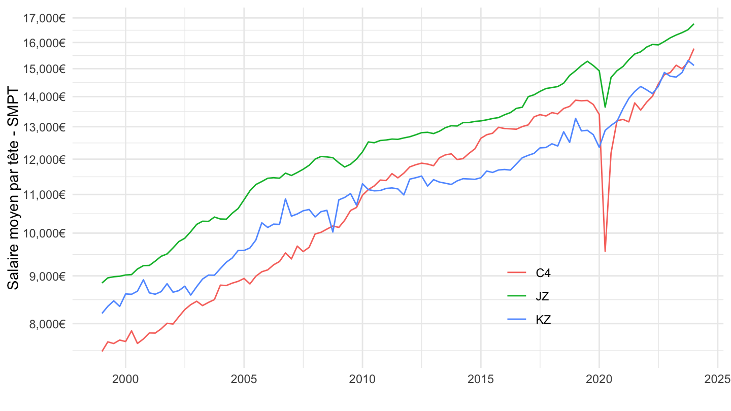
1990-
Code
t_salaire_val %>%
  filter(variable %in% c("KZ", "JZ", "C4"),
         date >= as.Date("1990-01-01")) %>%
  group_by(variable) %>%
  ggplot() + ylab("Salaire moyen par tête - SMPT") + xlab("") + theme_minimal() +
  geom_line(aes(x = date, y = value, color = variable)) +
  scale_x_date(breaks = seq(1920, 2100, 2) %>% paste0("-01-01") %>% as.Date,
               labels = date_format("%Y")) +
  theme(legend.position = c(0.7, 0.2),
        legend.title = element_blank()) +
  scale_y_log10(breaks = 1000*seq(1, 300, 1),
                     labels = dollar_format(accuracy = 1, su = "€", pre = "")) +
  geom_label_repel(data = . %>% filter(date == max(date)),
             aes(x = date, y = value, color = variable, label = round(value, 1)))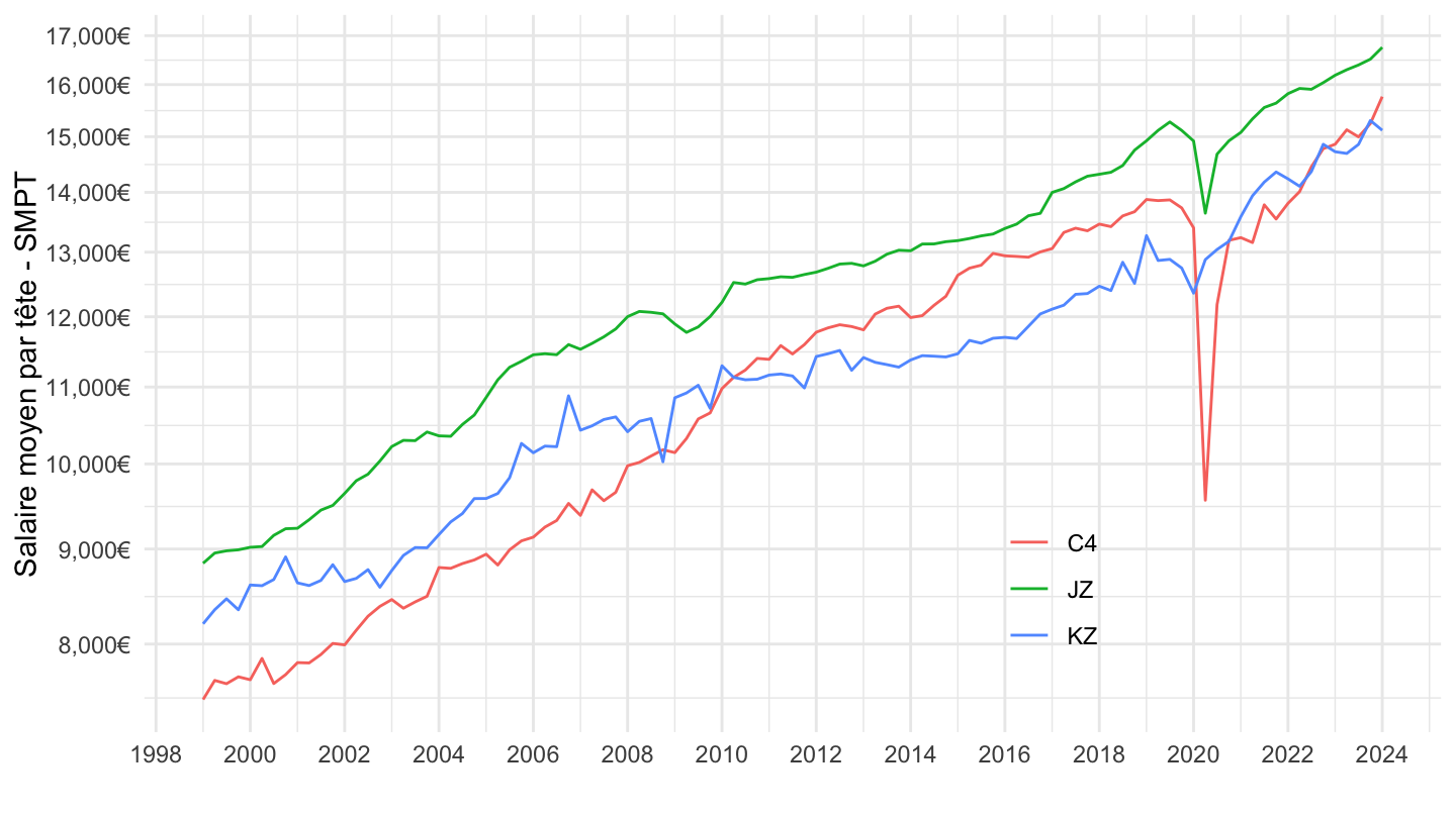
2017T2-
Code
t_salaire_val %>%
  filter(variable %in% c("KZ", "JZ", "C4"),
         date >= as.Date("2017-04-01")) %>%
  group_by(variable) %>%
  mutate(value = 100*value/value[date == as.Date("2017-04-01")]) %>%
  ggplot() + ylab("") + xlab("") + theme_minimal() +
  geom_line(aes(x = date, y = value, color = variable)) +
  scale_x_date(breaks = seq(1920, 2100, 1) %>% paste0("-01-01") %>% as.Date,
               labels = date_format("%Y")) +
  theme(legend.position = c(0.7, 0.2),
        legend.title = element_blank()) +
  scale_y_log10(breaks = seq(10, 300, 2),
                     labels = dollar_format(accuracy = 1, prefix = "")) +
  geom_label_repel(data = . %>% filter(date == max(date)),
             aes(x = date, y = value, color = variable, label = round(value, 1)))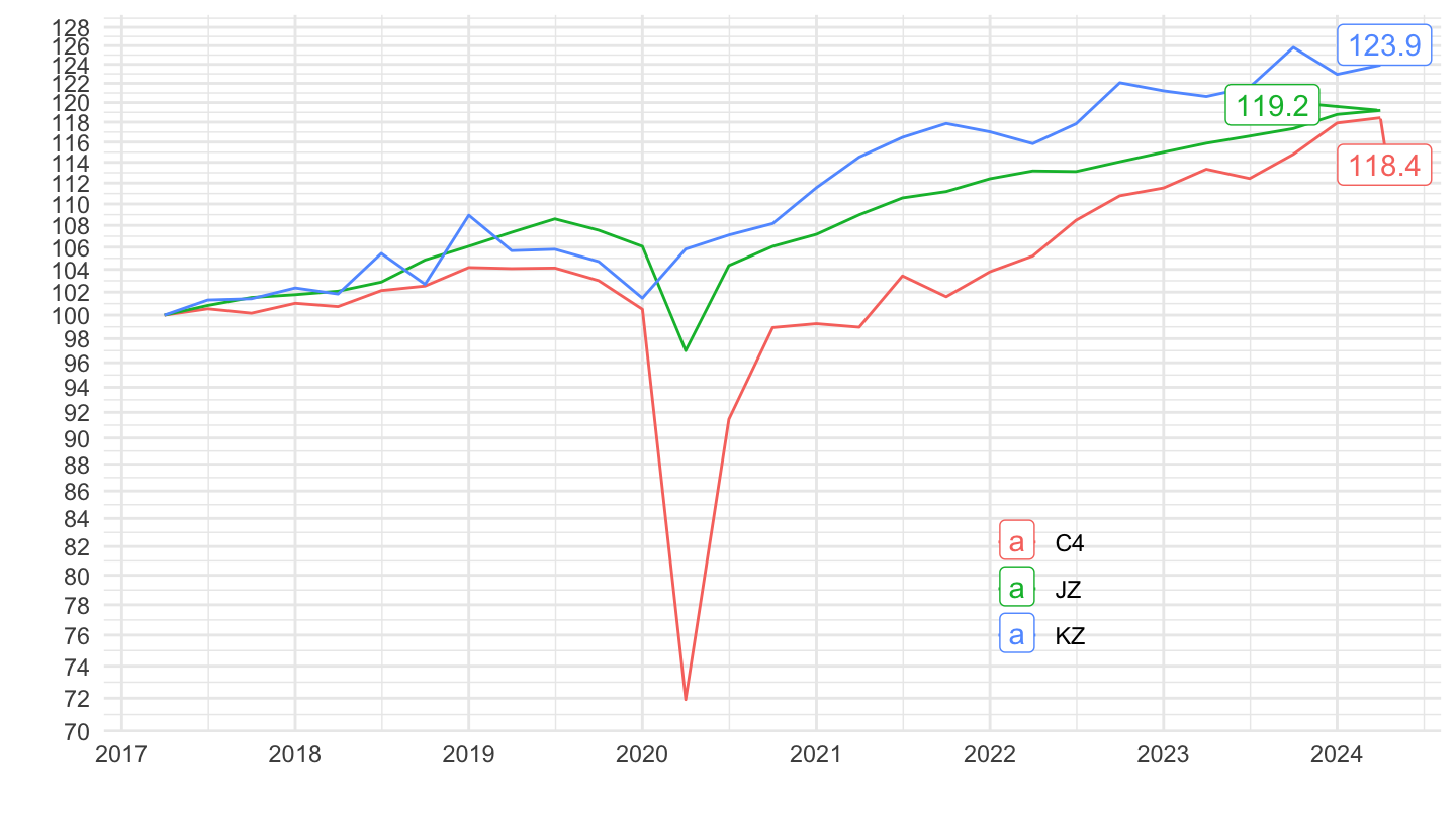
C2, C3, C4, C5
All
Code
t_salaire_val %>%
  filter(variable %in% c("C2", "C3", "C4", "C5")) %>%
  group_by(variable) %>%
  ggplot() + ylab("Salaire moyen par tête - SMPT") + xlab("") + theme_minimal() +
  geom_line(aes(x = date, y = value, color = variable)) +
  scale_x_date(breaks = seq(1920, 2100, 5) %>% paste0("-01-01") %>% as.Date,
               labels = date_format("%Y")) +
  theme(legend.position = c(0.7, 0.2),
        legend.title = element_blank()) +
  scale_y_log10(breaks = 1000*seq(1, 300, 1),
                     labels = dollar_format(accuracy = 1, su = "€", pre = "")) +
  geom_label_repel(data = . %>% filter(date == max(date)),
             aes(x = date, y = value, color = variable, label = round(value, 1)))
1990-
Code
t_salaire_val %>%
  filter(variable %in% c("C2", "C3", "C4", "C5"),
         date >= as.Date("1990-01-01")) %>%
  group_by(variable) %>%
  ggplot() + ylab("Salaire moyen par tête - SMPT") + xlab("") + theme_minimal() +
  geom_line(aes(x = date, y = value, color = variable)) +
  scale_x_date(breaks = seq(1920, 2100, 2) %>% paste0("-01-01") %>% as.Date,
               labels = date_format("%Y")) +
  theme(legend.position = c(0.7, 0.2),
        legend.title = element_blank()) +
  scale_y_log10(breaks = 1000*seq(1, 300, 1),
                     labels = dollar_format(accuracy = 1, su = "€", pre = "")) +
  geom_label_repel(data = . %>% filter(date == max(date)),
             aes(x = date, y = value, color = variable, label = round(value, 1)))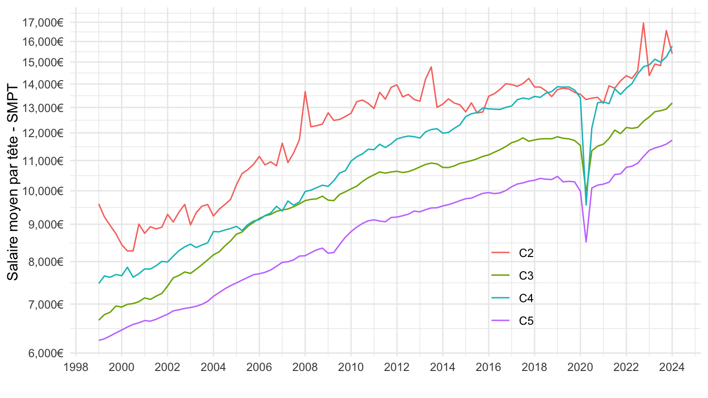
2017T2-
Code
t_salaire_val %>%
  filter(variable %in% c("C2", "C3", "C4", "C5"),
         date >= as.Date("2017-04-01")) %>%
  group_by(variable) %>%
  mutate(value = 100*value/value[date == as.Date("2017-04-01")]) %>%
  ggplot() + ylab("") + xlab("") + theme_minimal() +
  geom_line(aes(x = date, y = value, color = variable)) +
  scale_x_date(breaks = seq(1920, 2100, 1) %>% paste0("-01-01") %>% as.Date,
               labels = date_format("%Y")) +
  theme(legend.position = c(0.7, 0.2),
        legend.title = element_blank()) +
  scale_y_log10(breaks = seq(10, 300, 2),
                     labels = dollar_format(accuracy = 1, prefix = "")) +
  geom_label_repel(data = . %>% filter(date == max(date)),
             aes(x = date, y = value, color = variable, label = round(value, 1)))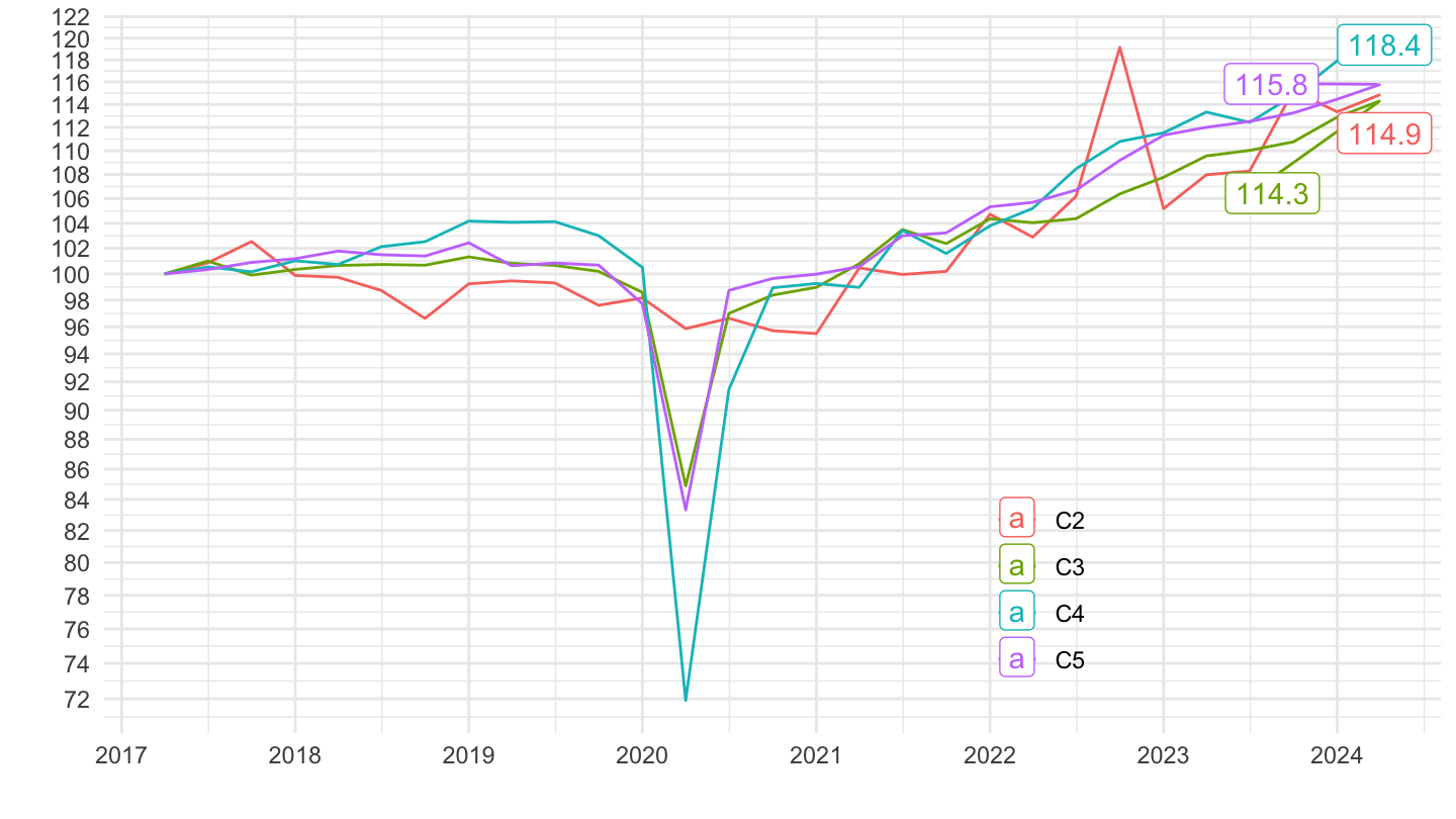
Agriculture, Industrie, Total
Value
Code
t_salaire_val %>%
  filter(variable %in% c("TOTAL", "AZ", "C"),
         date >= as.Date("1990-01-01")) %>%
  group_by(variable) %>%
  ggplot() + ylab("Salaire moyen par tête - SMPT") + xlab("") + theme_minimal() +
  geom_line(aes(x = date, y = value, color = variable)) +
  scale_x_date(breaks = seq(1920, 2100, 2) %>% paste0("-01-01") %>% as.Date,
               labels = date_format("%Y")) +
  theme(legend.position = c(0.7, 0.2),
        legend.title = element_blank()) +
  scale_y_log10(breaks = 1000*seq(1, 300, 1),
                     labels = dollar_format(accuracy = 1, su = "€", pre = "")) +
  geom_label_repel(data = . %>% filter(date == max(date)),
             aes(x = date, y = value, color = variable, label = round(value, 1)))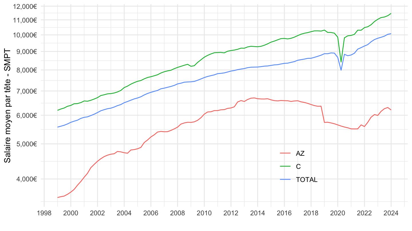
1990-
Code
t_salaire_val %>%
  filter(variable %in% c("TOTAL", "AZ", "C"),
         date >= as.Date("1990-01-01")) %>%
  group_by(variable) %>%
  mutate(value = 100*value/value[date == as.Date("1990-01-01")]) %>%
  ggplot() + ylab("") + xlab("") + theme_minimal() +
  geom_line(aes(x = date, y = value, color = variable)) +
  scale_x_date(breaks = seq(1920, 2100, 2) %>% paste0("-01-01") %>% as.Date,
               labels = date_format("%Y")) +
  theme(legend.position = c(0.7, 0.2),
        legend.title = element_blank()) +
  scale_y_log10(breaks = seq(10, 300, 10),
                     labels = dollar_format(accuracy = 1, prefix = "")) +
  geom_label_repel(data = . %>% filter(date == max(date)),
             aes(x = date, y = value, color = variable, label = round(value, 1)))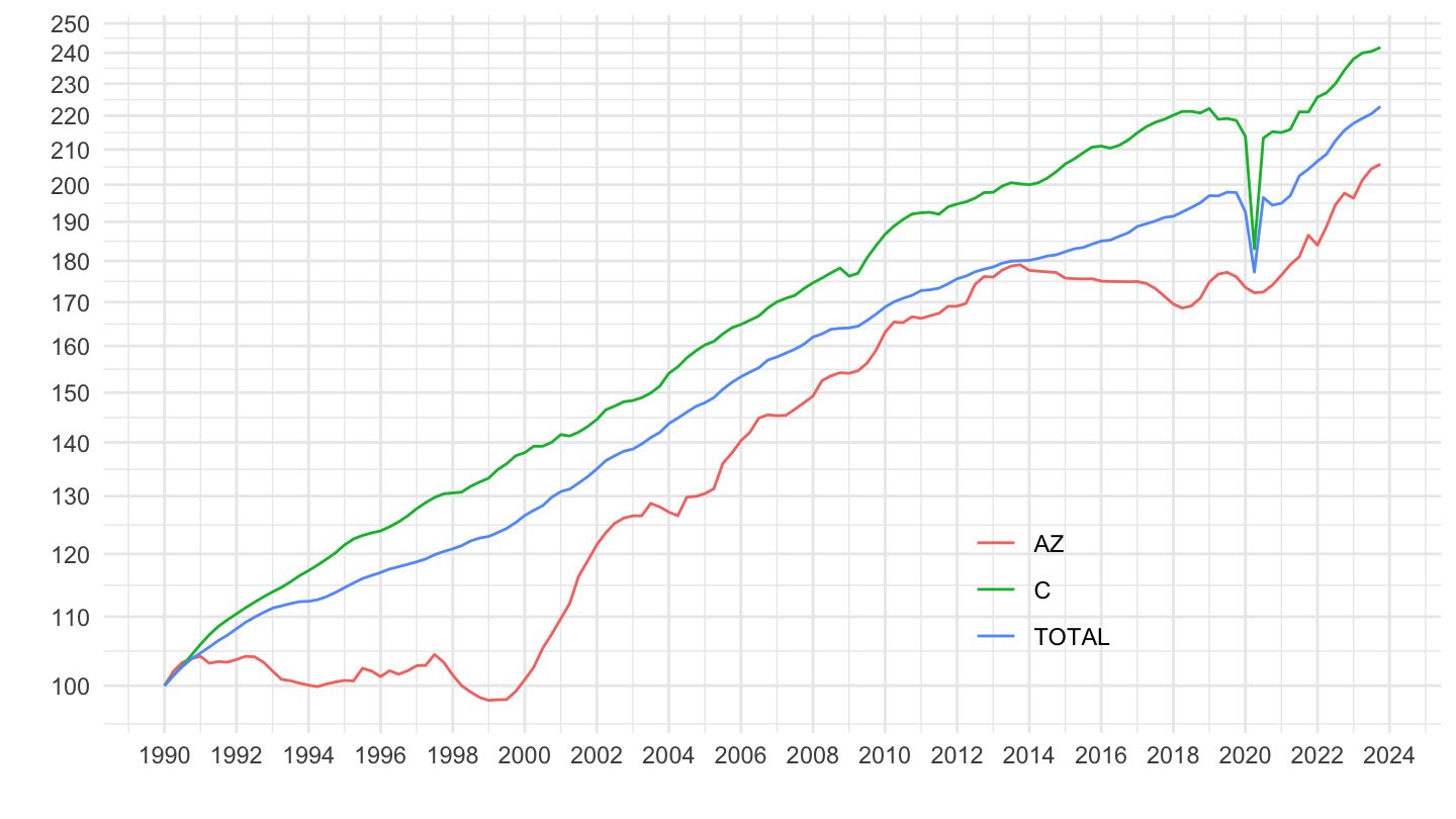
1996-
Code
t_salaire_val %>%
  filter(variable %in% c("TOTAL", "AZ", "C"),
         date >= as.Date("1996-01-01")) %>%
  group_by(variable) %>%
  mutate(value = 100*value/value[date == as.Date("1996-01-01")]) %>%
  ggplot() + ylab("") + xlab("") + theme_minimal() +
  geom_line(aes(x = date, y = value, color = variable)) +
  scale_x_date(breaks = seq(1920, 2100, 2) %>% paste0("-01-01") %>% as.Date,
               labels = date_format("%Y")) +
  theme(legend.position = c(0.7, 0.2),
        legend.title = element_blank()) +
  scale_y_log10(breaks = seq(10, 300, 10),
                     labels = dollar_format(accuracy = 1, prefix = "")) +
  geom_label_repel(data = . %>% filter(date == max(date)),
             aes(x = date, y = value, color = variable, label = round(value, 1)))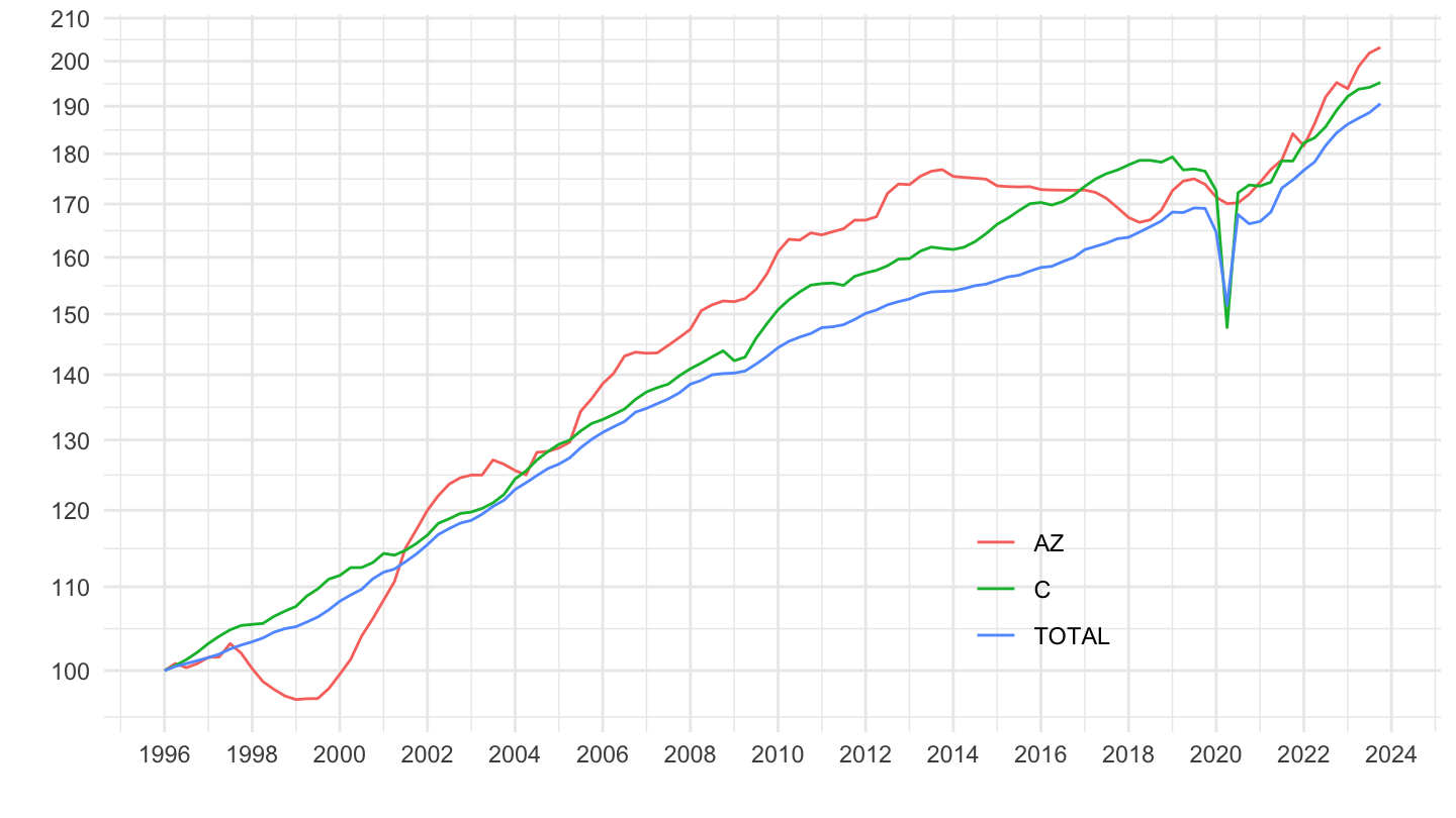
2012-
Code
t_salaire_val %>%
  filter(variable %in% c("TOTAL", "AZ", "C"),
         date >= as.Date("2012-01-01")) %>%
  group_by(variable) %>%
  mutate(value = 100*value/value[date == as.Date("2012-01-01")]) %>%
  ggplot() + ylab("") + xlab("") + theme_minimal() +
  geom_line(aes(x = date, y = value, color = variable)) +
  scale_x_date(breaks = seq(1920, 2100, 1) %>% paste0("-01-01") %>% as.Date,
               labels = date_format("%Y")) +
  theme(legend.position = c(0.7, 0.2),
        legend.title = element_blank()) +
  scale_y_log10(breaks = seq(10, 300, 2),
                     labels = dollar_format(accuracy = 1, prefix = "")) +
  geom_label_repel(data = . %>% filter(date == max(date)),
             aes(x = date, y = value, color = variable, label = round(value, 1)))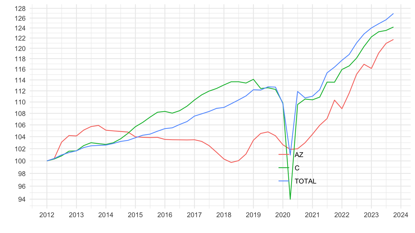
2017-
Code
t_salaire_val %>%
  filter(variable %in% c("TOTAL", "AZ", "C"),
         date >= as.Date("2017-01-01")) %>%
  group_by(variable) %>%
  mutate(value = 100*value/value[date == as.Date("2017-01-01")]) %>%
  ggplot() + ylab("") + xlab("") + theme_minimal() +
  geom_line(aes(x = date, y = value, color = variable)) +
  scale_x_date(breaks = seq(1920, 2100, 1) %>% paste0("-01-01") %>% as.Date,
               labels = date_format("%Y")) +
  theme(legend.position = c(0.7, 0.2),
        legend.title = element_blank()) +
  scale_y_log10(breaks = seq(10, 300, 2),
                     labels = dollar_format(accuracy = 1, prefix = "")) +
  geom_label_repel(data = . %>% filter(date == max(date)),
             aes(x = date, y = value, color = variable, label = round(value, 1)))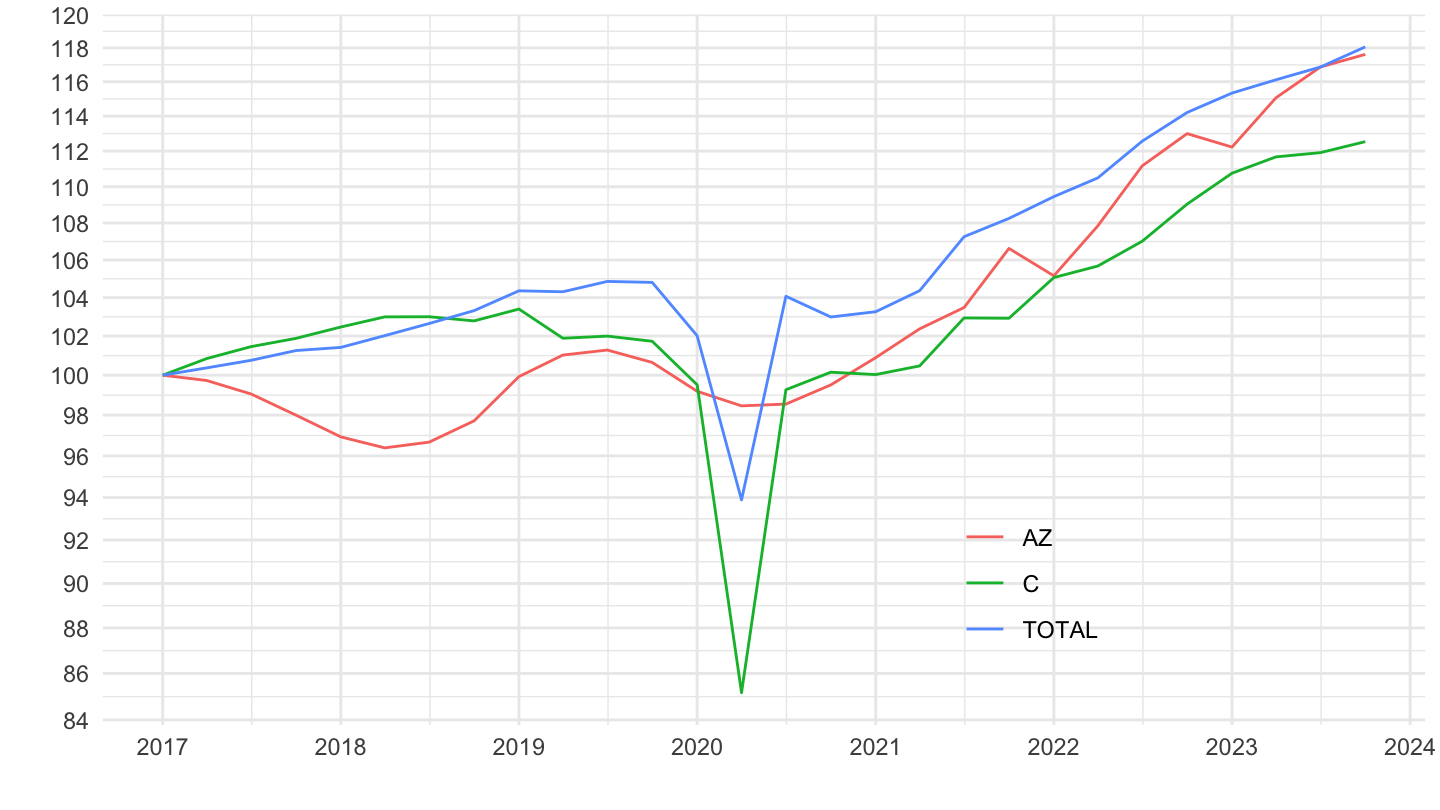
2017T1-
Code
t_salaire_val %>%
  filter(variable %in% c("TOTAL", "AZ", "C"),
         date >= as.Date("2017-01-01")) %>%
  group_by(variable) %>%
  mutate(value = 100*value/value[date == as.Date("2017-01-01")]) %>%
  ggplot() + ylab("") + xlab("") + theme_minimal() +
  geom_line(aes(x = date, y = value, color = variable)) +
  scale_x_date(breaks = seq(1920, 2100, 1) %>% paste0("-01-01") %>% as.Date,
               labels = date_format("%Y")) +
  theme(legend.position = c(0.7, 0.2),
        legend.title = element_blank()) +
  scale_y_log10(breaks = seq(10, 300, 2),
                     labels = dollar_format(accuracy = 1, prefix = "")) +
  geom_label_repel(data = . %>% filter(date == max(date)),
             aes(x = date, y = value, color = variable, label = round(value, 1)))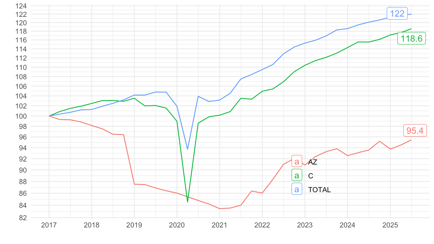
2017T2-
Code
t_salaire_val %>%
  filter(variable %in% c("TOTAL", "AZ", "C"),
         date >= as.Date("2017-04-01")) %>%
  group_by(variable) %>%
  mutate(value = 100*value/value[date == as.Date("2017-04-01")]) %>%
  ggplot() + ylab("") + xlab("") + theme_minimal() +
  geom_line(aes(x = date, y = value, color = variable)) +
  scale_x_date(breaks = seq(1920, 2100, 1) %>% paste0("-01-01") %>% as.Date,
               labels = date_format("%Y")) +
  theme(legend.position = c(0.7, 0.2),
        legend.title = element_blank()) +
  scale_y_log10(breaks = seq(10, 300, 2),
                     labels = dollar_format(accuracy = 1, prefix = "")) +
  geom_label_repel(data = . %>% filter(date == max(date)),
             aes(x = date, y = value, color = variable, label = round(value, 1)))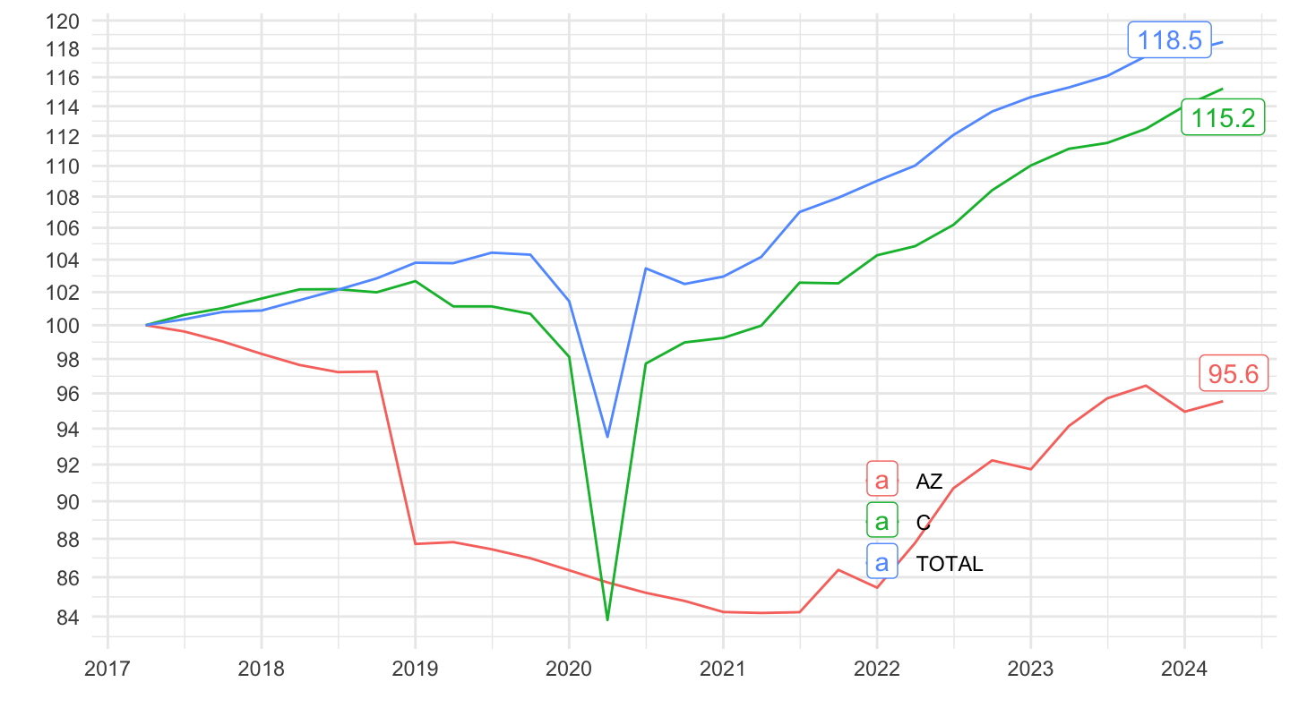
2019T4-
Code
t_salaire_val %>%
  filter(variable %in% c("TOTAL", "AZ", "C"),
         date >= as.Date("2019-10-01")) %>%
  group_by(variable) %>%
  mutate(value = 100*value/value[date == as.Date("2019-10-01")]) %>%
  ggplot() + ylab("") + xlab("") + theme_minimal() +
  geom_line(aes(x = date, y = value, color = variable)) +
  scale_x_date(breaks = seq(1920, 2100, 1) %>% paste0("-01-01") %>% as.Date,
               labels = date_format("%Y")) +
  theme(legend.position = c(0.7, 0.2),
        legend.title = element_blank()) +
  scale_y_log10(breaks = seq(10, 300, 2),
                     labels = dollar_format(accuracy = 1, prefix = "")) +
  geom_label_repel(data = . %>% filter(date == max(date)),
             aes(x = date, y = value, color = variable, label = round(value, 1)))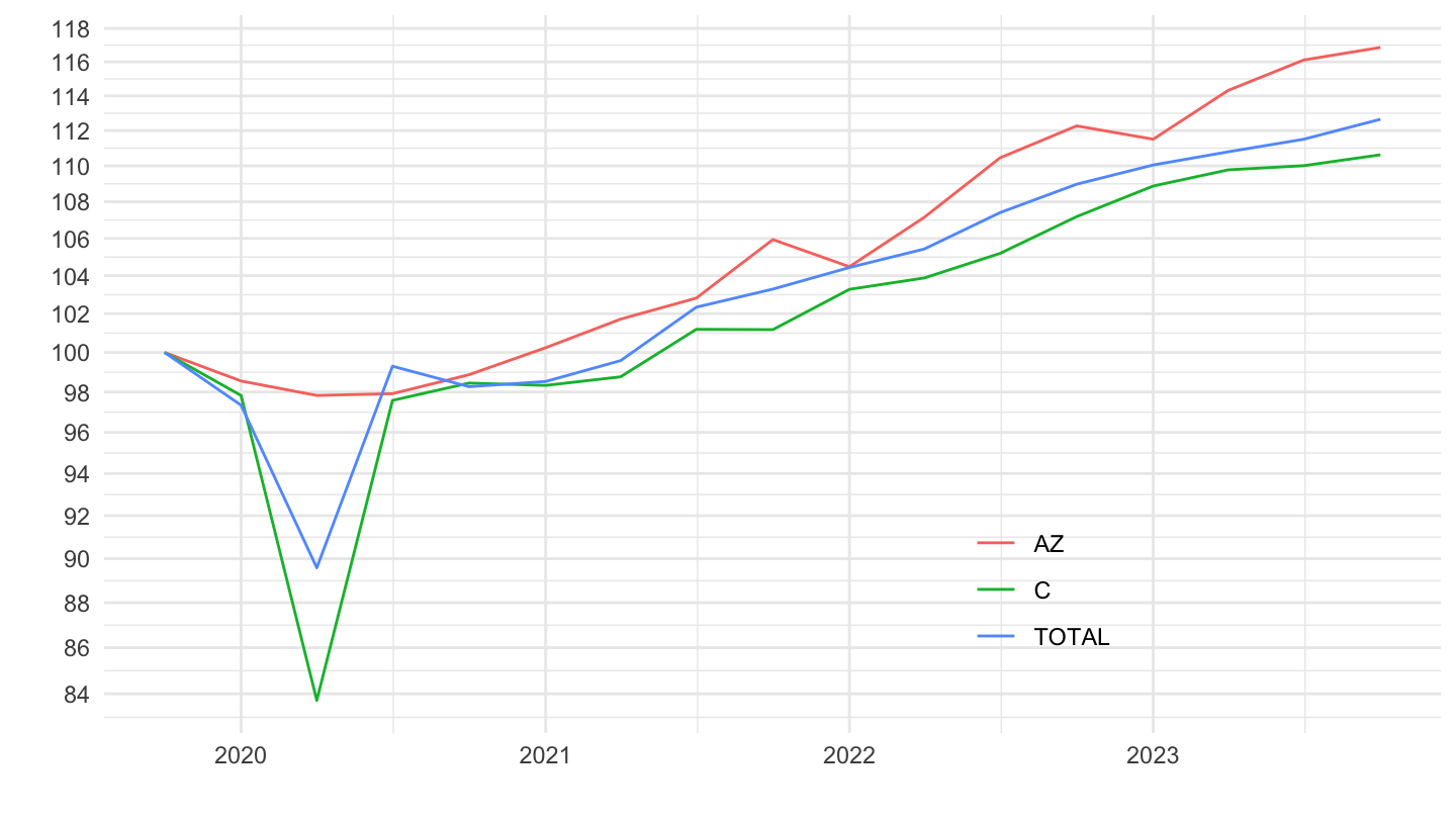
2021T3-
Code
df <- t_salaire_val %>%
  filter(variable %in% c("TOTAL", "AZ", "C"),
         date >= as.Date("2021-07-01")) %>%
  group_by(variable) %>%
  arrange(date) %>%
  mutate(value = 100*value/value[1]) %>%
  date_to_yearqtr()

ggplot(data = df) + ylab("") + xlab("") + theme_minimal() +
  geom_line(aes(x = date, y = value, color = variable)) +
  scale_x_yearqtr(labels = date_format("%Y T%q"),
                  breaks = seq(from = min(df$date), to = max(df$date), by = 0.25)) +
  theme(legend.position = c(0.7, 0.2),
        legend.title = element_blank(),
        axis.text.x = element_text(angle = 45, vjust = 1, hjust = 1)) +
  scale_y_log10(breaks = seq(10, 300, 1),
                     labels = dollar_format(accuracy = 1, prefix = "")) +
  geom_label_repel(data = . %>% filter(date == max(date)),
             aes(x = date, y = value, color = variable, label = round(value, 1)))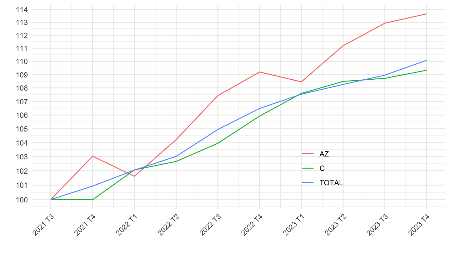
2021T4-
Code
df <- t_salaire_val %>%
  filter(variable %in% c("TOTAL", "AZ", "C"),
         date >= as.Date("2021-10-01")) %>%
  group_by(variable) %>%
  arrange(date) %>%
  mutate(value = 100*value/value[1]) %>%
  date_to_yearqtr()

ggplot(data = df) + ylab("") + xlab("") + theme_minimal() +
  geom_line(aes(x = date, y = value, color = variable)) +
  scale_x_yearqtr(labels = date_format("%Y T%q"),
                  breaks = seq(from = min(df$date), to = max(df$date), by = 0.25)) +
  theme(legend.position = c(0.7, 0.2),
        legend.title = element_blank(),
        axis.text.x = element_text(angle = 45, vjust = 1, hjust = 1)) +
  scale_y_log10(breaks = seq(10, 300, 1),
                     labels = dollar_format(accuracy = 1, prefix = "")) +
  geom_label_repel(data = . %>% filter(date == max(date)),
             aes(x = date, y = value, color = variable, label = round(value, 1)))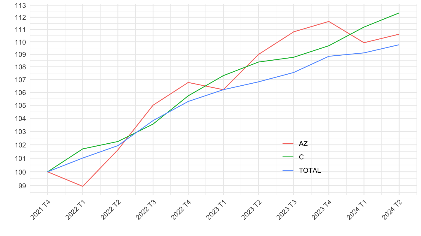
Services Marchands, Total, Non Marchands
1990-
Code
t_salaire_val %>%
  filter(variable %in% c("TOTAL", "OQ", "(GZ) à (MN), (RU)"),
         date >= as.Date("1990-01-01")) %>%
  group_by(variable) %>%
  mutate(value = 100*value/value[date == as.Date("1990-01-01")]) %>%
  ggplot() + ylab("") + xlab("") + theme_minimal() +
  geom_line(aes(x = date, y = value, color = variable)) +
  scale_x_date(breaks = seq(1920, 2100, 2) %>% paste0("-01-01") %>% as.Date,
               labels = date_format("%Y")) +
  theme(legend.position = c(0.7, 0.2),
        legend.title = element_blank()) +
  scale_y_log10(breaks = seq(10, 300, 5),
                     labels = dollar_format(accuracy = 1, prefix = "")) +
  geom_label_repel(data = . %>% filter(date == max(date)),
             aes(x = date, y = value, color = variable, label = round(value, 1)))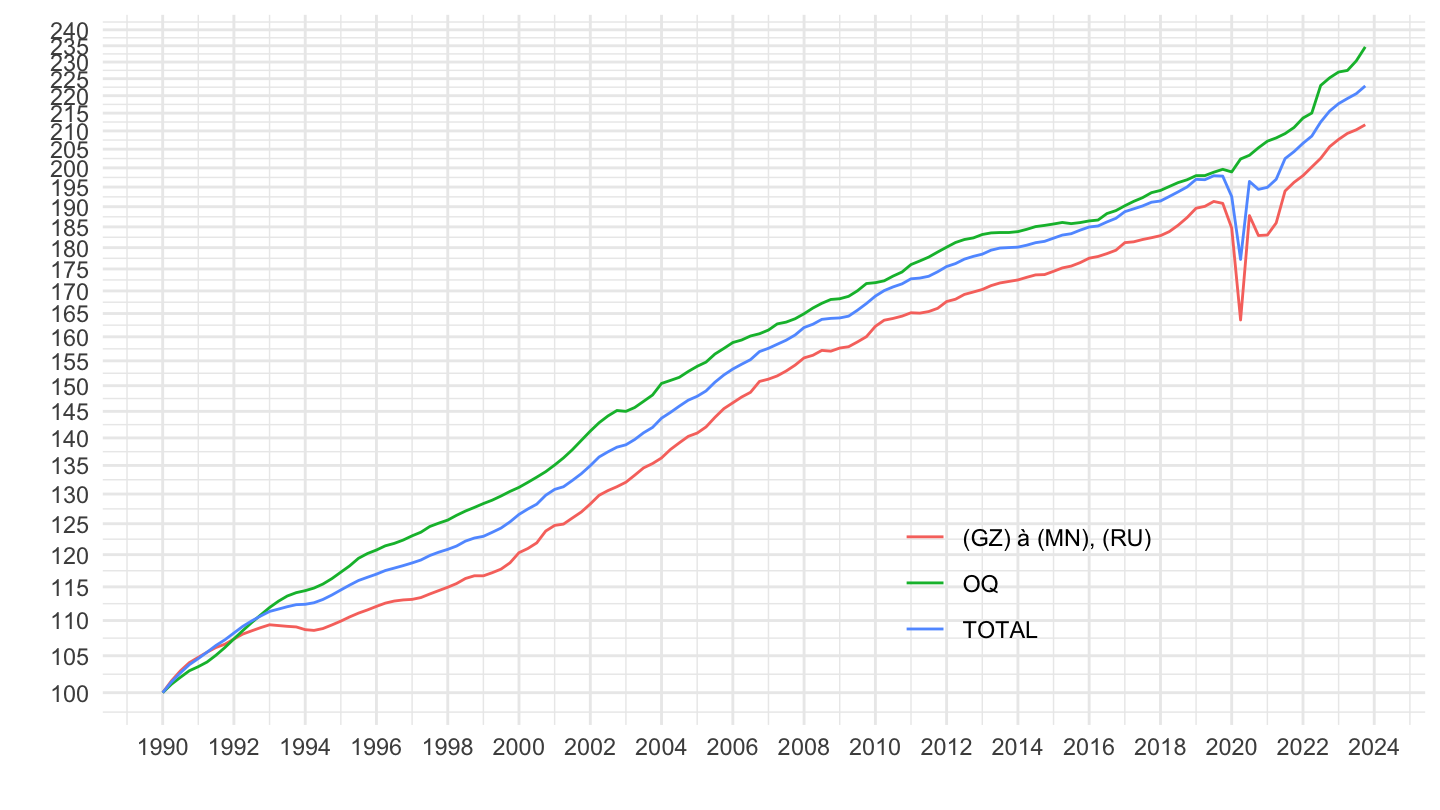
1996-
Code
t_salaire_val %>%
  filter(variable %in% c("TOTAL", "OQ", "(GZ) à (MN), (RU)"),
         date >= as.Date("1996-01-01")) %>%
  group_by(variable) %>%
  mutate(value = 100*value/value[date == as.Date("1996-01-01")]) %>%
  ggplot() + ylab("") + xlab("") + theme_minimal() +
  geom_line(aes(x = date, y = value, color = variable)) +
  scale_x_date(breaks = seq(1920, 2100, 2) %>% paste0("-01-01") %>% as.Date,
               labels = date_format("%Y")) +
  theme(legend.position = c(0.7, 0.2),
        legend.title = element_blank()) +
  scale_y_log10(breaks = seq(10, 300, 5),
                     labels = dollar_format(accuracy = 1, prefix = "")) +
  geom_label_repel(data = . %>% filter(date == max(date)),
             aes(x = date, y = value, color = variable, label = round(value, 1)))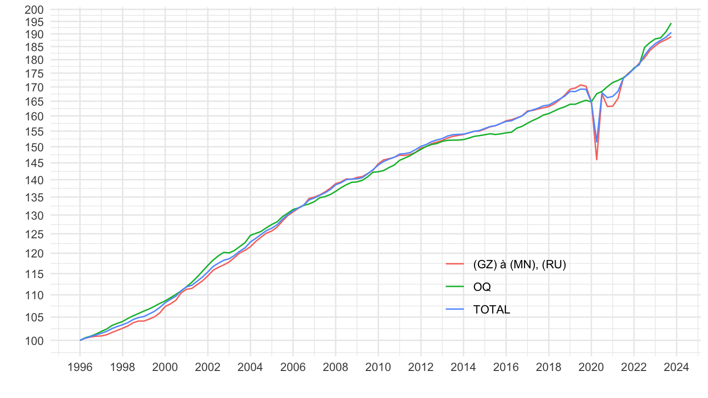
2012-
Code
t_salaire_val %>%
  filter(variable %in% c("TOTAL", "OQ", "(GZ) à (MN), (RU)"),
         date >= as.Date("2012-01-01")) %>%
  group_by(variable) %>%
  mutate(value = 100*value/value[date == as.Date("2012-01-01")]) %>%
  ggplot() + ylab("") + xlab("") + theme_minimal() +
  geom_line(aes(x = date, y = value, color = variable)) +
  scale_x_date(breaks = seq(1920, 2100, 1) %>% paste0("-01-01") %>% as.Date,
               labels = date_format("%Y")) +
  theme(legend.position = c(0.7, 0.2),
        legend.title = element_blank()) +
  scale_y_log10(breaks = seq(10, 300, 2),
                     labels = dollar_format(accuracy = 1, prefix = "")) +
  geom_label_repel(data = . %>% filter(date == max(date)),
             aes(x = date, y = value, color = variable, label = round(value, 1)))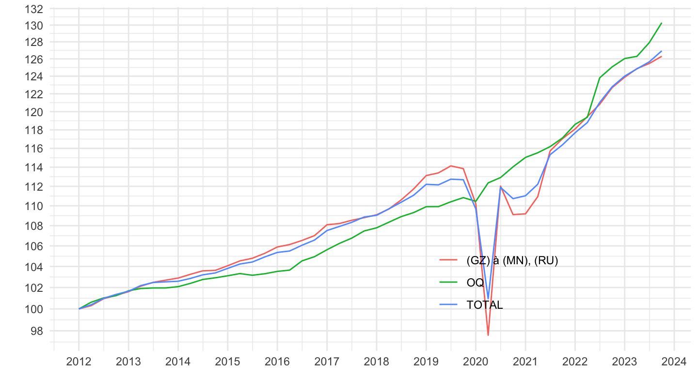
2017-
Code
df <- t_salaire_val %>%
  filter(variable %in% c("TOTAL", "OQ", "(GZ) à (MN), (RU)"),
         date >= as.Date("2017-01-01")) %>%
  group_by(variable) %>%
  arrange(date) %>%
  mutate(value = 100*value/value[1]) %>%
  date_to_yearqtr %>%
  ungroup

ggplot(data = df) + ylab("") + xlab("") + theme_minimal() +
  geom_line(aes(x = date, y = value, color = variable)) +
  scale_x_yearqtr(labels = date_format("%Y T%q"),
                  breaks = seq(from = min(df$date), to = max(df$date), by = 0.5)) +
  theme(legend.position = c(0.7, 0.2),
        legend.title = element_blank(),
        axis.text.x = element_text(angle = 45, vjust = 1, hjust = 1)) +
  scale_y_log10(breaks = seq(10, 300, 2),
                     labels = dollar_format(accuracy = 1, prefix = "")) +
  geom_label_repel(data = . %>% filter(date == max(date)),
             aes(x = date, y = value, color = variable, label = round(value, 1)))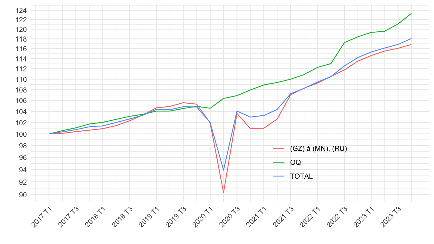
2017T1-
Code
df <- t_salaire_val %>%
  filter(variable %in% c("TOTAL", "OQ", "(GZ) à (MN), (RU)"),
         date >= as.Date("2017-01-01")) %>%
  group_by(variable) %>%
  arrange(date) %>%
  mutate(value = 100*value/value[1]) %>%
  date_to_yearqtr %>%
  ungroup

ggplot(data = df) + ylab("") + xlab("") + theme_minimal() +
  geom_line(aes(x = date, y = value, color = variable)) +
  scale_x_yearqtr(labels = date_format("%Y T%q"),
                  breaks = seq(from = min(df$date), to = max(df$date), by = 0.5)) +
  theme(legend.position = c(0.7, 0.2),
        legend.title = element_blank(),
        axis.text.x = element_text(angle = 45, vjust = 1, hjust = 1)) +
  scale_y_log10(breaks = seq(10, 300, 2),
                     labels = dollar_format(accuracy = 1, prefix = "")) +
  geom_label_repel(data = . %>% filter(date == max(date)),
             aes(x = date, y = value, color = variable, label = round(value, 1)))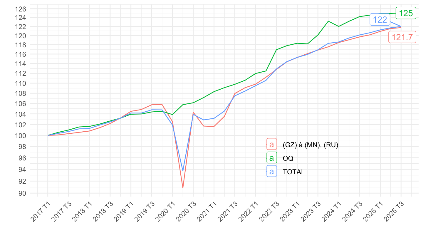
2017T2-
Code
df <- t_salaire_val %>%
  filter(variable %in% c("TOTAL", "OQ", "(GZ) à (MN), (RU)"),
         date >= as.Date("2017-04-01")) %>%
  group_by(variable) %>%
  arrange(date) %>%
  mutate(value = 100*value/value[1]) %>%
  date_to_yearqtr %>%
  ungroup

ggplot(data = df) + ylab("") + xlab("") + theme_minimal() +
  geom_line(aes(x = date, y = value, color = variable)) +
  scale_x_yearqtr(labels = date_format("%Y T%q"),
                  breaks = seq(from = min(df$date), to = max(df$date), by = 0.5)) +
  theme(legend.position = c(0.7, 0.2),
        legend.title = element_blank(),
        axis.text.x = element_text(angle = 45, vjust = 1, hjust = 1)) +
  scale_y_log10(breaks = seq(10, 300, 2),
                     labels = dollar_format(accuracy = 1, prefix = "")) +
  geom_label_repel(data = . %>% filter(date == max(date)),
             aes(x = date, y = value, color = variable, label = round(value, 1)))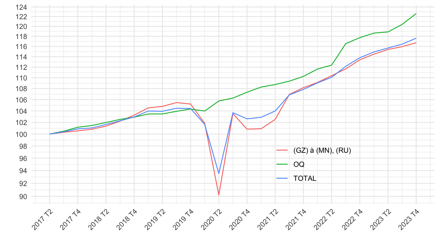
2019T4-
Code
df <- t_salaire_val %>%
  filter(variable %in% c("TOTAL", "OQ", "(GZ) à (MN), (RU)"),
         date >= as.Date("2019-10-01")) %>%
  group_by(variable) %>%
  arrange(date) %>%
  mutate(value = 100*value/value[1]) %>%
  date_to_yearqtr %>%
  ungroup

ggplot(data = df) + ylab("") + xlab("") + theme_minimal() +
  geom_line(aes(x = date, y = value, color = variable)) +
  scale_x_yearqtr(labels = date_format("%Y T%q"),
                  breaks = seq(from = min(df$date), to = max(df$date), by = 0.25)) +
  theme(legend.position = c(0.7, 0.2),
        legend.title = element_blank(),
        axis.text.x = element_text(angle = 45, vjust = 1, hjust = 1)) +
  scale_y_log10(breaks = seq(10, 300, 2),
                     labels = dollar_format(accuracy = 1, prefix = "")) +
  geom_label_repel(data = . %>% filter(date == max(date)),
             aes(x = date, y = value, color = variable, label = round(value, 1)))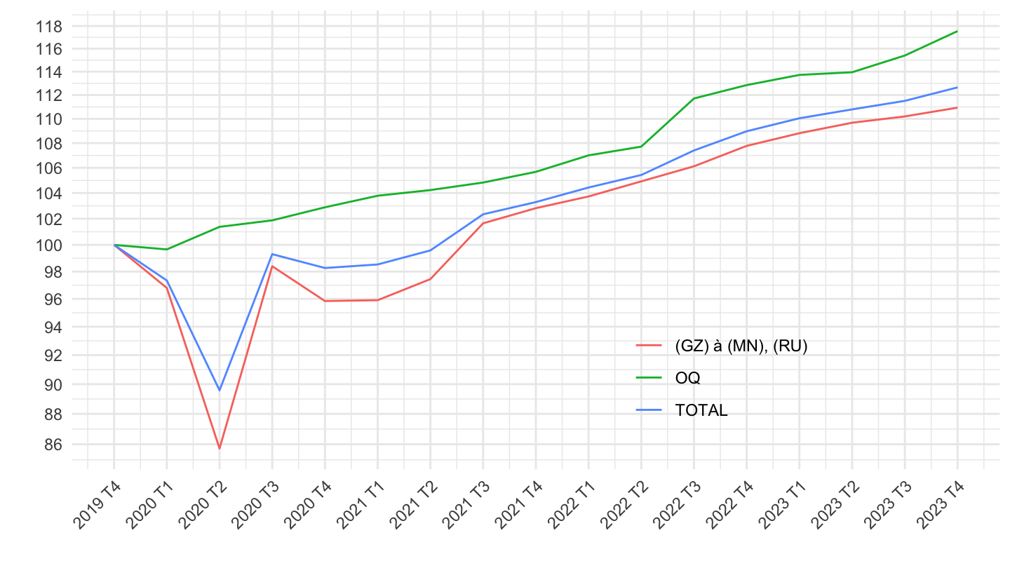
2021T2-
Code
df <- t_salaire_val %>%
  filter(variable %in% c("TOTAL", "OQ", "(GZ) à (MN), (RU)"),
         date >= as.Date("2021-04-01")) %>%
  group_by(variable) %>%
  arrange(date) %>%
  mutate(value = 100*value/value[1]) %>%
  date_to_yearqtr %>%
  ungroup

ggplot(data = df) + ylab("") + xlab("") + theme_minimal() +
  geom_line(aes(x = date, y = value, color = variable)) +
  scale_x_yearqtr(labels = date_format("%Y T%q"),
                  breaks = seq(from = min(df$date), to = max(df$date), by = 0.25)) +
  theme(legend.position = c(0.7, 0.2),
        legend.title = element_blank(),
        axis.text.x = element_text(angle = 45, vjust = 1, hjust = 1)) +
  scale_y_log10(breaks = seq(10, 300, 2),
                     labels = dollar_format(accuracy = 1, prefix = "")) +
  geom_label_repel(data = . %>% filter(date == max(date)),
             aes(x = date, y = value, color = variable, label = round(value, 1)))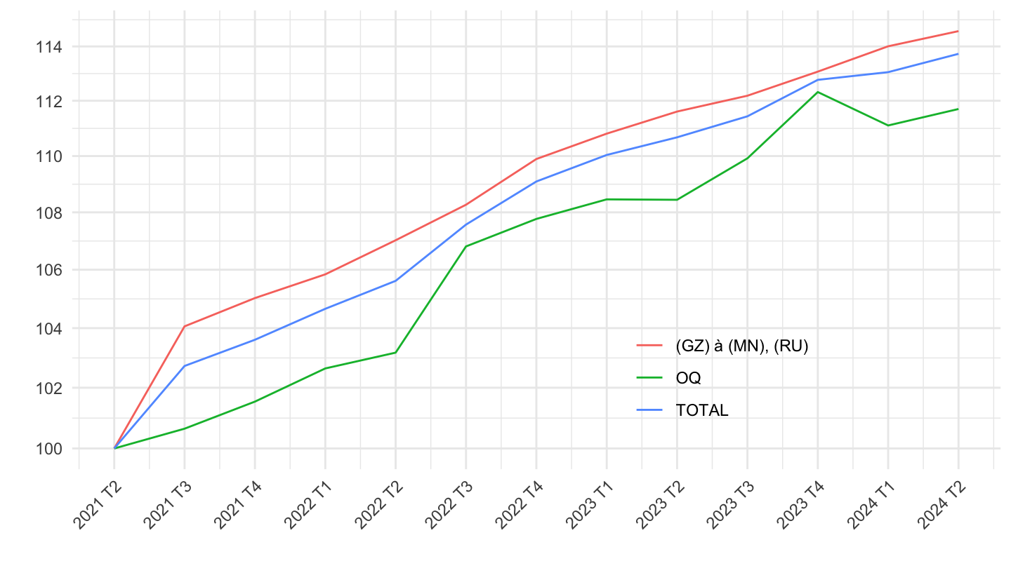
2021T3-
Code
df <- t_salaire_val %>%
  filter(variable %in% c("TOTAL", "OQ", "(GZ) à (MN), (RU)"),
         date >= as.Date("2021-07-01")) %>%
  group_by(variable) %>%
  arrange(date) %>%
  mutate(value = 100*value/value[1]) %>%
  date_to_yearqtr %>%
  ungroup

ggplot(data = df) + ylab("") + xlab("") + theme_minimal() +
  geom_line(aes(x = date, y = value, color = variable)) +
  scale_x_yearqtr(labels = date_format("%Y T%q"),
                  breaks = seq(from = min(df$date), to = max(df$date), by = 0.25)) +
  theme(legend.position = c(0.7, 0.2),
        legend.title = element_blank(),
        axis.text.x = element_text(angle = 45, vjust = 1, hjust = 1)) +
  scale_y_log10(breaks = seq(10, 300, 2),
                     labels = dollar_format(accuracy = 1, prefix = "")) +
  geom_label_repel(data = . %>% filter(date == max(date)),
             aes(x = date, y = value, color = variable, label = round(value, 1)))
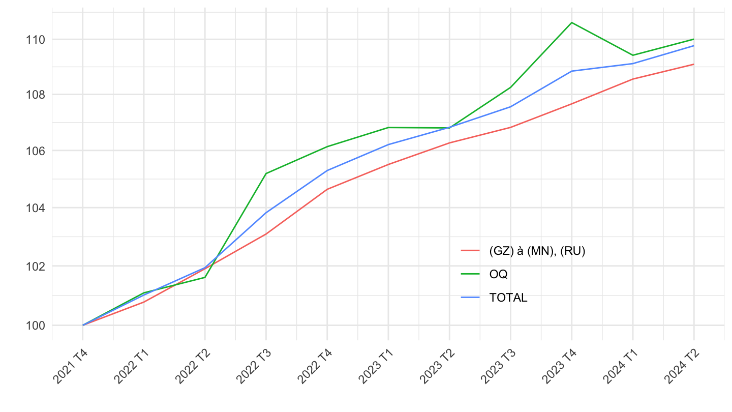
2021T4-
Nominal
Code
df <- t_salaire_val %>%
  filter(variable %in% c("TOTAL", "OQ", "(GZ) à (MN), (RU)"),
         date >= as.Date("2021-10-01")) %>%
  group_by(variable) %>%
  arrange(date) %>%
  mutate(value = 100*value/value[1]) %>%
  date_to_yearqtr %>%
  ungroup

ggplot(data = df) + ylab("") + xlab("") + theme_minimal() +
  geom_line(aes(x = date, y = value, color = variable)) +
  scale_x_yearqtr(labels = date_format("%Y T%q"),
                  breaks = seq(from = min(df$date), to = max(df$date), by = 0.25)) +
  theme(legend.position = c(0.7, 0.2),
        legend.title = element_blank(),
        axis.text.x = element_text(angle = 45, vjust = 1, hjust = 1)) +
  scale_y_log10(breaks = seq(10, 300, 2),
                     labels = dollar_format(accuracy = 1, prefix = "")) +
  geom_label_repel(data = . %>% filter(date == max(date)),
             aes(x = date, y = value, color = variable, label = round(value, 1)))