| source | dataset | Title | .html | .rData |
|---|---|---|---|---|
| insee | conso-eff-fonction | Consommation effective des ménages par fonction | 2026-07-23 | 2022-06-14 |
Consommation effective des ménages par fonction
Données - INSEE
Info
Données sur le pouvoir d’achat
| source | dataset | Title | .html | .rData |
|---|---|---|---|---|
| insee | conso-eff-fonction | Consommation effective des ménages par fonction | 2026-07-23 | 2022-06-14 |
| insee | CNA-2014-RDB | Revenu et pouvoir d’achat des ménages | 2026-07-23 | 2026-07-23 |
| insee | CNT-2014-CSI | Comptes de secteurs institutionnels | 2026-07-23 | 2026-07-22 |
| insee | T_2101 | 2.101 – Revenu disponible brut des ménages et évolution du pouvoir d'achat par personne, par ménage et par unité de consommation (En milliards euros et %) | 2026-07-23 | 2025-12-14 |
| insee | T_7401 | 7.401 – Compte des ménages (S14) (En milliards d'euros) | 2026-07-23 | 2025-12-14 |
| insee | econ-gen-revenu-dispo-pouv-achat-2 | Revenu disponible brut et pouvoir d’achat - Données annuelles | 2026-07-23 | 2026-01-11 |
| insee | reve-conso-evo-dep-pa | Évolution de la dépense et du pouvoir d’achat des ménages - Données annuelles de 1960 à 2023 | 2026-07-23 | 2024-12-11 |
| insee | reve-niv-vie-individu-activite | Niveau de vie selon l'activité - Données annuelles | 2026-07-23 | 2025-12-22 |
| insee | reve-niv-vie-pouv-achat-trim | Évolution du revenu disponible brut et du pouvoir d’achat - Données trimestrielles | 2026-07-23 | 2026-01-11 |
| insee | t_men_val | Revenu, pouvoir d'achat et comptes des ménages - Valeurs aux prix courants | 2026-07-23 | 2026-02-27 |
| insee | t_pouvachat_val | Pouvoir d'achat et ratios des comptes des ménages | 2026-07-23 | 2026-02-27 |
| insee | t_recapAgent_val | Récapitulatif des séries des comptes d'agents | 2026-07-23 | 2026-02-27 |
| insee | t_salaire_val | Salaire moyen par tête - SMPT (données CVS) | 2026-07-23 | 2026-02-27 |
| oecd | HH_DASH | Household Dashboard | 2026-07-23 | 2023-09-09 |
LAST_COMPILE
| LAST_COMPILE |
|---|
| 2026-07-24 |
Dernière
Code
`conso-eff-fonction` %>%
  group_by(year) %>%
  summarise(Nobs = n()) %>%
  arrange(desc(year)) %>%
  head(2) %>%
print_table_conditional()| year | Nobs |
|---|---|
| 2021 | 882 |
| 2020 | 882 |
Données reliées
Sources
Info
Les tableaux détaillés présentent la consommation effective des ménages depuis 1959 jusqu’à l’année du compte provisoire, déclinée aux niveaux diffusables les plus fins des nomenclatures de produits (Nomenclature agrégée), de fonction (COICOP) et de durabilité.
Pour chaque nomenclature (produit, fonction durabilité), les résultats détaillés ont le format suivant :
- Séries en niveau :
- Consommation aux prix courants (onglet M€cour), que l’on appelle aussi “en valeur” ou “en euros courants”
- Consommation en volume aux prix de l’année précédente chaînés (onglet M€2014), que l’on appelle aussi ““en volume”” ou en ““euros 2014”“. Les consommations en volume au prix de l’année précédente chaînée ne sont pas sommables. En conséquence, la somme des consommations en volume aux prix de l’année précédente chaîné des séries élémentaires constituant un niveau diffère de la consommation pour le niveau total de l’agrégat.
- Indices de prix base 100 en 2014 (onglet Iprix2014)
- Séries en évolution n/n-1 :
- Indices de valeur base 100 l’année précédente (onglet Ival)
- Indices de volume base 100 l’année précédente (onglet Ivol)
- Indices de prix base 100 l’année précédente (onglet Iprix)
- Structure des séries :
- Coefficients budgétaires aux prix courants en % (onglet Coeffcour)
variable
Code
`conso-eff-fonction` %>%
  group_by(variable) %>%
  summarise(Nobs = n()) %>%
print_table_conditional()| variable | Nobs |
|---|---|
| Coeffcour | 9261 |
| Iprix2014 | 9261 |
| Ival | 9114 |
| Ivol | 9114 |
| M€2014 | 9261 |
| M€cour | 9261 |
fonction, Fonction
Tous
Code
`conso-eff-fonction` %>%
  group_by(fonction, Fonction) %>%
  summarise(Nobs = n()) %>%
  print_table_conditional()
2-digit
Code
`conso-eff-fonction` %>%
  filter(nchar(fonction) == 2) %>%
  group_by(fonction, Fonction) %>%
  summarise(Nobs = n()) %>%
print_table_conditional()| fonction | Fonction | Nobs |
|---|---|---|
| 01 | Produits alimentaires et boissons non alcoolisées | 376 |
| 02 | Boissons alcoolisées et tabac | 376 |
| 03 | Articles d'habillement et chaussures | 376 |
| 04 | Logement, eau, gaz, électricité et autres combustibles | 376 |
| 05 | Meubles, articles de ménage et entretien courant de l'habitation | 376 |
| 06 | Santé | 376 |
| 07 | Transports | 376 |
| 08 | Communications | 376 |
| 09 | Loisirs et culture | 376 |
| 10 | Éducation | 376 |
| 11 | Hôtels, cafés et restaurants | 376 |
| 12 | Biens et services divers | 376 |
| 13 | Dépense de consommation finale individualisable des ISBLSM | 376 |
| 14 | Dépense de consommation finale individualisable des APU | 376 |
| 15 | Solde territorial | 376 |
3-digit
Code
`conso-eff-fonction` %>%
  filter(nchar(fonction) == 4) %>%
  group_by(fonction, Fonction) %>%
  summarise(Nobs = n()) %>%
  print_table_conditional()
4-digit
Code
`conso-eff-fonction` %>%
  filter(nchar(fonction) == 6) %>%
  group_by(fonction, Fonction) %>%
  summarise(Nobs = n()) %>%
  print_table_conditional()
5-digit
Code
`conso-eff-fonction` %>%
  filter(nchar(fonction) == 8) %>%
  group_by(fonction, Fonction) %>%
  summarise(Nobs = n()) %>%
print_table_conditional()| fonction | Fonction | Nobs |
|---|---|---|
| 09.2.1-2 | Autres biens durables culturels et récréatifs neufs | 376 |
| 12.1.2-3 | Appareils et produits pour soins corporels | 376 |
Autres
Code
`conso-eff-fonction` %>%
  filter(!(nchar(fonction) %in% c(2, 4, 6))) %>%
  group_by(fonction, Fonction) %>%
  summarise(Nobs = n()) %>%
print_table_conditional()| fonction | Fonction | Nobs |
|---|---|---|
| 01..12+15 | Dépense de consommation des ménages | 376 |
| 01..12+15 (HS) | Dépense de consommation des ménages hors SIFIM | 376 |
| 09.2.1-2 | Autres biens durables culturels et récréatifs neufs | 376 |
| 12.1.2-3 | Appareils et produits pour soins corporels | 376 |
| NA | Consommation effective des ménages | 376 |
year
Code
`conso-eff-fonction` %>%
  group_by(year) %>%
  summarise(Nobs = n()) %>%
  arrange(desc(year)) %>%
  print_table_conditional()
2020
Désordonné
Code
`conso-eff-fonction` %>%
  filter(variable == "M€cour") %>%
  year_to_date2 %>%
  left_join(gdp, by = "date") %>%
  filter(date == as.Date("2020-01-01")) %>%
  select(-date) %>%
  mutate(`% du PIB` = (100*value/(gdp)) %>% round(., digits = 2),
         value = round(value) %>% paste0(" Mds€")) %>%
  select(-gdp) %>%
  {if (is_html_output()) datatable(., filter = 'top', rownames = F) else .}
Ordonné
Code
`conso-eff-fonction` %>%
  filter(variable == "M€cour") %>%
  year_to_date2 %>%
  left_join(gdp, by = "date") %>%
  filter(date == as.Date("2020-01-01")) %>%
  select(-date) %>%
  arrange(-value) %>%
  mutate(`% du PIB` = (100*value/(gdp)) %>% round(., digits = 2),
         value = round(value) %>% paste0(" Mds€")) %>%
  select(-gdp) %>%
  print_table_conditional()
Loyers réels, loyers imputés
Mds €
Code
`conso-eff-fonction` %>%
  filter(variable == "M€cour") %>%
  year_to_date2 %>%
  filter(fonction %in% c("04.1", "04.2", "04.5")) %>%
  left_join(gdp, by = "date") %>%
  ggplot(.) + theme_minimal() + ylab("Consommation (Milliards€)") + xlab("") +
  geom_line(aes(x = date, y = value/1000, color = Fonction)) +
  theme(legend.title = element_blank(),
        legend.position = c(0.3, 0.91)) +
  scale_x_date(breaks = seq(1950, 2020, 5) %>% paste0("-01-01") %>% as.Date,
               labels = date_format("%Y")) +
  scale_y_continuous(breaks = seq(0, 500, 20),
                     labels = dollar_format(acc = 1, pre = "", su = " Mds€"))
% de la consommation
Code
`conso-eff-fonction` %>%
  filter(variable == "M€cour") %>%
  year_to_date2 %>%
  filter(fonction %in% c("04.1", "04.2", "04.5")) %>%
  left_join(gdp, by = "date") %>%
  ggplot(.) + theme_minimal() + ylab("Consommation (% du PIB)") + xlab("") +
  geom_line(aes(x = date, y = value/(gdp), color = Fonction)) +
  theme(legend.title = element_blank(),
        legend.position = c(0.3, 0.91)) +
  scale_x_date(breaks = seq(1950, 2020, 5) %>% paste0("-01-01") %>% as.Date,
               labels = date_format("%Y")) +

  scale_y_continuous(breaks = 0.01*seq(0, 100, 0.5),
                     labels = scales::percent_format(accuracy = 0.1))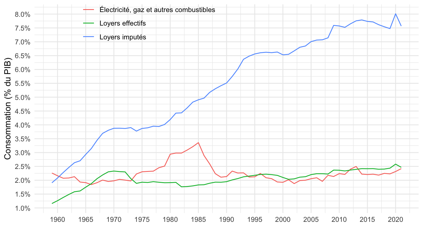
Entretien et réparation des logements
Code
`conso-eff-fonction` %>%
  filter(variable == "M€cour") %>%
  year_to_date2 %>%
  filter(fonction %in% c("04.3", "04.4")) %>%
  left_join(gdp, by = "date") %>%
  ggplot(.) + theme_minimal() + ylab("Consommation (% du PIB)") + xlab("") +
  geom_line(aes(x = date, y = value/(gdp), color = Fonction)) +
  theme(legend.title = element_blank(),
        legend.position = c(0.6, 0.2)) +
  scale_x_date(breaks = seq(1950, 2020, 5) %>% paste0("-01-01") %>% as.Date,
               labels = date_format("%Y")) +

  scale_y_continuous(breaks = 0.01*seq(0, 100, 0.1),
                     labels = scales::percent_format(accuracy = 0.1))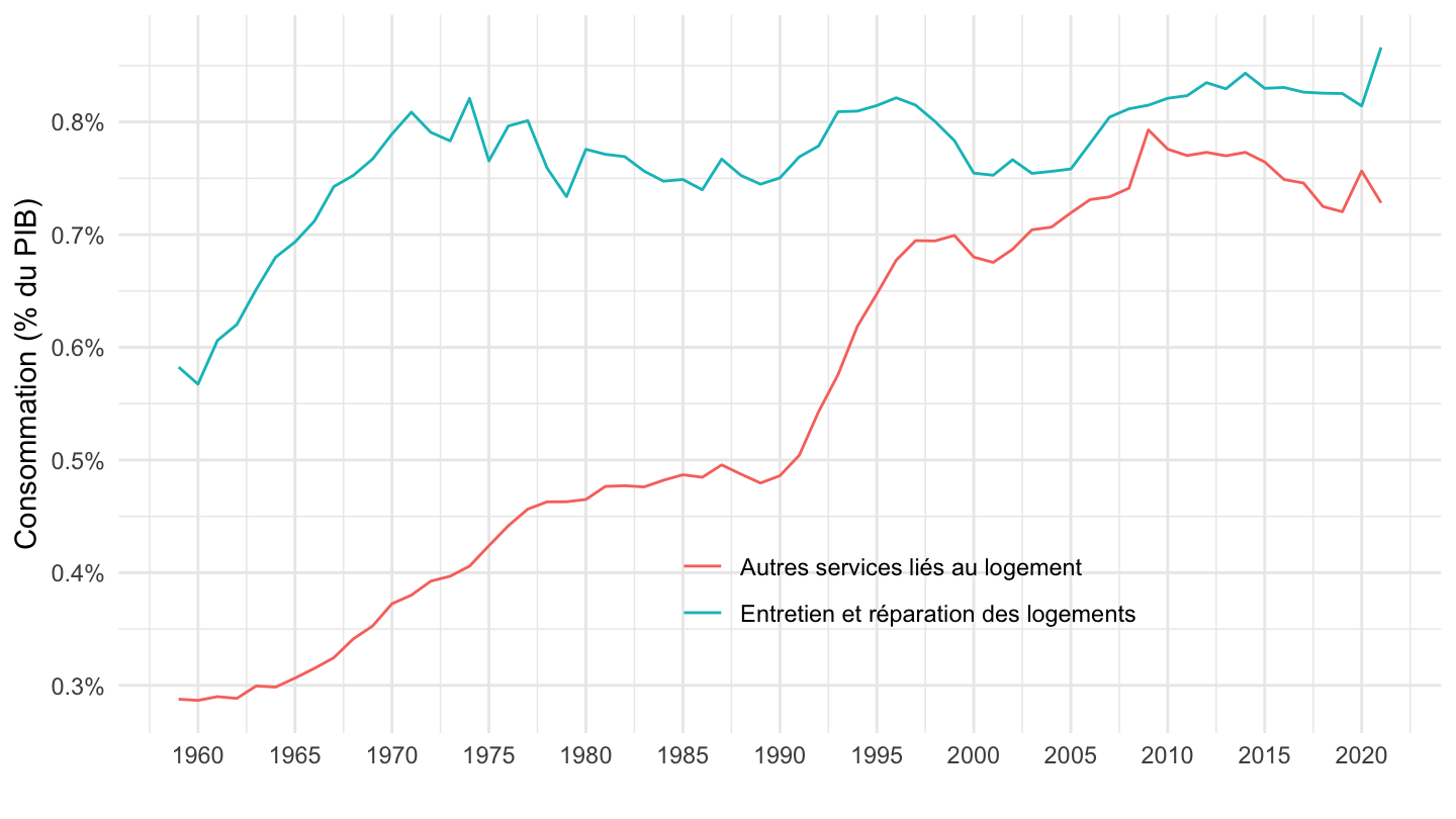
Indices de Prix
Tous
Code
`conso-eff-fonction` %>%
  filter(variable == "Iprix2014",
         year %in% c("1990", "2020")) %>%
  select(-variable) %>%
  spread(year, value) %>%
  mutate(`% / an` = round(100*((`2020`/`1990`)^(1/30)-1), 2)) %>%
  arrange(`% / an`) %>%
  print_table_conditional()
Déflateurs
Code
`conso-eff-fonction` %>%
  filter(variable == "Iprix2014") %>%
  year_to_date2 %>%
  filter(Fonction %in% c("Dépense de consommation des ménages",
                         "Dépense de consommation des ménages hors SIFIM",
                         "Consommation effective des ménages"))  %>%
  filter(date >= as.Date("1990-01-01")) %>%
  group_by(fonction) %>%
  arrange(date) %>%
  mutate(value = 100*value/value[1]) %>%
  ggplot + theme_minimal() + xlab("") + ylab("") +
  geom_line(aes(x = date, y = value, color = Fonction)) +
  scale_x_date(breaks = seq(1960, 2022, 5) %>% paste0("-01-01") %>% as.Date,
               labels = date_format("%Y")) +
  scale_y_log10(breaks = seq(100, 300, 10)) +

  theme(legend.position = c(0.25, 0.9),
        legend.title = element_blank())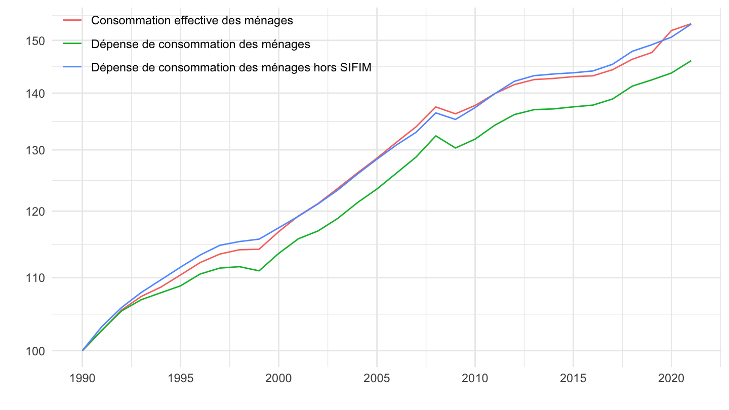
Loyers effectifs, imputés
All
Code
`conso-eff-fonction` %>%
  filter(variable == "Iprix2014") %>%
  year_to_date2 %>%
  filter(fonction %in% c("04.1", "04.2"))  %>%
  filter(date >= as.Date("1990-01-01")) %>%
  group_by(fonction) %>%
  arrange(date) %>%
  mutate(value = 100*value/value[1]) %>%
  ggplot + theme_minimal() + xlab("") + ylab("") +
  geom_line(aes(x = date, y = value, color = Fonction)) +
  scale_x_date(breaks = seq(1960, 2022, 5) %>% paste0("-01-01") %>% as.Date,
               labels = date_format("%Y")) +
  scale_y_log10(breaks = seq(100, 300, 10)) +

  theme(legend.position = c(0.25, 0.9),
        legend.title = element_blank())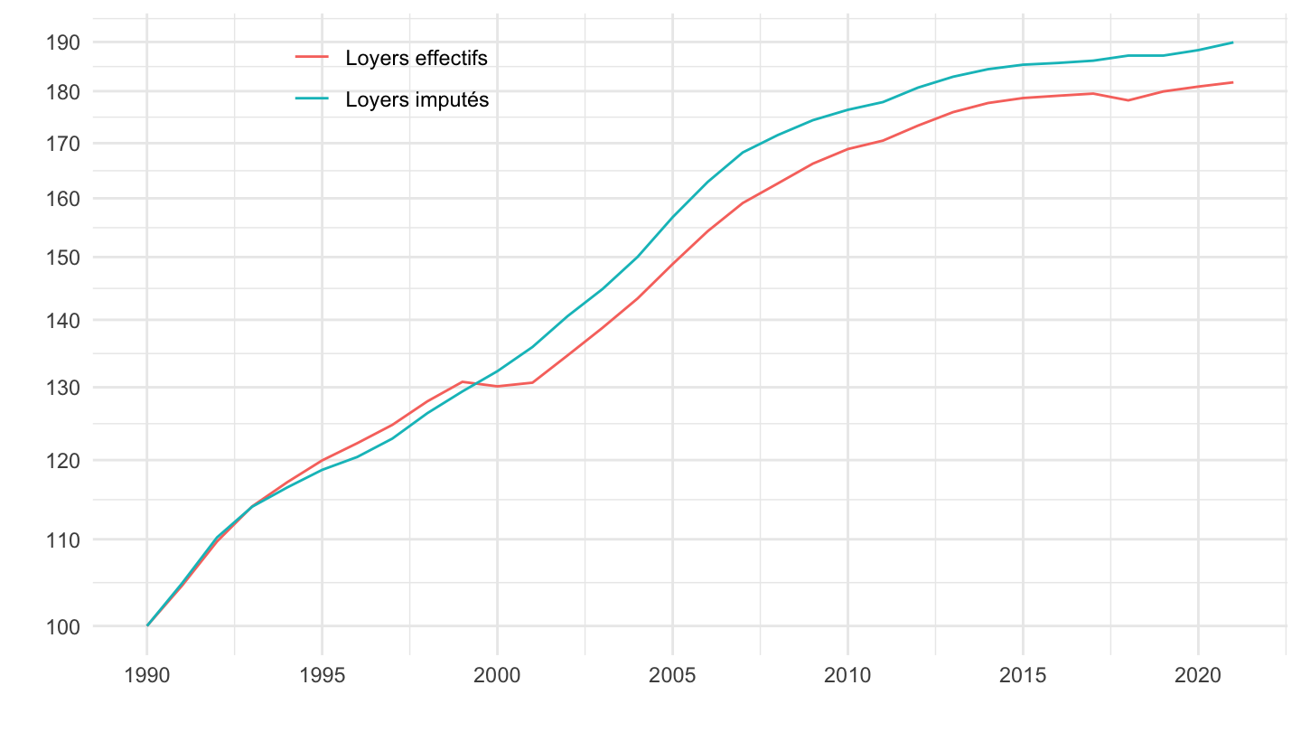
1996-
Code
`conso-eff-fonction` %>%
  filter(variable == "Iprix2014") %>%
  year_to_date2 %>%
  filter(fonction %in% c("04.1", "04.2"))  %>%
  filter(date >= as.Date("1996-01-01")) %>%
  group_by(fonction) %>%
  arrange(date) %>%
  mutate(value = 100*value/value[1]) %>%
  ggplot + theme_minimal() + xlab("") + ylab("") +
  geom_line(aes(x = date, y = value, color = Fonction)) +
  scale_x_date(breaks = seq(1996, 2022, 2) %>% paste0("-01-01") %>% as.Date,
               labels = date_format("%Y")) +
  scale_y_log10(breaks = seq(100, 300, 10)) +

  theme(legend.position = c(0.25, 0.9),
        legend.title = element_blank())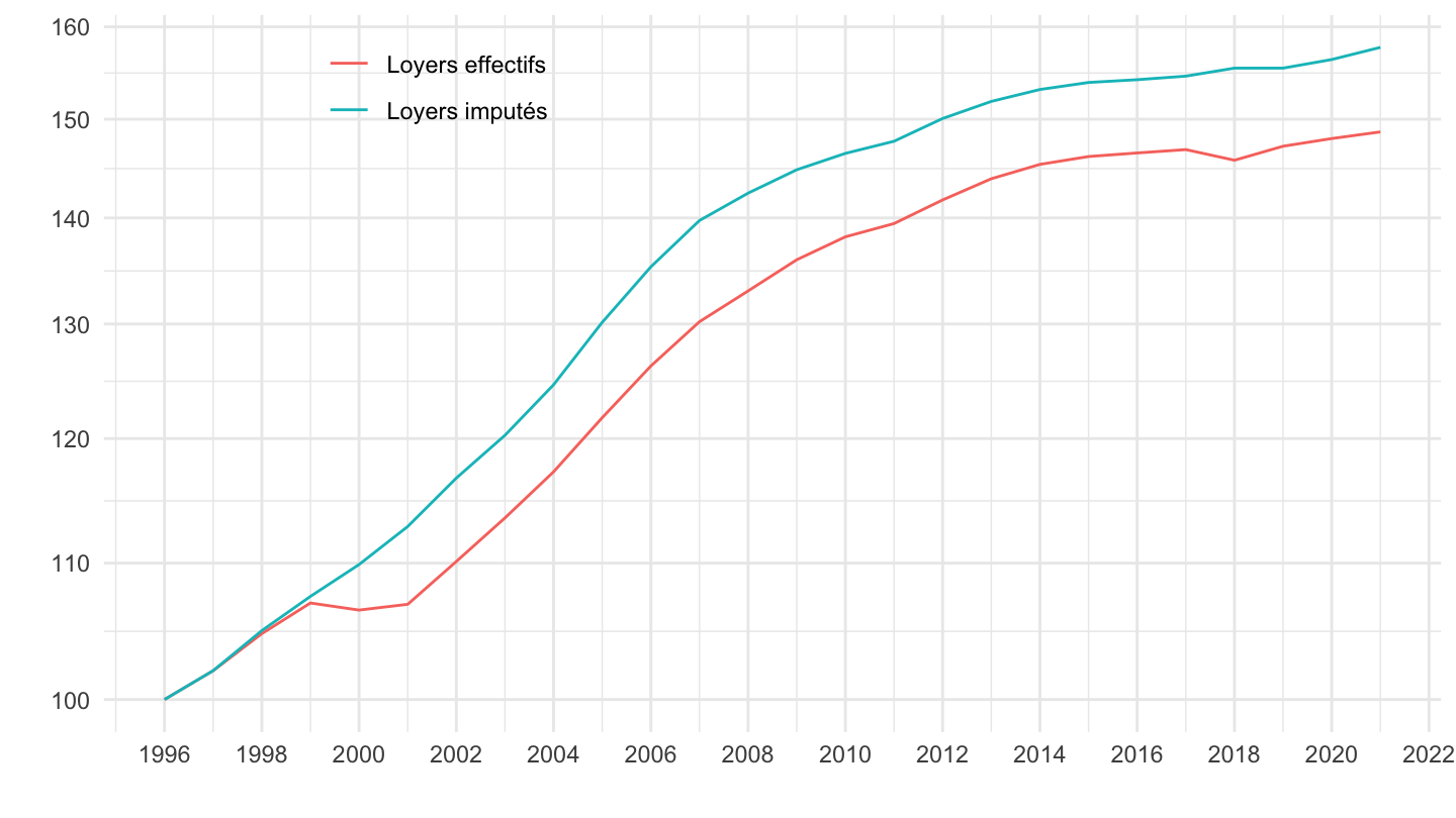
Forts effets qualité
1972-
Code
`conso-eff-fonction` %>%
  filter(variable == "Iprix2014") %>%
  year_to_date2 %>%
  filter(fonction %in% c("08.2", "09.1.3", "09.1.2", "09.1.1", "12.6.1"))  %>%
  filter(date >= as.Date("1972-01-01")) %>%
  group_by(fonction) %>%
  arrange(date) %>%
  mutate(value = 100*value/value[1]) %>%
  ggplot + theme_minimal() + xlab("") + ylab("") +
  geom_line(aes(x = date, y = value, color = Fonction)) +
  scale_x_date(breaks = seq(1960, 2022, 5) %>% paste0("-01-01") %>% as.Date,
               labels = date_format("%Y")) +
  scale_y_log10(breaks = c(0.1, 1, 2, 3, 5, 10, 20, 30, 50, 100, 200, 400, 800, 1600)) +
  theme(legend.position = c(0.35, 0.2),
        legend.title = element_blank())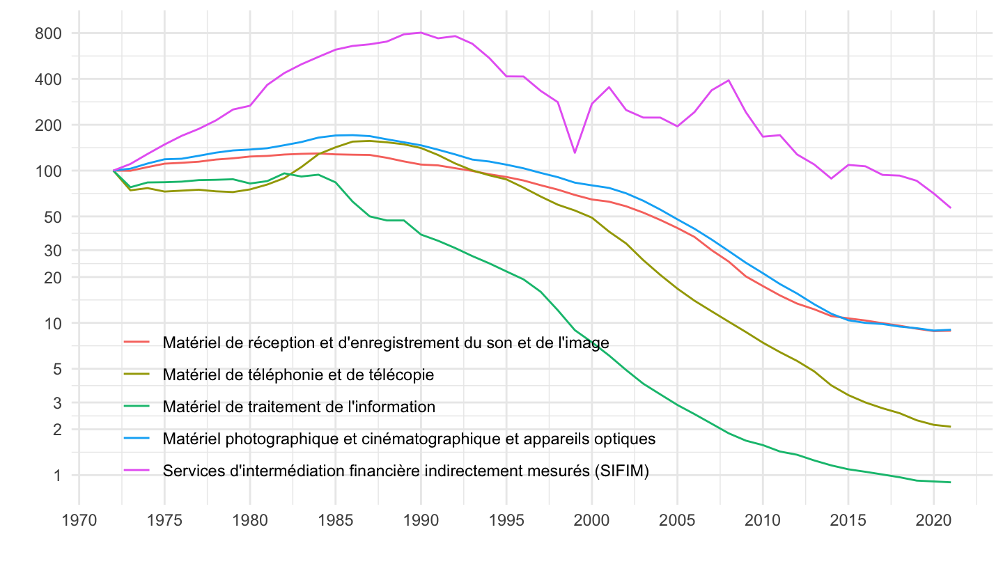
1990-
Code
`conso-eff-fonction` %>%
  filter(variable == "Iprix2014") %>%
  year_to_date2 %>%
  filter(fonction %in% c("08.2", "09.1.3", "09.1.2", "09.1.1", "12.6.1"))  %>%
  filter(date >= as.Date("1990-01-01")) %>%
  group_by(fonction) %>%
  arrange(date) %>%
  mutate(value = 100*value/value[1]) %>%
  ggplot + theme_minimal() + xlab("") + ylab("") +
  geom_line(aes(x = date, y = value, color = Fonction)) +
  scale_x_date(breaks = seq(1960, 2022, 5) %>% paste0("-01-01") %>% as.Date,
               labels = date_format("%Y")) +
  scale_y_log10(breaks = c(0.1, 1, 2, 3, 5, 10, 20, 30, 50, 100)) +
  theme(legend.position = c(0.35, 0.2),
        legend.title = element_blank())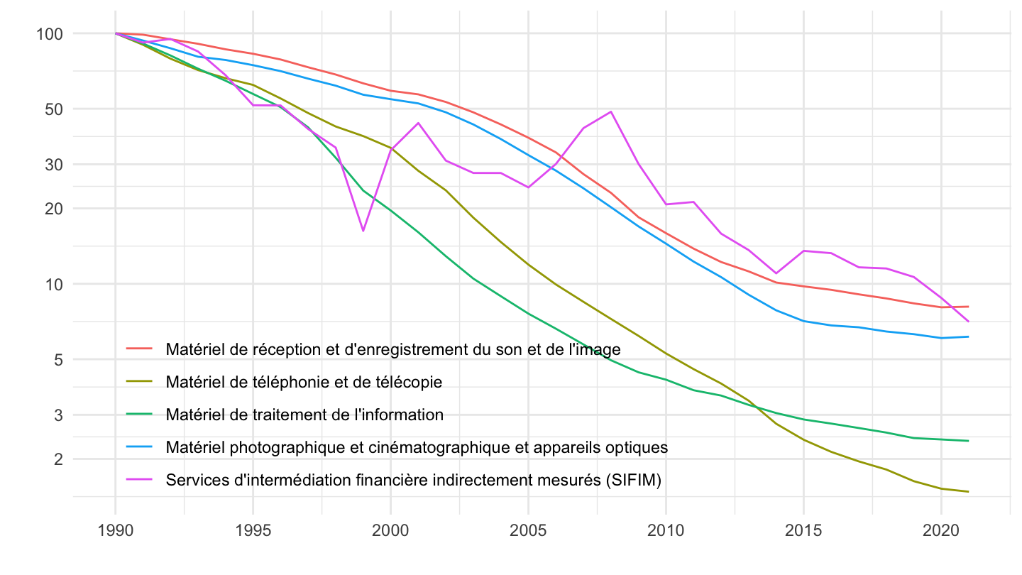
1996-
Code
`conso-eff-fonction` %>%
  filter(variable == "Iprix2014") %>%
  year_to_date2 %>%
  filter(fonction %in% c("08.2", "09.1.3", "09.1.2", "09.1.1", "12.6.1"))  %>%
  filter(date >= as.Date("1996-01-01")) %>%
  group_by(fonction) %>%
  arrange(date) %>%
  mutate(value = 100*value/value[1]) %>%
  ggplot + theme_minimal() + xlab("") + ylab("") +
  geom_line(aes(x = date, y = value, color = Fonction)) +
  scale_x_date(breaks = seq(1960, 2022, 2) %>% paste0("-01-01") %>% as.Date,
               labels = date_format("%Y")) +
  scale_y_log10(breaks = c(0.1, 1, 2, 3, 5, 10, 20, 30, 50, 100)) +
  theme(legend.position = c(0.35, 0.2),
        legend.title = element_blank())
Poids
% de la dépense de consommation finale effective
Code
`conso-eff-fonction` %>%
  filter(variable == "Coeffcour",
         year %in% c("1960", "1990", "2020")) %>%
  select(-variable) %>%
  spread(year, value) %>%
  arrange(-`2020`) %>%
  print_table_conditional()
09.1 (Matériel audiovisuel, photographique et informatique), 08.2 (Matériel de téléphonie et de télécopie)
Code
`conso-eff-fonction` %>%
  filter(variable == "Coeffcour",
         fonction %in% c("09.1", "08.2", "12.6")) %>%
  year_to_date2 %>%
  mutate(value = value / 100) %>%
  ggplot() + ylab("Pondération (% de la conso effective totale)") + xlab("") + theme_minimal() +
  geom_line(aes(x = date, y = value, color = paste0(fonction, " - ", Fonction))) +

  scale_x_date(breaks = seq(1920, 2025, 5) %>% paste0("-01-01") %>% as.Date,
               labels = date_format("%Y")) +
  theme(legend.position = c(0.28, 0.93),
        legend.title = element_blank()) +
  scale_y_continuous(breaks = 0.01*seq(0, 300, .5),
                     labels = percent_format(accuracy = .1))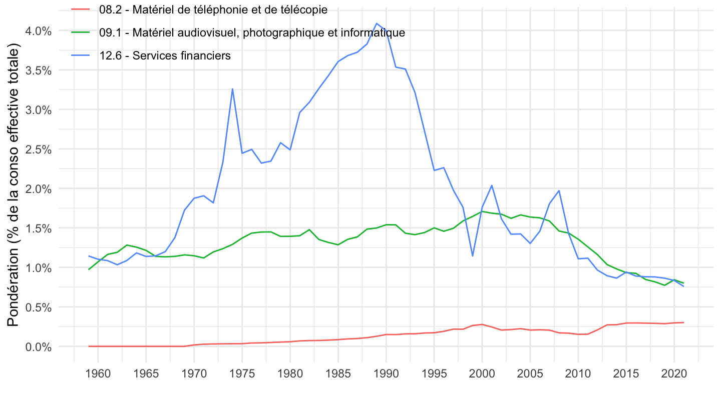
14, 01..12+15
Code
`conso-eff-fonction` %>%
  filter(variable == "Coeffcour",
         fonction %in% c("14", "01..12+15")) %>%
  year_to_date2 %>%
  mutate(value = value / 100) %>%
  ggplot() + ylab("Pondération (% de la conso effective totale)") + xlab("") + theme_minimal() +
  geom_line(aes(x = date, y = value, color = paste0(fonction, " - ", Fonction))) +

  scale_x_date(breaks = seq(1920, 2025, 5) %>% paste0("-01-01") %>% as.Date,
               labels = date_format("%Y")) +
  theme(legend.position = c(0.4, 0.6),
        legend.title = element_blank()) +
  scale_y_continuous(breaks = 0.01*seq(0, 100, 5),
                     labels = percent_format(accuracy = 1))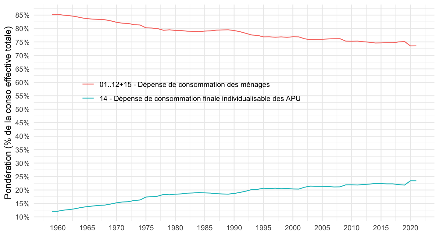
14.1, 14.2, 14.3, 14.4, 14.5
Code
`conso-eff-fonction` %>%
  filter(variable == "Coeffcour",
         fonction %in% c("14.1", "14.2", "14.3", "14.4", "14.5")) %>%
  year_to_date2 %>%
  mutate(value = value / 100) %>%
  ggplot() + ylab("Pondération (% de la conso effective totale)") + xlab("") + theme_minimal() +
  geom_line(aes(x = date, y = value, color = paste0(fonction, " - ", Fonction))) +
  #
  scale_x_date(breaks = seq(1920, 2025, 5) %>% paste0("-01-01") %>% as.Date,
               labels = date_format("%Y")) +
  theme(legend.position = c(0.2, 0.88),
        legend.title = element_blank()) +
  scale_y_continuous(breaks = 0.01*seq(0, 100, 1),
                     labels = percent_format(accuracy = 1))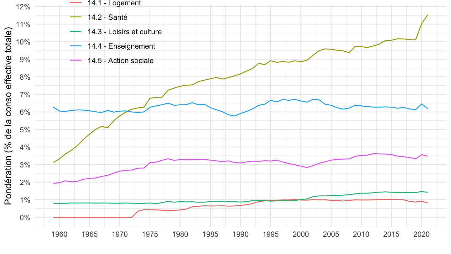
04.1, 04.2, 04.5
Code
`conso-eff-fonction` %>%
  filter(variable == "Coeffcour",
         fonction %in% c("04.1", "04.2", "04.5")) %>%
  year_to_date2 %>%
  mutate(value = value / 100) %>%
  ggplot() + ylab("Pondération (% de la conso effective totale)") + xlab("") + theme_minimal() +
  geom_line(aes(x = date, y = value, color = paste0(fonction, " - ", Fonction))) +
  #
  scale_x_date(breaks = seq(1920, 2025, 5) %>% paste0("-01-01") %>% as.Date,
               labels = date_format("%Y")) +
  theme(legend.position = c(0.28, 0.93),
        legend.title = element_blank()) +
  scale_y_continuous(breaks = 0.01*seq(0, 300, .5),
                     labels = percent_format(accuracy = .1))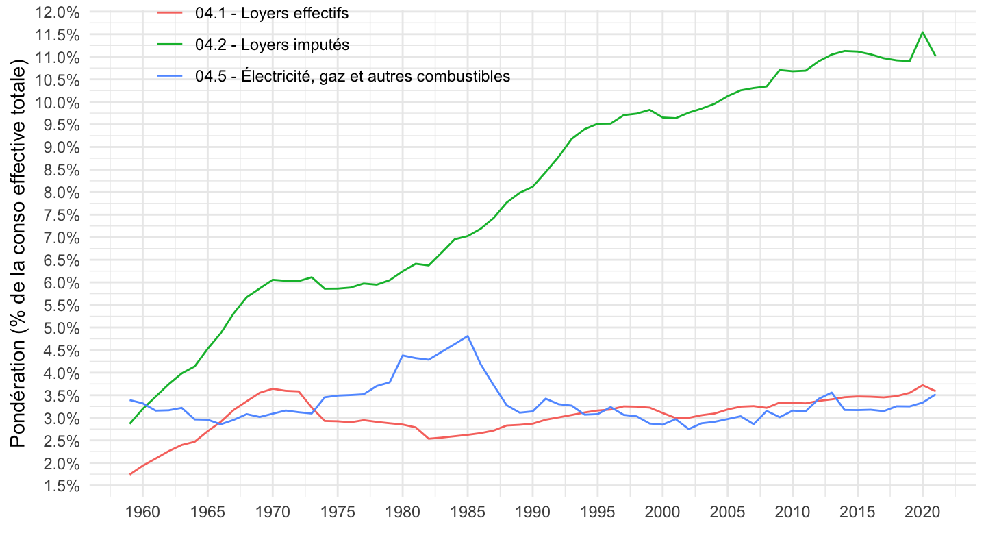
Santé
Code
`conso-eff-fonction` %>%
  filter(variable == "Coeffcour",
         fonction %in% c("14.2", "06", "12.5.3")) %>%
  year_to_date2 %>%
  mutate(value = value / 100) %>%
  ggplot() + ylab("Pondération (% de la conso effective totale)") + xlab("") + theme_minimal() +
  geom_line(aes(x = date, y = value, color = paste0(fonction, " - ", Fonction))) +

  scale_x_date(breaks = seq(1920, 2025, 5) %>% paste0("-01-01") %>% as.Date,
               labels = date_format("%Y")) +
  theme(legend.position = c(0.25, 0.93),
        legend.title = element_blank()) +
  scale_y_continuous(breaks = 0.01*seq(0, 300, .5),
                     labels = percent_format(accuracy = .1))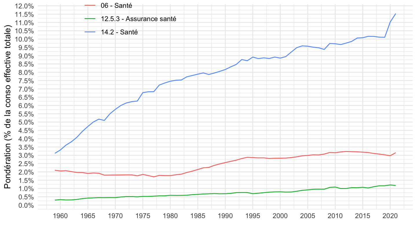
% de la dépense de consommation finale
All
Code
`conso-eff-fonction` %>%
  filter(variable == "Coeffcour",
         year %in% c("1960", "1990", "2020")) %>%
  select(-variable) %>%
  group_by(year) %>%
  arrange(fonction) %>%
  mutate(value = round(100*value/value[Fonction == "Dépense de consommation des ménages"],2)) %>%
  spread(year, value) %>%
  print_table_conditional()
2-digit
Code
`conso-eff-fonction` %>%
  filter(variable == "Coeffcour",
         year %in% c("1960", "1990", "2020"),
         nchar(fonction) == 2 | fonction == "01..12+15") %>%
  select(-variable) %>%
  group_by(year) %>%
  arrange(fonction) %>%
  mutate(value = round(100*value/value[Fonction == "Dépense de consommation des ménages"],2)) %>%
  spread(year, value) %>%
print_table_conditional()| fonction | Fonction | 1960 | 1990 | 2020 |
|---|---|---|---|---|
| 01 | Produits alimentaires et boissons non alcoolisées | 25.07 | 14.89 | 15.02 |
| 01..12+15 | Dépense de consommation des ménages | 100.00 | 100.00 | 100.00 |
| 02 | Boissons alcoolisées et tabac | 7.13 | 3.42 | 4.39 |
| 03 | Articles d'habillement et chaussures | 11.95 | 6.79 | 3.14 |
| 04 | Logement, eau, gaz, électricité et autres combustibles | 11.45 | 20.13 | 28.38 |
| 05 | Meubles, articles de ménage et entretien courant de l'habitation | 8.54 | 6.19 | 4.88 |
| 06 | Santé | 2.41 | 3.23 | 4.05 |
| 07 | Transports | 10.58 | 15.09 | 11.77 |
| 08 | Communications | 0.60 | 2.10 | 2.56 |
| 09 | Loisirs et culture | 7.09 | 8.58 | 7.58 |
| 10 | Éducation | 0.31 | 0.35 | 0.49 |
| 11 | Hôtels, cafés et restaurants | 6.67 | 6.17 | 5.53 |
| 12 | Biens et services divers | 7.41 | 13.74 | 12.80 |
| 13 | Dépense de consommation finale individualisable des ISBLSM | 3.08 | 2.59 | 4.15 |
| 14 | Dépense de consommation finale individualisable des APU | 14.21 | 23.59 | 31.87 |
| 15 | Solde territorial | 0.78 | -0.67 | -0.59 |
3-digit
Code
`conso-eff-fonction` %>%
  filter(variable == "Coeffcour",
         year %in% c("1960", "1990", "2020"),
         nchar(fonction) == 4 | fonction == "01..12+15") %>%
  select(-variable) %>%
  group_by(year) %>%
  arrange(fonction) %>%
  mutate(value = round(100*value/value[Fonction == "Dépense de consommation des ménages"],2)) %>%
  spread(year, value) %>%
  print_table_conditional()
4-digit
Code
`conso-eff-fonction` %>%
  filter(variable == "Coeffcour",
         year %in% c("1960", "1990", "2020"),
         nchar(fonction) == 6 | fonction == "01..12+15") %>%
  select(-variable) %>%
  group_by(year) %>%
  arrange(fonction) %>%
  mutate(value = round(100*value/value[Fonction == "Dépense de consommation des ménages"],2)) %>%
  spread(year, value) %>%
  print_table_conditional()
Comparer IPC, IPCH, Déflateur de la consommation
Table Déflateur
Code
deflateur <- `conso-eff-fonction` %>%
  filter(variable == "Iprix2014",
         year %in% c("1990", "2020"),
         nchar(fonction) %in% c(2, 4, 6)) %>%
  mutate(fonction = gsub("\\.", "", fonction)) %>%
  select(fonction, Fonction, year, value) %>%
  spread(year, value) %>%
  mutate(`Déflateur (%)` = round(100*((`2020`/`1990`)^(1/30)-1),2)) %>%
  select(-`1990`, -`2020`)

deflateur %>%
  print_table_conditional
Table Déflateur Poids
Code
deflateur_poids <- `conso-eff-fonction` %>%
  filter(variable == "Coeffcour",
         year %in% c("2020"),
         nchar(fonction) %in% c(2, 4, 6)) %>%
  mutate(fonction = gsub("\\.", "", fonction)) %>%
  select(fonction, Fonction, year, value) %>%
  spread(year, value) %>%
  rename(`Déflateur Poids` = `2020`)

deflateur_poids %>%
  print_table_conditional
Table IPC
Code
IPC <- `IPC-2015` %>%
  filter(INDICATEUR == "IPC",
         MENAGES_IPC == "ENSEMBLE",
         FREQ == "M",
         REF_AREA == "FE",
         NATURE == "INDICE",
         TIME_PERIOD %in% c("1990-01", "2020-01")) %>%
  left_join(COICOP2016, by = "COICOP2016") %>%
  select(fonction = COICOP2016, Fonction = Coicop2016, TIME_PERIOD, OBS_VALUE) %>%
  filter(!(fonction %in% c("SO", "00"))) %>%
  spread(TIME_PERIOD, OBS_VALUE) %>%
  mutate(`IPC (%)` = round(100*((`2020-01`/`1990-01`)^(1/30)-1),2)) %>%
  select(-`1990-01`, -`2020-01`)

IPC %>%
  print_table_conditional()
Table IPC Poids
Code
IPC_poids <- `IPC-2015` %>%
  filter(INDICATEUR == "IPC",
         REF_AREA == "FE",
         MENAGES_IPC == "ENSEMBLE",
         NATURE == "POND",
         TIME_PERIOD %in% c("2020")) %>%
  left_join(COICOP2016, by = "COICOP2016") %>%
  select(fonction = COICOP2016, Fonction = Coicop2016, TIME_PERIOD, OBS_VALUE) %>%
  filter(!(fonction %in% c("SO", "00"))) %>%
  mutate(OBS_VALUE = OBS_VALUE/100) %>%
  spread(TIME_PERIOD, OBS_VALUE) %>%
  rename(`IPC Poids` = `2020`)

IPC_poids %>%
  print_table_conditional()
Comparer Table Déflateur VS IPC
Tous
Code
deflateur %>%
  inner_join(IPC, by = "fonction") %>%
  mutate(Difference = `Déflateur (%)`-`IPC (%)`) %>%
  arrange(Difference) %>%
  print_table_conditional()
2-digit
Code
deflateur %>%
  inner_join(IPC, by = "fonction") %>%
  filter(nchar(fonction) == 2) %>%
  mutate(Difference = `Déflateur (%)`-`IPC (%)`) %>%
  arrange(Difference) %>%
print_table_conditional()| fonction | Fonction.x | Déflateur (%) | Fonction.y | IPC (%) | Difference |
|---|---|---|---|---|---|
| 08 | Communications | -4.30 | 08 - Communications | -1.80 | -2.50 |
| 12 | Biens et services divers | 0.48 | 12 - Biens et services divers | 1.91 | -1.43 |
| 09 | Loisirs et culture | -0.63 | 09 - Loisirs et culture | 0.05 | -0.68 |
| 05 | Meubles, articles de ménage et entretien courant de l'habitation | 0.62 | 05 - Meubles, articles de ménage et entretien courant du foyer | 1.02 | -0.40 |
| 07 | Transports | 1.75 | 07 - Transports | 2.14 | -0.39 |
| 02 | Boissons alcoolisées et tabac | 3.99 | 02 - Boissons alcoolisées, tabac et stupéfiants | 4.33 | -0.34 |
| 04 | Logement, eau, gaz, électricité et autres combustibles | 2.20 | 04 - Logement, eau, gaz, électricité et autres combustibles | 2.36 | -0.16 |
| 11 | Hôtels, cafés et restaurants | 2.34 | 11 - Restaurants et hôtels | 2.47 | -0.13 |
| 10 | Éducation | 2.16 | 10 - Enseignement | 2.28 | -0.12 |
| 01 | Produits alimentaires et boissons non alcoolisées | 1.49 | 01 - Produits alimentaires et boissons non alcoolisées | 1.52 | -0.03 |
| 03 | Articles d'habillement et chaussures | 0.54 | 03 - Articles d'habillement et chaussures | 0.33 | 0.21 |
| 06 | Santé | 0.40 | 06 - Santé | 0.19 | 0.21 |
3-digit
Code
deflateur %>%
  inner_join(IPC, by = "fonction") %>%
  filter(nchar(fonction) == 3) %>%
  mutate(Difference = `Déflateur (%)`-`IPC (%)`) %>%
  arrange(Difference) %>%
  print_table_conditional()
4-digit
Code
deflateur %>%
  inner_join(IPC, by = "fonction") %>%
  filter(nchar(fonction) == 4) %>%
  mutate(Difference = `Déflateur (%)`-`IPC (%)`) %>%
  arrange(Difference) %>%
  print_table_conditional()
Comparer Poids Déflateur VS IPC
Code
deflateur_poids %>%
  inner_join(IPC_poids, by = "fonction") %>%
  mutate(Difference = `Déflateur Poids`-`IPC Poids`) %>%
  arrange(Difference) %>%
  print_table_conditional()
2-digit
00 - Tous
1996-
Code
`conso-eff-fonction` %>%
  filter(Fonction %in% c("Consommation effective des ménages",
                         "Dépense de consommation des ménages",
                         "Dépense de consommation des ménages hors SIFIM"),
         variable == "Iprix2014") %>%
  mutate(Fonction = ifelse(Fonction == "Consommation effective des ménages",
                           "Dépense de consommation effective des ménages",
                           Fonction)) %>%
  year_to_date2 %>%
  filter(date >= as.Date("1996-01-01")) %>%
  select(variable = Fonction, date, value) %>%
  mutate(variable = paste0("Déflateur de la ", variable)) %>%
  bind_rows(`IPC-2015` %>%
              filter(INDICATEUR == "IPC",
                     MENAGES_IPC == "ENSEMBLE",
                     COICOP2016 %in% c("00"),
                     FREQ == "M",
                     PRIX_CONSO == "SO",
                     REF_AREA == "FE",
                     NATURE == "INDICE") %>%
              month_to_date %>%
              filter(month(date) == 1) %>%
              mutate(variable = "Indice des Prix à la Consommation (IPC)") %>%
              select(variable, date, value = OBS_VALUE)) %>%
  bind_rows(`IPCH-2015` %>%
              filter(INDICATEUR == "IPCH",
                     COICOP2016 %in% c("00"),
                     FREQ == "M",
                     REF_AREA == "FE",
                     NATURE == "INDICE") %>%
              month_to_date %>%
              filter(month(date) == 1) %>%
              mutate(variable = "Indice des Prix à la Consommation Harmonisé (IPCH)") %>%
              select(variable, date, value = OBS_VALUE)) %>%
  group_by(variable) %>%
  filter(date >= as.Date("1996-01-01")) %>%
  mutate(value = 100*value/value[date == as.Date("1996-01-01")]) %>%
  mutate(variable = gsub("Indice des prix à la consommation - Base 2015 - Ensemble des ménages - France - ", "", variable)) %>%
  ggplot() + ylab("Indice des prix") + xlab("") + theme_minimal() +
  geom_line(aes(x = date, y = value, color = variable)) +
  #
  scale_x_date(breaks = seq(1920, 2025, 2) %>% paste0("-01-01") %>% as.Date,
               labels = date_format("%Y")) +
  theme(legend.position = c(0.3, 0.8),
        legend.title = element_blank()) +
  scale_y_log10(breaks = seq(0, 500, 10),
                     labels = dollar_format(accuracy = 1, prefix = ""))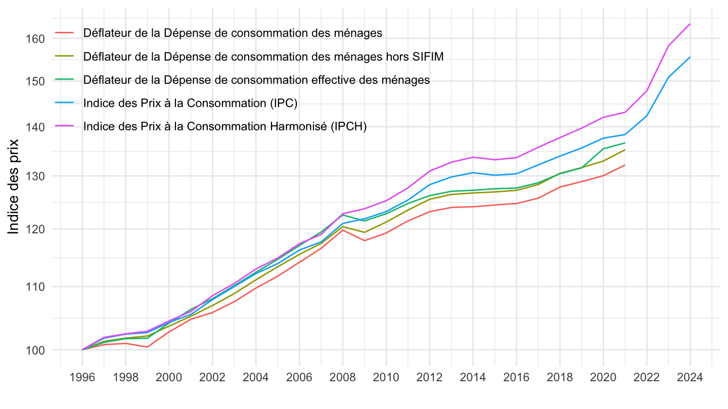
2000-
Code
`conso-eff-fonction` %>%
  filter(Fonction %in% c("Consommation effective des ménages",
                         "Dépense de consommation des ménages",
                         "Dépense de consommation des ménages hors SIFIM"),
         variable == "Iprix2014") %>%
  mutate(Fonction = ifelse(Fonction == "Consommation effective des ménages",
                           "Dépense de consommation effective des ménages",
                           Fonction)) %>%
  year_to_date2 %>%
  filter(date >= as.Date("2000-01-01")) %>%
  select(variable = Fonction, date, value) %>%
  mutate(variable = paste0("Déflateur de la ", variable)) %>%
  bind_rows(`IPC-2015` %>%
              filter(INDICATEUR == "IPC",
                     MENAGES_IPC == "ENSEMBLE",
                     COICOP2016 %in% c("00"),
                     FREQ == "M",
                     PRIX_CONSO == "SO",
                     REF_AREA == "FE",
                     NATURE == "INDICE") %>%
              month_to_date %>%
              filter(month(date) == 1) %>%
              mutate(variable = "Indice des Prix à la Consommation (IPC)") %>%
              select(variable, date, value = OBS_VALUE)) %>%
  bind_rows(`IPCH-2015` %>%
              filter(INDICATEUR == "IPCH",
                     COICOP2016 %in% c("00"),
                     FREQ == "M",
                     REF_AREA == "FE",
                     NATURE == "INDICE") %>%
              month_to_date %>%
              filter(month(date) == 1) %>%
              mutate(variable = "Indice des Prix à la Consommation Harmonisé (IPCH)") %>%
              select(variable, date, value = OBS_VALUE)) %>%
  group_by(variable) %>%
  filter(date >= as.Date("2000-01-01")) %>%
  mutate(value = 100*value/value[date == as.Date("2000-01-01")]) %>%
  mutate(variable = gsub("Indice des prix à la consommation - Base 2015 - Ensemble des ménages - France - ", "", variable)) %>%
  ggplot() + ylab("Indice des prix") + xlab("") + theme_minimal() +
  geom_line(aes(x = date, y = value, color = variable)) +
  #
  scale_x_date(breaks = seq(1920, 2025, 2) %>% paste0("-01-01") %>% as.Date,
               labels = date_format("%Y")) +
  theme(legend.position = c(0.3, 0.8),
        legend.title = element_blank()) +
  scale_y_log10(breaks = seq(0, 500, 10),
                     labels = dollar_format(accuracy = 1, prefix = ""))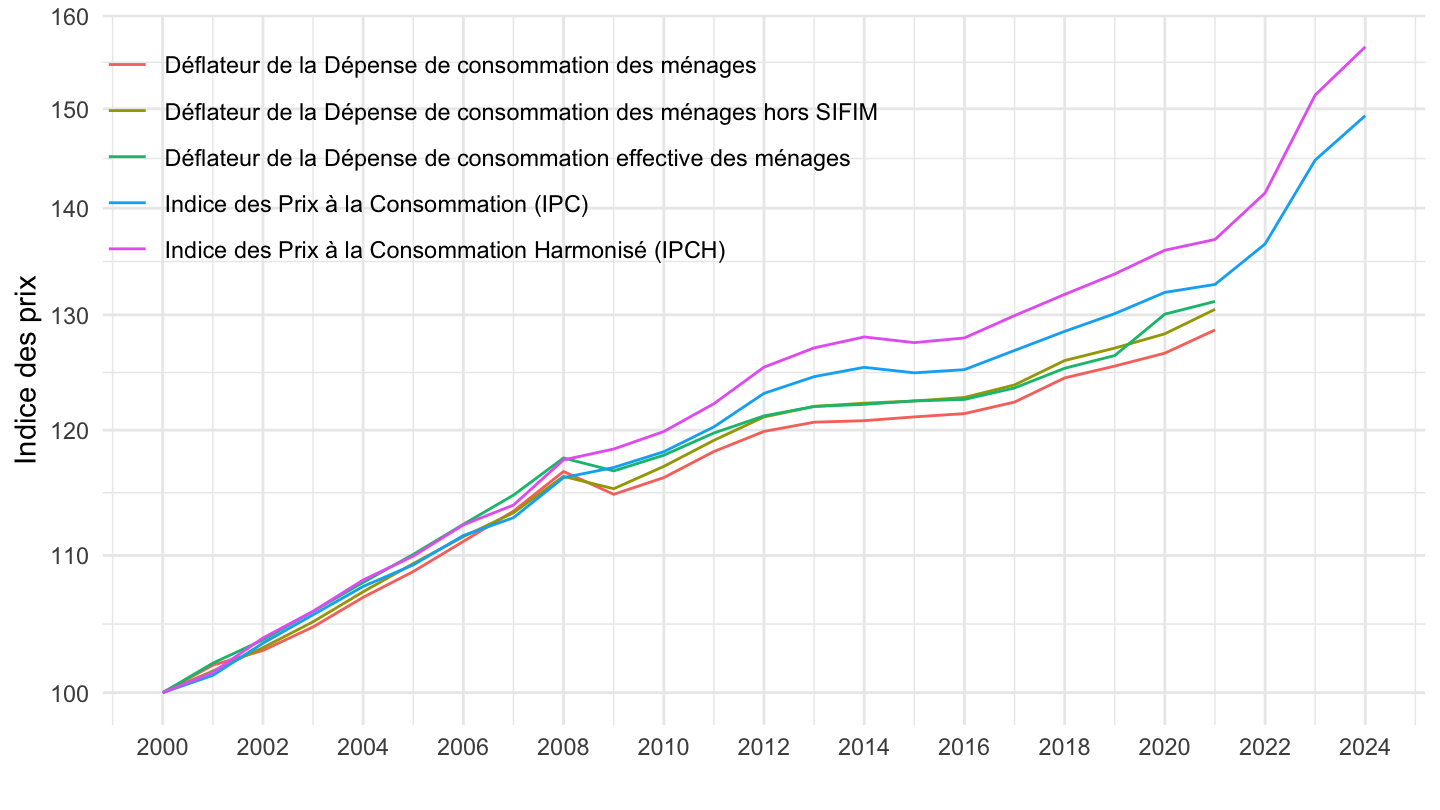
2017-
Code
`conso-eff-fonction` %>%
  filter(Fonction %in% c("Consommation effective des ménages",
                         "Dépense de consommation des ménages",
                         "Dépense de consommation des ménages hors SIFIM"),
         variable == "Iprix2014") %>%
  mutate(Fonction = ifelse(Fonction == "Consommation effective des ménages",
                           "Dépense de consommation effective des ménages",
                           Fonction)) %>%
  year_to_date2 %>%
  filter(date >= as.Date("2017-01-01")) %>%
  select(variable = Fonction, date, value) %>%
  mutate(variable = paste0("Déflateur de la ", variable)) %>%
  bind_rows(`IPC-2015` %>%
              filter(INDICATEUR == "IPC",
                     MENAGES_IPC == "ENSEMBLE",
                     COICOP2016 %in% c("00"),
                     FREQ == "M",
                     PRIX_CONSO == "SO",
                     REF_AREA == "FE",
                     NATURE == "INDICE") %>%
              month_to_date %>%
              filter(month(date) == 1) %>%
              mutate(variable = "Indice des Prix à la Consommation (IPC)") %>%
              select(variable, date, value = OBS_VALUE)) %>%
  bind_rows(`IPCH-2015` %>%
              filter(INDICATEUR == "IPCH",
                     COICOP2016 %in% c("00"),
                     FREQ == "M",
                     REF_AREA == "FE",
                     NATURE == "INDICE") %>%
              month_to_date %>%
              filter(month(date) == 1) %>%
              mutate(variable = "Indice des Prix à la Consommation Harmonisé (IPCH)") %>%
              select(variable, date, value = OBS_VALUE)) %>%
  group_by(variable) %>%
  filter(date >= as.Date("2017-01-01")) %>%
  mutate(value = 100*value/value[date == as.Date("2017-01-01")]) %>%
  mutate(variable = gsub("Indice des prix à la consommation - Base 2015 - Ensemble des ménages - France - ", "", variable)) %>%
  ggplot() + ylab("Indice des prix") + xlab("") + theme_minimal() +
  geom_line(aes(x = date, y = value, color = variable)) +
  #
  scale_x_date(breaks = seq(1920, 2025, 1) %>% paste0("-01-01") %>% as.Date,
               labels = date_format("%Y")) +
  theme(legend.position = c(0.35, 0.8),
        legend.title = element_blank()) +
  scale_y_log10(breaks = seq(0, 500, 1),
                     labels = dollar_format(accuracy = 1, prefix = ""))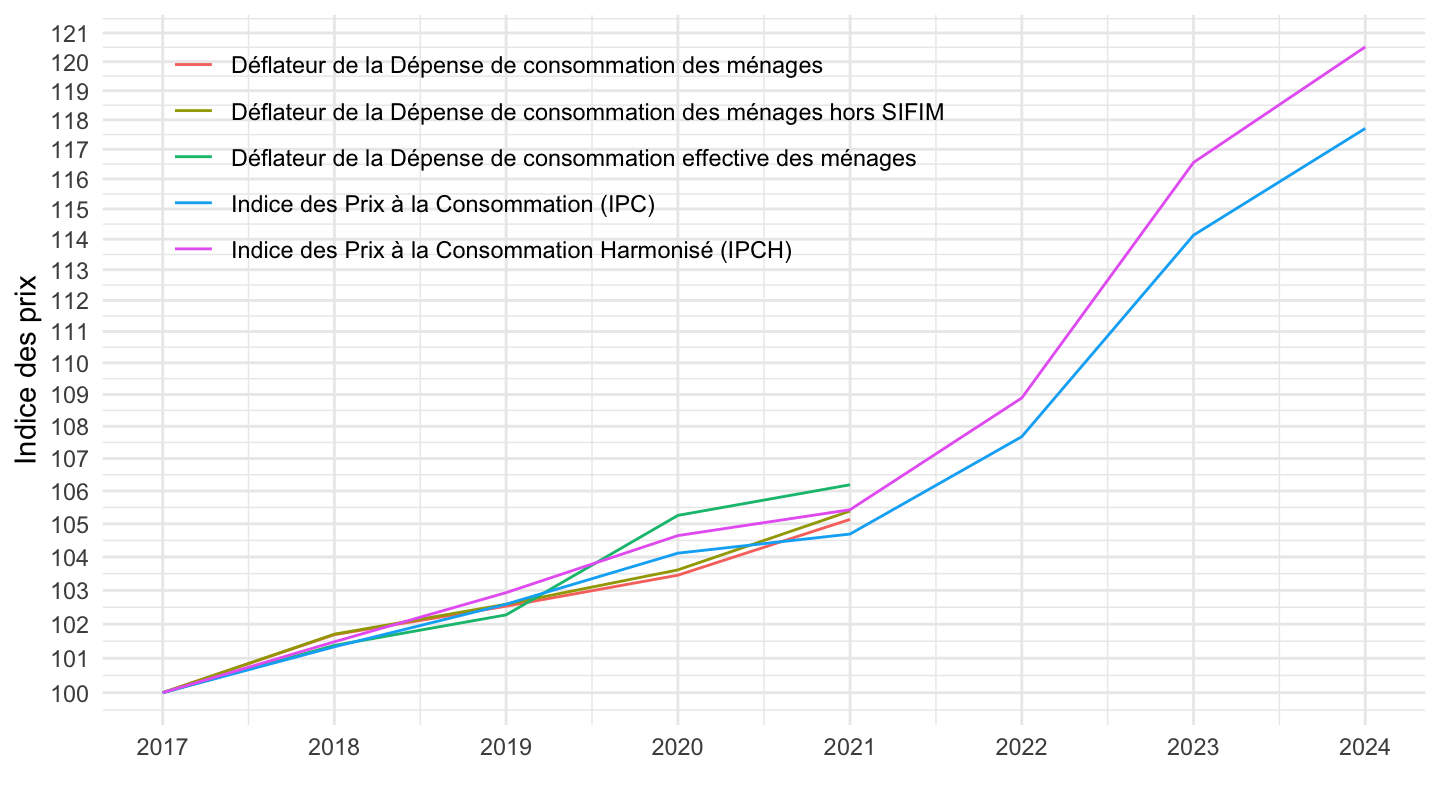
00 - Tous
All
2000-
Code
`conso-eff-fonction` %>%
  filter(Fonction %in% c("Consommation effective des ménages",
                         "Dépense de consommation des ménages",
                         "Dépense de consommation des ménages hors SIFIM"),
         variable == "Iprix2014") %>%
  year_to_date2 %>%
  filter(date >= as.Date("1990-01-01")) %>%
  select(variable = Fonction, date, value) %>%
  bind_rows(`IPC-2015` %>%
              filter(INDICATEUR == "IPC",
                     MENAGES_IPC == "ENSEMBLE",
                     COICOP2016 %in% c("00"),
                     FREQ == "M",
                     REF_AREA == "FE",
                     NATURE == "INDICE") %>%
              month_to_date %>%
  filter(month(date) == 1) %>%
  select(variable = TITLE_FR, date, value = OBS_VALUE)
  ) %>%
  group_by(variable) %>%
  mutate(value = 100*value/value[date == as.Date("1990-01-01")]) %>%
  mutate(variable = gsub("Indice des prix à la consommation - Base 2015 - Ensemble des ménages - France - ", "", variable)) %>%
  ggplot() + ylab("Indice des prix") + xlab("") + theme_minimal() +
  geom_line(aes(x = date, y = value, color = variable)) +
  #
  scale_x_date(breaks = seq(1920, 2025, 5) %>% paste0("-01-01") %>% as.Date,
               labels = date_format("%Y")) +
  theme(legend.position = c(0.25, 0.8),
        legend.title = element_blank()) +
  scale_y_log10(breaks = seq(0, 500, 10),
                     labels = dollar_format(accuracy = 1, prefix = ""))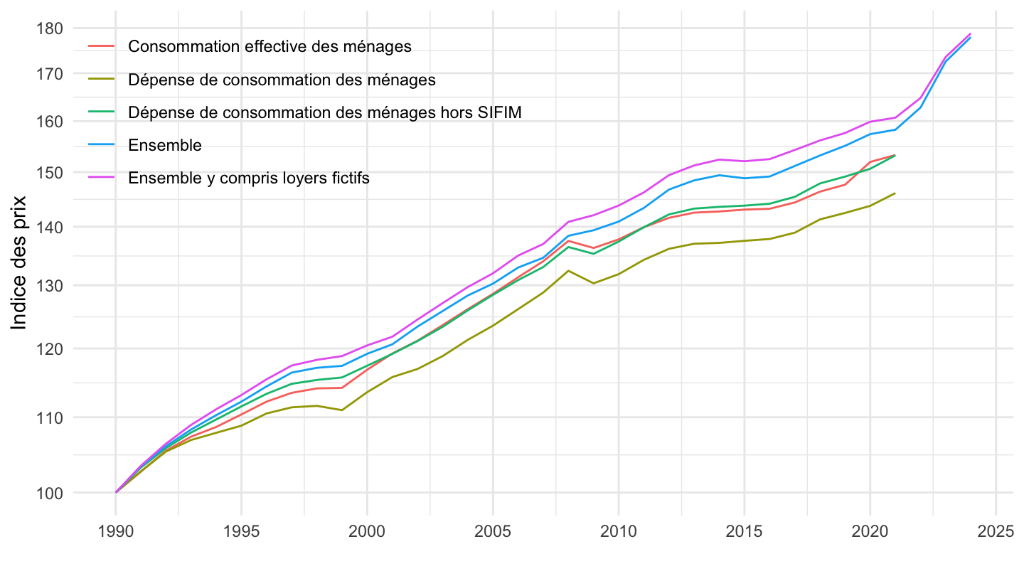
1996-
Code
`conso-eff-fonction` %>%
  filter(Fonction %in% c("Consommation effective des ménages",
                         "Dépense de consommation des ménages",
                         "Dépense de consommation des ménages hors SIFIM"),
         variable == "Iprix2014") %>%
  year_to_date2 %>%
  filter(date >= as.Date("1996-01-01")) %>%
  select(variable = Fonction, date, value) %>%
  bind_rows(`IPC-2015` %>%
              filter(INDICATEUR == "IPC",
                     MENAGES_IPC == "ENSEMBLE",
                     COICOP2016 %in% c("00"),
                     FREQ == "M",
                     REF_AREA == "FE",
                     NATURE == "INDICE") %>%
              month_to_date %>%
              filter(month(date) == 1,
                     date >= as.Date("1996-01-01")) %>%
              select(variable = TITLE_FR, date, value = OBS_VALUE)
            ) %>%
  group_by(variable) %>%
  mutate(value = 100*value/value[date == as.Date("1996-01-01")]) %>%
  mutate(variable = gsub("Indice des prix à la consommation - Base 2015 - Ensemble des ménages - France - ", "", variable)) %>%
  ggplot() + ylab("Indice des prix") + xlab("") + theme_minimal() +
  geom_line(aes(x = date, y = value, color = variable)) +
  #
  scale_x_date(breaks = seq(1920, 2025, 2) %>% paste0("-01-01") %>% as.Date,
               labels = date_format("%Y")) +
  theme(legend.position = c(0.25, 0.8),
        legend.title = element_blank()) +
  scale_y_log10(breaks = seq(0, 500, 10),
                     labels = dollar_format(accuracy = 1, prefix = ""))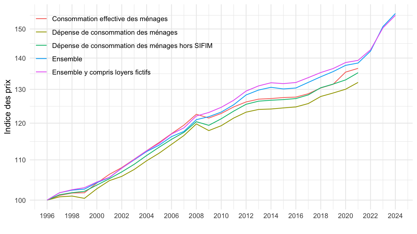
01 - Produits alimentaires et boissons non alcoolisées
Code
`conso-eff-fonction` %>%
  filter(fonction == "01",
         variable == "Iprix2014") %>%
  year_to_date2 %>%
  filter(date >= as.Date("1990-01-01")) %>%
  mutate(variable = "Deflateur de la Consommation") %>%
  select(variable, date, value) %>%
  bind_rows(`IPC-2015` %>%
              filter(INDICATEUR == "IPC",
                     MENAGES_IPC == "ENSEMBLE",
         COICOP2016 %in% c("01"),
         FREQ == "M",
         REF_AREA == "FE",
         NATURE == "INDICE") %>%
  month_to_date %>%
  filter(month(date) == 1) %>%
  select(date, value = OBS_VALUE) %>%
  mutate(variable = "Indice des Prix à la Consommation")) %>%
  group_by(variable) %>%
  mutate(value = 100*value/value[date == as.Date("1990-01-01")]) %>%
  ggplot() + ylab("Indice des prix") + xlab("") + theme_minimal() +
  geom_line(aes(x = date, y = value, color = variable)) +

  scale_x_date(breaks = seq(1920, 2025, 5) %>% paste0("-01-01") %>% as.Date,
               labels = date_format("%Y")) +
  theme(legend.position = c(0.75, 0.3),
        legend.title = element_blank()) +
  scale_y_log10(breaks = seq(0, 500, 10),
                     labels = dollar_format(accuracy = 1, prefix = ""))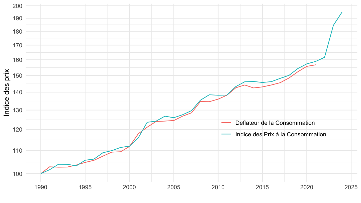
02 - Boissons alcoolisées et tabac
Code
`conso-eff-fonction` %>%
  filter(fonction == "02",
         variable == "Iprix2014") %>%
  year_to_date2 %>%
  filter(date >= as.Date("1990-01-01")) %>%
  mutate(variable = "Deflateur de la Consommation") %>%
  select(variable, date, value) %>%
  bind_rows(`IPC-2015` %>%
              filter(INDICATEUR == "IPC",
                     MENAGES_IPC == "ENSEMBLE",
                     COICOP2016 %in% c("02"),
                     FREQ == "M",
                     REF_AREA == "FE",
                     NATURE == "INDICE") %>%
              month_to_date %>%
              filter(month(date) == 1) %>%
              select(date, value = OBS_VALUE) %>%
              mutate(variable = "Indice des Prix à la Consommation")) %>%
  group_by(variable) %>%
  mutate(value = 100*value/value[date == as.Date("1990-01-01")]) %>%
  ggplot() + ylab("Indice des prix") + xlab("") + theme_minimal() +
  geom_line(aes(x = date, y = value, color = variable)) +

  scale_x_date(breaks = seq(1920, 2025, 5) %>% paste0("-01-01") %>% as.Date,
               labels = date_format("%Y")) +
  theme(legend.position = c(0.75, 0.3),
        legend.title = element_blank()) +
  scale_y_log10(breaks = seq(0, 500, 10),
                     labels = dollar_format(accuracy = 1, prefix = ""))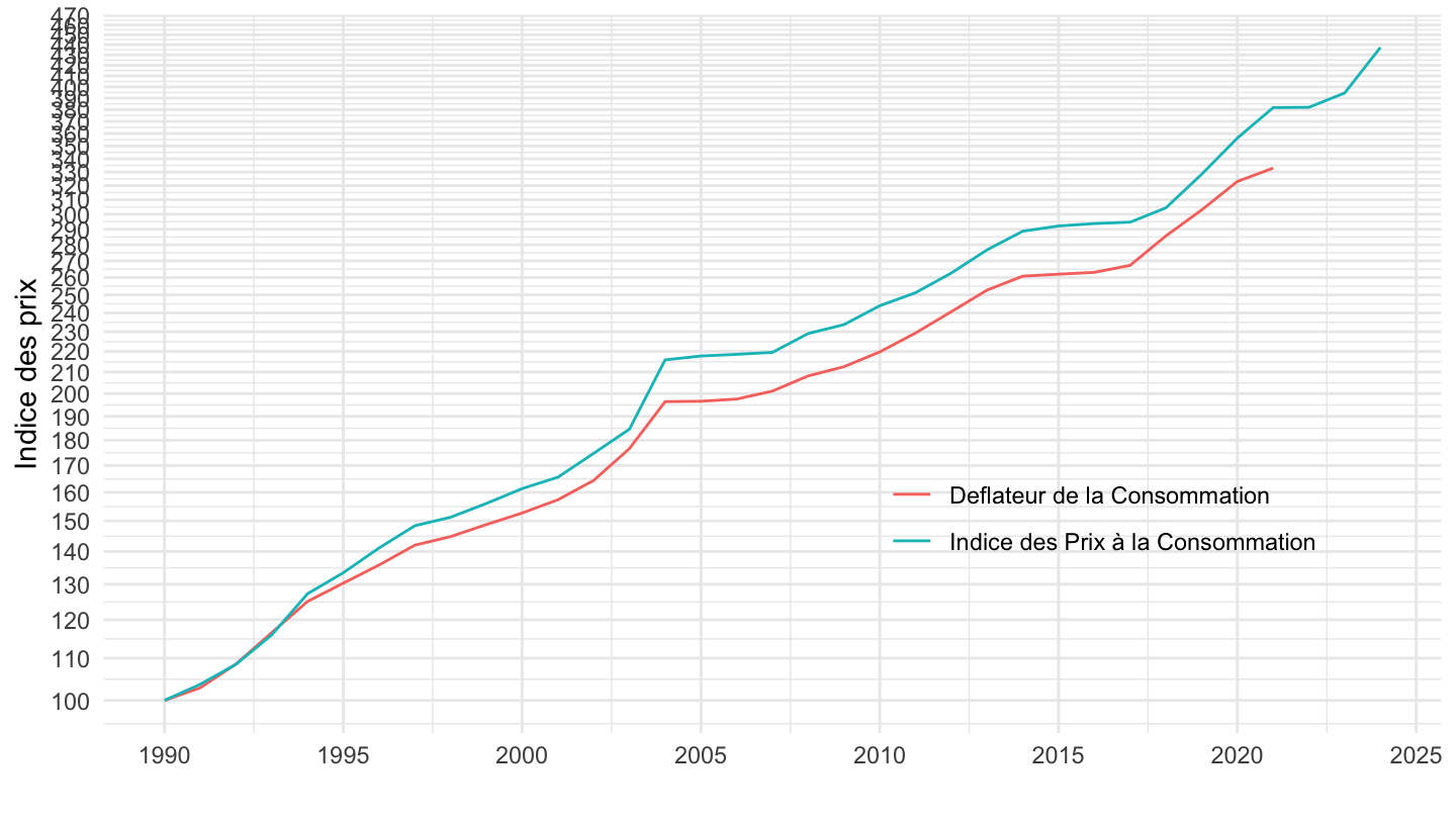
03 - Articles d’habillement et chaussures
Code
`conso-eff-fonction` %>%
  filter(fonction == "03",
         variable == "Iprix2014") %>%
  year_to_date2 %>%
  filter(date >= as.Date("1990-01-01")) %>%
  mutate(variable = "Deflateur de la Consommation") %>%
  select(variable, date, value) %>%
  bind_rows(`IPC-2015` %>%
              filter(INDICATEUR == "IPC",
                     MENAGES_IPC == "ENSEMBLE",
                     COICOP2016 %in% c("03"),
                     FREQ == "M",
                     REF_AREA == "FE",
                     NATURE == "INDICE") %>%
              month_to_date %>%
              filter(month(date) == 1) %>%
              select(date, value = OBS_VALUE) %>%
              mutate(variable = "Indice des Prix à la Consommation")) %>%
  group_by(variable) %>%
  mutate(value = 100*value/value[date == as.Date("1990-01-01")]) %>%
  ggplot() + ylab("Indice des prix (03 - Habillement et chaussures)") + xlab("") + theme_minimal() +
  geom_line(aes(x = date, y = value, color = variable)) +

  scale_x_date(breaks = seq(1920, 2025, 5) %>% paste0("-01-01") %>% as.Date,
               labels = date_format("%Y")) +
  theme(legend.position = c(0.75, 0.3),
        legend.title = element_blank()) +
  scale_y_log10(breaks = seq(0, 500, 1),
                     labels = dollar_format(accuracy = 1, prefix = ""))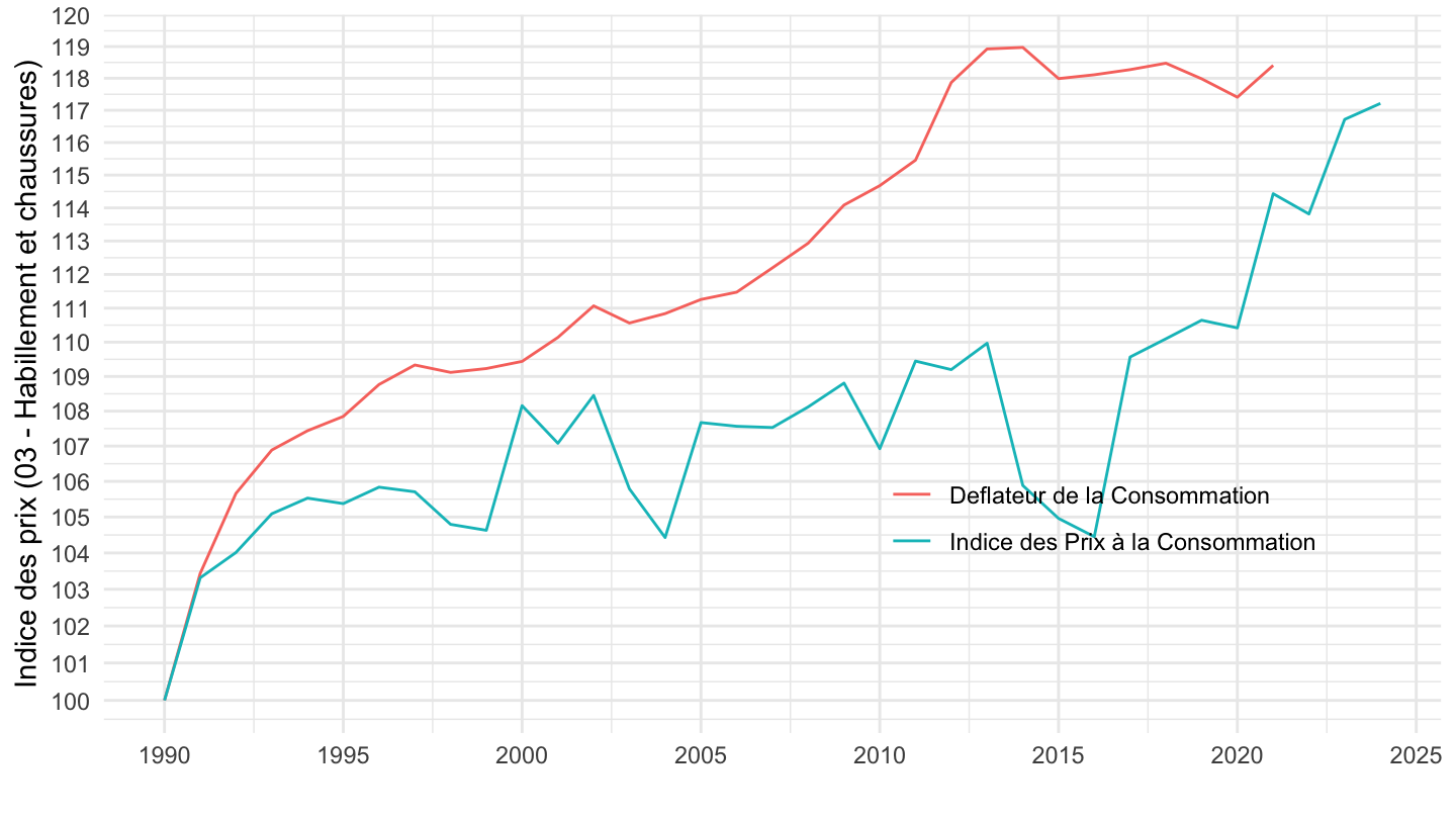
04 - Logement, eau, gaz, électricité et autres combustibles
Code
`conso-eff-fonction` %>%
  filter(fonction == "04",
         variable == "Iprix2014") %>%
  year_to_date2 %>%
  filter(date >= as.Date("1990-01-01")) %>%
  mutate(variable = "Deflateur de la Consommation") %>%
  select(variable, date, value) %>%
  bind_rows(`IPC-2015` %>%
              filter(INDICATEUR == "IPC",
                     MENAGES_IPC == "ENSEMBLE",
                     COICOP2016 %in% c("04"),
                     FREQ == "M",
                     REF_AREA == "FE",
                     NATURE == "INDICE") %>%
              month_to_date %>%
              filter(month(date) == 1) %>%
              select(date, value = OBS_VALUE) %>%
              mutate(variable = "Indice des Prix à la Consommation")) %>%
  group_by(variable) %>%
  mutate(value = 100*value/value[date == as.Date("1990-01-01")]) %>%
  ggplot() + ylab("Indice des prix (04 - Logement)") + xlab("") + theme_minimal() +
  geom_line(aes(x = date, y = value, color = variable)) +

  scale_x_date(breaks = seq(1920, 2025, 5) %>% paste0("-01-01") %>% as.Date,
               labels = date_format("%Y")) +
  theme(legend.position = c(0.75, 0.3),
        legend.title = element_blank()) +
  scale_y_log10(breaks = seq(0, 500, 10),
                     labels = dollar_format(accuracy = 1, prefix = ""))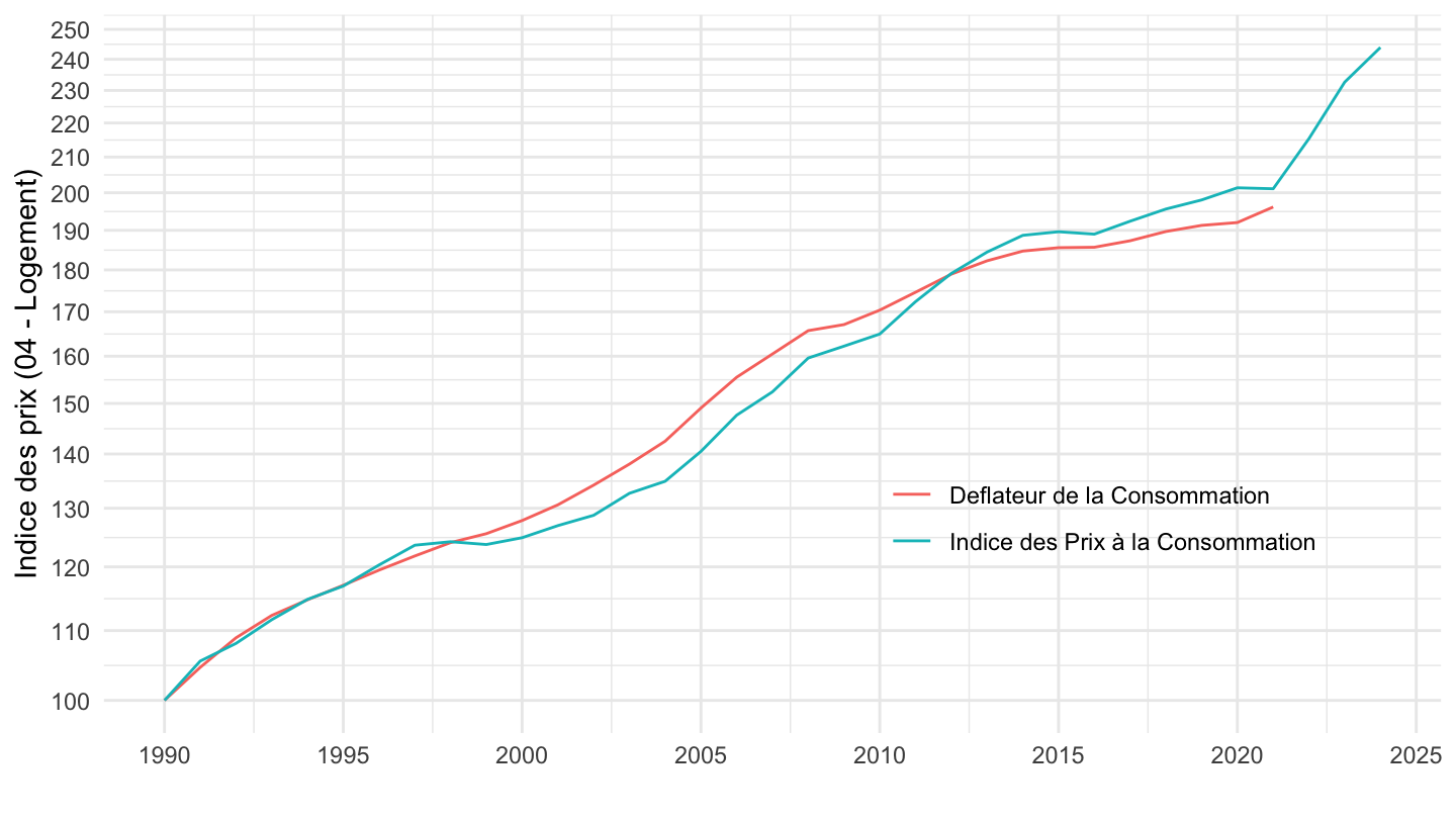
05 - Meubles, articles de ménage et entretien courant de l’habitation
Code
`conso-eff-fonction` %>%
  filter(fonction == "05",
         variable == "Iprix2014") %>%
  year_to_date2 %>%
  filter(date >= as.Date("1990-01-01")) %>%
  mutate(variable = "Deflateur de la Consommation") %>%
  select(variable, date, value) %>%
  bind_rows(`IPC-2015` %>%
              filter(INDICATEUR == "IPC",
                     MENAGES_IPC == "ENSEMBLE",
                     COICOP2016 %in% c("05"),
                     FREQ == "M",
                     REF_AREA == "FE",
                     NATURE == "INDICE") %>%
              month_to_date %>%
              filter(month(date) == 1) %>%
              select(date, value = OBS_VALUE) %>%
              mutate(variable = "Indice des Prix à la Consommation")) %>%
  group_by(variable) %>%
  mutate(value = 100*value/value[date == as.Date("1990-01-01")]) %>%
  ggplot() + ylab("Indice des prix (05 - Meubles)") + xlab("") + theme_minimal() +
  geom_line(aes(x = date, y = value, color = variable)) +

  scale_x_date(breaks = seq(1920, 2025, 5) %>% paste0("-01-01") %>% as.Date,
               labels = date_format("%Y")) +
  theme(legend.position = c(0.75, 0.3),
        legend.title = element_blank()) +
  scale_y_log10(breaks = seq(0, 500, 5),
                     labels = dollar_format(accuracy = 1, prefix = ""))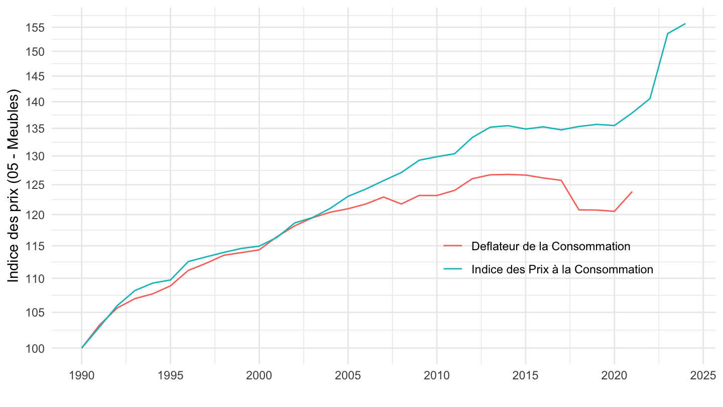
06 - Santé
Code
`conso-eff-fonction` %>%
  filter(fonction == "06",
         variable == "Iprix2014") %>%
  year_to_date2 %>%
  filter(date >= as.Date("1990-01-01")) %>%
  mutate(variable = "Deflateur de la Consommation") %>%
  select(variable, date, value) %>%
  bind_rows(`IPC-2015` %>%
              filter(INDICATEUR == "IPC",
                     MENAGES_IPC == "ENSEMBLE",
                     COICOP2016 %in% c("06"),
                     FREQ == "M",
                     REF_AREA == "FE",
                     NATURE == "INDICE") %>%
              month_to_date %>%
              filter(month(date) == 1) %>%
              select(date, value = OBS_VALUE) %>%
              mutate(variable = "Indice des Prix à la Consommation")) %>%
  group_by(variable) %>%
  mutate(value = 100*value/value[date == as.Date("1990-01-01")]) %>%
  ggplot() + ylab("Indice des prix (06 - Santé)") + xlab("") + theme_minimal() +
  geom_line(aes(x = date, y = value, color = variable)) +

  scale_x_date(breaks = seq(1920, 2025, 5) %>% paste0("-01-01") %>% as.Date,
               labels = date_format("%Y")) +
  theme(legend.position = c(0.75, 0.3),
        legend.title = element_blank()) +
  scale_y_log10(breaks = seq(0, 500, 1),
                     labels = dollar_format(accuracy = 1, prefix = ""))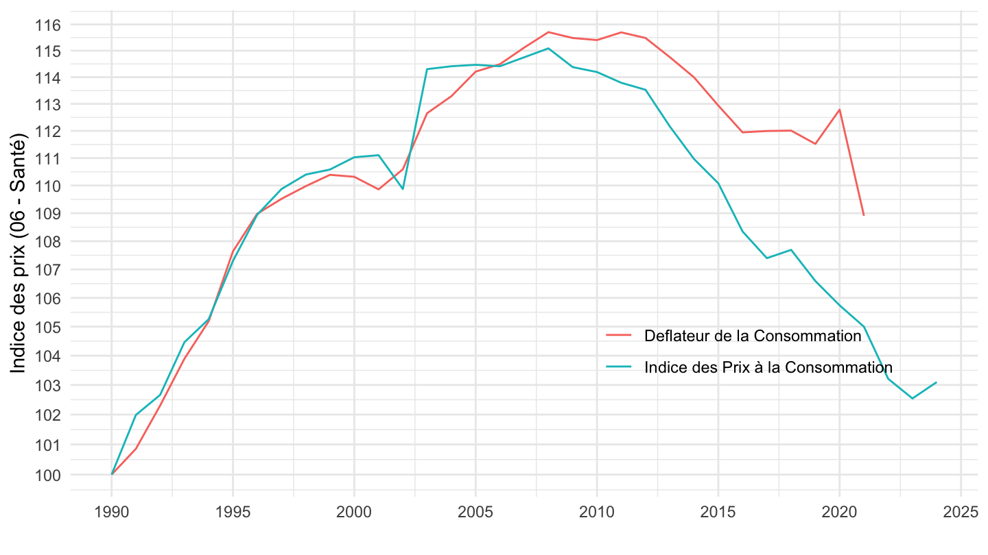
07 - Transports
Code
`conso-eff-fonction` %>%
  filter(fonction == "07",
         variable == "Iprix2014") %>%
  year_to_date2 %>%
  filter(date >= as.Date("1990-01-01")) %>%
  mutate(variable = "Deflateur de la Consommation") %>%
  select(variable, date, value) %>%
  bind_rows(`IPC-2015` %>%
              filter(INDICATEUR == "IPC",
                     MENAGES_IPC == "ENSEMBLE",
                     COICOP2016 %in% c("07"),
                     FREQ == "M",
                     REF_AREA == "FE",
                     NATURE == "INDICE") %>%
              month_to_date %>%
              filter(month(date) == 1) %>%
              select(date, value = OBS_VALUE) %>%
              mutate(variable = "Indice des Prix à la Consommation")) %>%
  group_by(variable) %>%
  mutate(value = 100*value/value[date == as.Date("1990-01-01")]) %>%
  ggplot() + ylab("Indice des prix (07 - Transports)") + xlab("") + theme_minimal() +
  geom_line(aes(x = date, y = value, color = variable)) +

  scale_x_date(breaks = seq(1920, 2025, 5) %>% paste0("-01-01") %>% as.Date,
               labels = date_format("%Y")) +
  theme(legend.position = c(0.75, 0.3),
        legend.title = element_blank()) +
  scale_y_log10(breaks = seq(0, 500, 10),
                     labels = dollar_format(accuracy = 1, prefix = ""))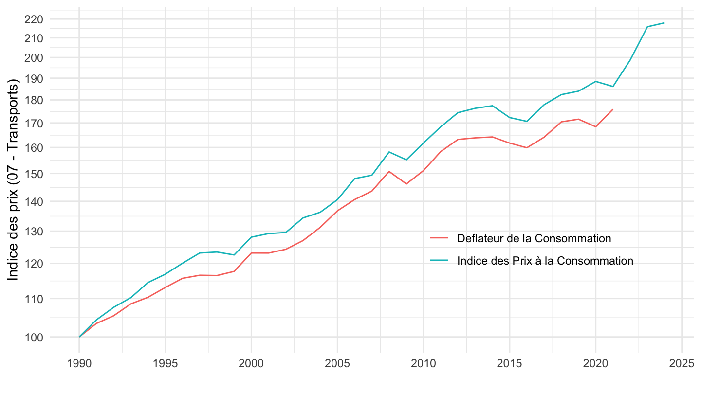
08 - Communications
All
Code
`conso-eff-fonction` %>%
  filter(fonction == "08",
         variable == "Iprix2014") %>%
  year_to_date2 %>%
  filter(date >= as.Date("1990-01-01")) %>%
  mutate(variable = "Deflateur de la Consommation") %>%
  select(variable, date, value) %>%
  bind_rows(`IPC-2015` %>%
              filter(INDICATEUR == "IPC",
                     MENAGES_IPC == "ENSEMBLE",
                     COICOP2016 %in% c("08"),
                     FREQ == "M",
                     REF_AREA == "FE",
                     NATURE == "INDICE") %>%
              month_to_date %>%
              filter(month(date) == 1) %>%
              select(date, value = OBS_VALUE) %>%
              mutate(variable = "Indice des Prix à la Consommation")) %>%
  group_by(variable) %>%
  mutate(value = 100*value/value[date == as.Date("1990-01-01")]) %>%
  ggplot() + ylab("Indice des prix (08 - Communications)") + xlab("") + theme_minimal() +
  geom_line(aes(x = date, y = value, color = variable)) +

  scale_x_date(breaks = seq(1920, 2025, 5) %>% paste0("-01-01") %>% as.Date,
               labels = date_format("%Y")) +
  theme(legend.position = c(0.3, 0.3),
        legend.title = element_blank()) +
  scale_y_log10(breaks = seq(0, 500, 10),
                     labels = dollar_format(accuracy = 1, prefix = ""))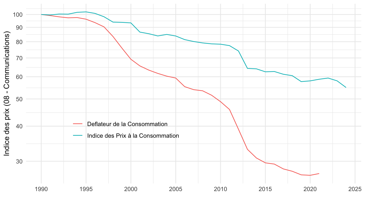
1996
Code
`conso-eff-fonction` %>%
  filter(fonction == "08",
         variable == "Iprix2014") %>%
  year_to_date2 %>%
  filter(date >= as.Date("1996-01-01")) %>%
  mutate(variable = "Deflateur de la Consommation") %>%
  select(variable, date, value) %>%
  bind_rows(`IPC-2015` %>%
              filter(INDICATEUR == "IPC",
                     MENAGES_IPC == "ENSEMBLE",
                     COICOP2016 %in% c("08"),
                     FREQ == "M",
                     REF_AREA == "FE",
                     NATURE == "INDICE") %>%
              month_to_date %>%
              filter(month(date) == 1,
                     date >= as.Date("1996-01-01")) %>%
              select(date, value = OBS_VALUE) %>%
              mutate(variable = "Indice des Prix à la Consommation")) %>%
  group_by(variable) %>%
  mutate(value = 100*value/value[date == as.Date("1996-01-01")]) %>%
  ggplot() + ylab("Indice des prix (08 - Communications)") + xlab("") + theme_minimal() +
  geom_line(aes(x = date, y = value, color = variable)) +

  scale_x_date(breaks = seq(1920, 2025, 2) %>% paste0("-01-01") %>% as.Date,
               labels = date_format("%Y")) +
  theme(legend.position = c(0.3, 0.3),
        legend.title = element_blank()) +
  scale_y_log10(breaks = seq(0, 500, 10),
                     labels = dollar_format(accuracy = 1, prefix = ""))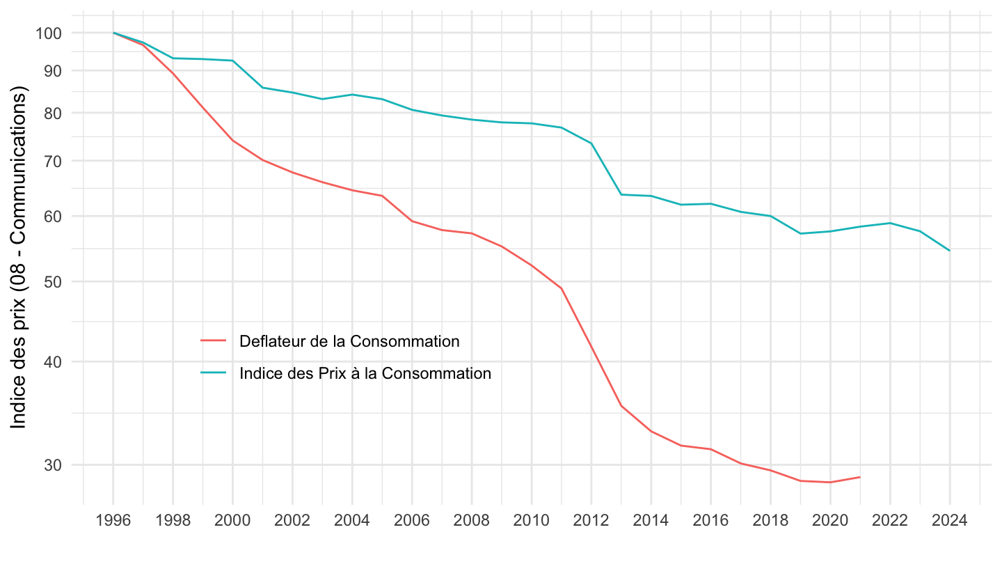
09 - Loisirs et culture
Code
`conso-eff-fonction` %>%
  filter(fonction == "09",
         variable == "Iprix2014") %>%
  year_to_date2 %>%
  filter(date >= as.Date("1990-01-01")) %>%
  mutate(variable = "Deflateur de la Consommation") %>%
  select(variable, date, value) %>%
  bind_rows(`IPC-2015` %>%
              filter(INDICATEUR == "IPC",
                     MENAGES_IPC == "ENSEMBLE",
                     COICOP2016 %in% c("09"),
                     FREQ == "M",
                     REF_AREA == "FE",
                     NATURE == "INDICE") %>%
              month_to_date %>%
              filter(month(date) == 1) %>%
              select(date, value = OBS_VALUE) %>%
              mutate(variable = "Indice des Prix à la Consommation")) %>%
  group_by(variable) %>%
  mutate(value = 100*value/value[date == as.Date("1990-01-01")]) %>%
  ggplot() + ylab("Indice des prix (09 - Loisirs et culture)") + xlab("") + theme_minimal() +
  geom_line(aes(x = date, y = value, color = variable)) +

  scale_x_date(breaks = seq(1920, 2025, 5) %>% paste0("-01-01") %>% as.Date,
               labels = date_format("%Y")) +
  theme(legend.position = c(0.75, 0.3),
        legend.title = element_blank()) +
  scale_y_log10(breaks = seq(0, 500, 10),
                     labels = dollar_format(accuracy = 1, prefix = ""))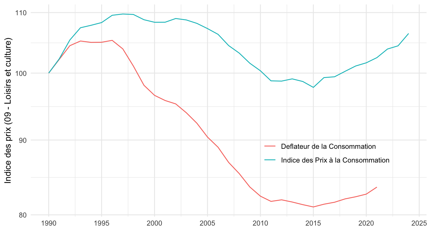
10 - Éducation
Code
`conso-eff-fonction` %>%
  filter(fonction == "10",
         variable == "Iprix2014") %>%
  year_to_date2 %>%
  filter(date >= as.Date("1990-01-01")) %>%
  mutate(variable = "Deflateur de la Consommation") %>%
  select(variable, date, value) %>%
  bind_rows(`IPC-2015` %>%
              filter(INDICATEUR == "IPC",
                     MENAGES_IPC == "ENSEMBLE",
                     COICOP2016 %in% c("10"),
                     FREQ == "M",
                     REF_AREA == "FE",
                     NATURE == "INDICE") %>%
              month_to_date %>%
              filter(month(date) == 1) %>%
              select(date, value = OBS_VALUE) %>%
              mutate(variable = "Indice des Prix à la Consommation")) %>%
  group_by(variable) %>%
  mutate(value = 100*value/value[date == as.Date("1990-01-01")]) %>%
  ggplot() + ylab("Indice des prix") + xlab("") + theme_minimal() +
  geom_line(aes(x = date, y = value, color = variable)) +

  scale_x_date(breaks = seq(1920, 2025, 5) %>% paste0("-01-01") %>% as.Date,
               labels = date_format("%Y")) +
  theme(legend.position = c(0.75, 0.3),
        legend.title = element_blank()) +
  scale_y_log10(breaks = seq(0, 500, 10),
                     labels = dollar_format(accuracy = 1, prefix = ""))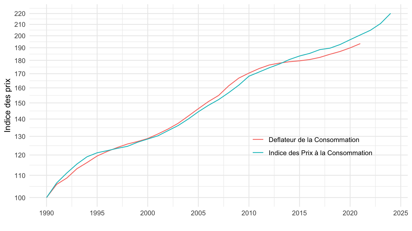
11 - Hôtels, cafés et restaurants
Code
`conso-eff-fonction` %>%
  filter(fonction == "11",
         variable == "Iprix2014") %>%
  year_to_date2 %>%
  filter(date >= as.Date("1990-01-01")) %>%
  mutate(variable = "Deflateur de la Consommation") %>%
  select(variable, date, value) %>%
  bind_rows(`IPC-2015` %>%
              filter(INDICATEUR == "IPC",
                     MENAGES_IPC == "ENSEMBLE",
                     COICOP2016 %in% c("11"),
                     FREQ == "M",
                     REF_AREA == "FE",
                     NATURE == "INDICE") %>%
              month_to_date %>%
              filter(month(date) == 1) %>%
              select(date, value = OBS_VALUE) %>%
              mutate(variable = "Indice des Prix à la Consommation")) %>%
  group_by(variable) %>%
  mutate(value = 100*value/value[date == as.Date("1990-01-01")]) %>%
  ggplot() + ylab("Indice des prix") + xlab("") + theme_minimal() +
  geom_line(aes(x = date, y = value, color = variable)) +

  scale_x_date(breaks = seq(1920, 2025, 5) %>% paste0("-01-01") %>% as.Date,
               labels = date_format("%Y")) +
  theme(legend.position = c(0.75, 0.3),
        legend.title = element_blank()) +
  scale_y_log10(breaks = seq(0, 500, 10),
                     labels = dollar_format(accuracy = 1, prefix = ""))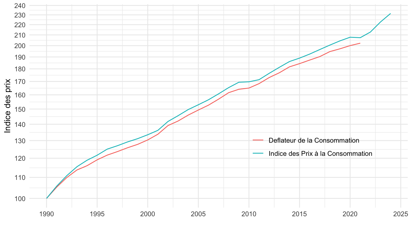
12 - Biens et services divers
Code
`conso-eff-fonction` %>%
  filter(fonction == "12",
         variable == "Iprix2014") %>%
  year_to_date2 %>%
  filter(date >= as.Date("1990-01-01")) %>%
  mutate(variable = "Deflateur de la Consommation") %>%
  select(variable, date, value) %>%
  bind_rows(`IPC-2015` %>%
              filter(INDICATEUR == "IPC",
                     MENAGES_IPC == "ENSEMBLE",
                     COICOP2016 %in% c("12"),
                     FREQ == "M",
                     REF_AREA == "FE",
                     NATURE == "INDICE") %>%
              month_to_date %>%
              filter(month(date) == 1) %>%
              select(date, value = OBS_VALUE) %>%
              mutate(variable = "Indice des Prix à la Consommation")) %>%
  group_by(variable) %>%
  mutate(value = 100*value/value[date == as.Date("1990-01-01")]) %>%
  ggplot() + ylab("Indice des prix") + xlab("") + theme_minimal() +
  geom_line(aes(x = date, y = value, color = variable)) +

  scale_x_date(breaks = seq(1920, 2025, 5) %>% paste0("-01-01") %>% as.Date,
               labels = date_format("%Y")) +
  theme(legend.position = c(0.25, 0.9),
        legend.title = element_blank()) +
  scale_y_log10(breaks = seq(0, 500, 10),
                     labels = dollar_format(accuracy = 1, prefix = ""))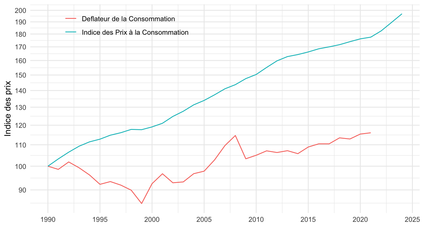
13 - Dépense de consommation finale individualisable des ISBLSM
Code
`conso-eff-fonction` %>%
  filter(fonction == "13",
         variable == "Iprix2014") %>%
  year_to_date2 %>%
  filter(date >= as.Date("1990-01-01")) %>%
  mutate(variable = "Deflateur de la Consommation") %>%
  select(variable, date, value) %>%
  group_by(variable) %>%
  mutate(value = 100*value/value[date == as.Date("1990-01-01")]) %>%
  ggplot() + ylab("Indice des prix") + xlab("") + theme_minimal() +
  geom_line(aes(x = date, y = value, color = variable)) +

  scale_x_date(breaks = seq(1920, 2025, 5) %>% paste0("-01-01") %>% as.Date,
               labels = date_format("%Y")) +
  theme(legend.position = c(0.25, 0.9),
        legend.title = element_blank()) +
  scale_y_log10(breaks = seq(0, 500, 10),
                     labels = dollar_format(accuracy = 1, prefix = ""))
14 - Dépense de consommation finale individualisable des APU
Code
`conso-eff-fonction` %>%
  filter(fonction == "14",
         variable == "Iprix2014") %>%
  year_to_date2 %>%
  filter(date >= as.Date("1990-01-01")) %>%
  mutate(variable = "Deflateur de la Consommation") %>%
  select(variable, date, value) %>%
  group_by(variable) %>%
  mutate(value = 100*value/value[date == as.Date("1990-01-01")]) %>%
  ggplot() + ylab("Indice des prix") + xlab("") + theme_minimal() +
  geom_line(aes(x = date, y = value, color = variable)) +

  scale_x_date(breaks = seq(1920, 2025, 5) %>% paste0("-01-01") %>% as.Date,
               labels = date_format("%Y")) +
  theme(legend.position = c(0.25, 0.9),
        legend.title = element_blank()) +
  scale_y_log10(breaks = seq(0, 500, 10),
                     labels = dollar_format(accuracy = 1, prefix = ""))
15 - Solde territorial
Code
`conso-eff-fonction` %>%
  filter(fonction == "15",
         variable == "Iprix2014") %>%
  year_to_date2 %>%
  filter(date >= as.Date("1990-01-01")) %>%
  mutate(variable = "Deflateur de la Consommation") %>%
  select(variable, date, value) %>%
  group_by(variable) %>%
  mutate(value = 100*value/value[date == as.Date("1990-01-01")]) %>%
  ggplot() + ylab("Indice des prix") + xlab("") + theme_minimal() +
  geom_line(aes(x = date, y = value, color = variable)) +

  scale_x_date(breaks = seq(1920, 2025, 5) %>% paste0("-01-01") %>% as.Date,
               labels = date_format("%Y")) +
  theme(legend.position = c(0.25, 0.9),
        legend.title = element_blank()) +
  scale_y_log10(breaks = seq(0, 500, 10),
                     labels = dollar_format(accuracy = 1, prefix = ""))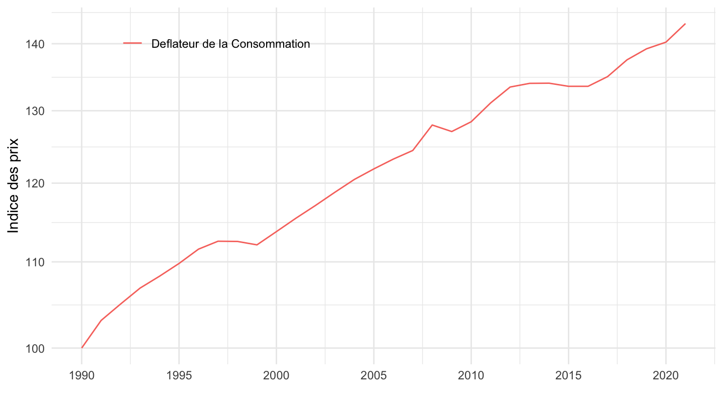
3-digit
02.2 - Tabac
All
Code
`conso-eff-fonction` %>%
  filter(fonction == "02.2",
         variable == "Iprix2014") %>%
  year_to_date2 %>%
  filter(date >= as.Date("1990-01-01")) %>%
  mutate(variable = "Deflateur de la Consommation") %>%
  select(variable, date, value) %>%
  bind_rows(`IPC-2015` %>%
              filter(INDICATEUR == "IPC",
                     MENAGES_IPC == "ENSEMBLE",
                     COICOP2016 %in% c("022"),
                     FREQ == "M",
                     REF_AREA == "FE",
                     NATURE == "INDICE") %>%
              month_to_date %>%
              filter(month(date) == 1) %>%
              select(date, value = OBS_VALUE) %>%
              mutate(variable = "Indice des Prix à la Consommation")) %>%
  group_by(variable) %>%
  mutate(value = 100*value/value[date == as.Date("1990-01-01")]) %>%
  ggplot() + ylab("Indice des prix") + xlab("") + theme_minimal() +
  geom_line(aes(x = date, y = value, color = variable)) +

  scale_x_date(breaks = seq(1920, 2025, 5) %>% paste0("-01-01") %>% as.Date,
               labels = date_format("%Y")) +
  theme(legend.position = c(0.25, 0.9),
        legend.title = element_blank()) +
  scale_y_log10(breaks = seq(0, 800, 50),
                     labels = dollar_format(accuracy = 1, prefix = ""))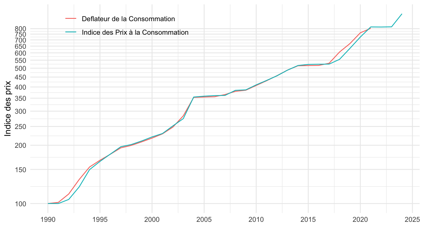
1996-
Code
`conso-eff-fonction` %>%
  filter(fonction == "02.2",
         variable == "Iprix2014") %>%
  year_to_date2 %>%
  filter(date >= as.Date("1996-01-01")) %>%
  mutate(variable = "Deflateur de la Consommation") %>%
  select(variable, date, value) %>%
  bind_rows(`IPC-2015` %>%
              filter(INDICATEUR == "IPC",
                     MENAGES_IPC == "ENSEMBLE",
                     COICOP2016 %in% c("022"),
                     FREQ == "M",
                     REF_AREA == "FE",
                     NATURE == "INDICE") %>%
              month_to_date %>%
              filter(month(date) == 1,
                     date >= as.Date("1996-01-01")) %>%
              select(date, value = OBS_VALUE) %>%
              mutate(variable = "Indice des Prix à la Consommation")) %>%
  group_by(variable) %>%
  mutate(value = 100*value/value[date == as.Date("1996-01-01")]) %>%
  ggplot() + ylab("Indice des prix") + xlab("") + theme_minimal() +
  geom_line(aes(x = date, y = value, color = variable)) +

  scale_x_date(breaks = seq(1920, 2025, 2) %>% paste0("-01-01") %>% as.Date,
               labels = date_format("%Y")) +
  theme(legend.position = c(0.25, 0.9),
        legend.title = element_blank()) +
  scale_y_log10(breaks = seq(0, 800, 50),
                     labels = dollar_format(accuracy = 1, prefix = ""))
02.3 - Bière
Code
`conso-eff-fonction` %>%
  filter(fonction == "02.1.3",
         variable == "Iprix2014") %>%
  year_to_date2 %>%
  filter(date >= as.Date("1990-01-01")) %>%
  mutate(variable = "Deflateur de la Consommation") %>%
  select(variable, date, value) %>%
  bind_rows(`IPC-2015` %>%
              filter(INDICATEUR == "IPC",
                     MENAGES_IPC == "ENSEMBLE",
                     COICOP2016 %in% c("0213"),
                     FREQ == "M",
                     REF_AREA == "FE",
                     NATURE == "INDICE") %>%
              month_to_date %>%
              filter(month(date) == 1) %>%
              select(date, value = OBS_VALUE) %>%
              mutate(variable = "Indice des Prix à la Consommation")) %>%
  group_by(variable) %>%
  mutate(value = 100*value/value[date == as.Date("1990-01-01")]) %>%
  ggplot() + ylab("Indice des prix") + xlab("") + theme_minimal() +
  geom_line(aes(x = date, y = value, color = variable)) +

  scale_x_date(breaks = seq(1920, 2025, 5) %>% paste0("-01-01") %>% as.Date,
               labels = date_format("%Y")) +
  theme(legend.position = c(0.25, 0.9),
        legend.title = element_blank()) +
  scale_y_log10(breaks = seq(0, 800, 10),
                     labels = dollar_format(accuracy = 1, prefix = ""))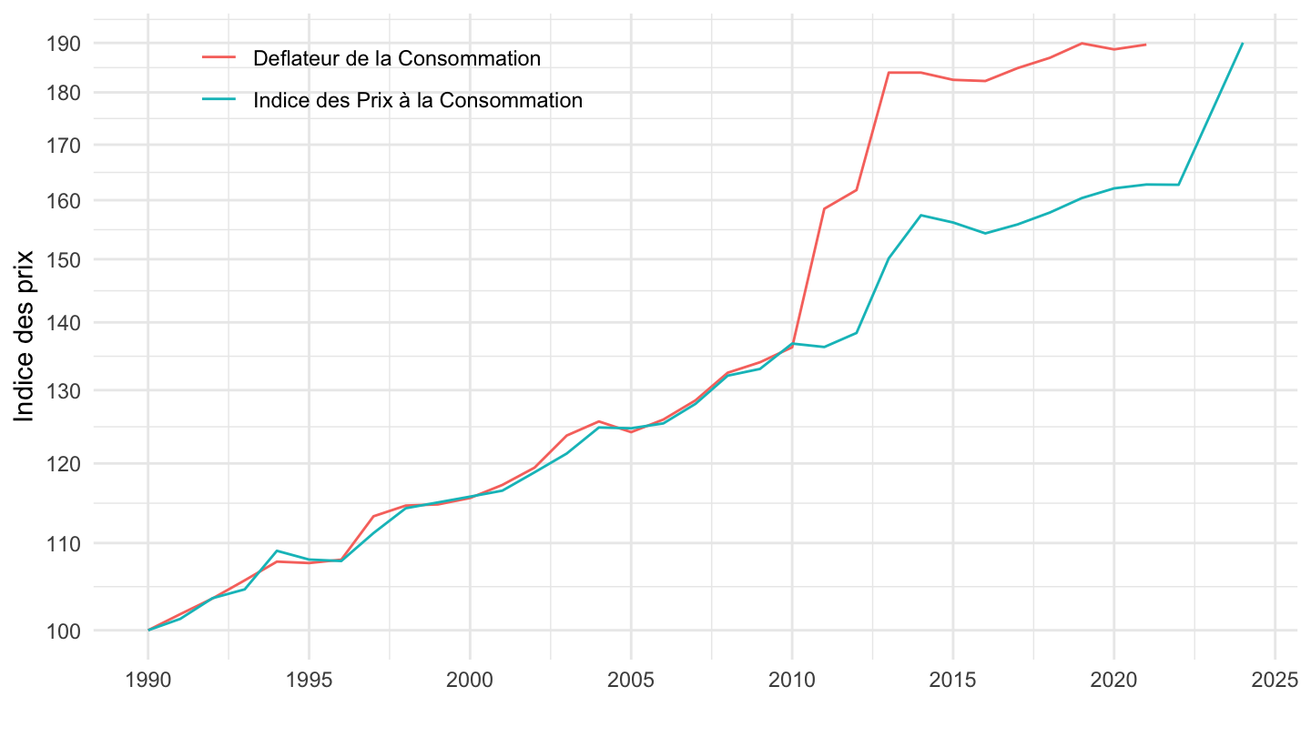
04.1 - Loyers effectifs
Code
`conso-eff-fonction` %>%
  filter(fonction == "04.1",
         variable == "Iprix2014") %>%
  year_to_date2 %>%
  filter(date >= as.Date("1990-01-01")) %>%
  mutate(variable = "Deflateur de la Consommation") %>%
  select(variable, date, value) %>%
  bind_rows(`IPC-2015` %>%
              filter(INDICATEUR == "IPC",
                     MENAGES_IPC == "ENSEMBLE",
                     COICOP2016 %in% c("041"),
                     FREQ == "M",
                     REF_AREA == "FE",
                     NATURE == "INDICE") %>%
              month_to_date %>%
              filter(month(date) == 1) %>%
              select(date, value = OBS_VALUE) %>%
              mutate(variable = "Indice des Prix à la Consommation")) %>%
  group_by(variable) %>%
  mutate(value = 100*value/value[date == as.Date("1990-01-01")]) %>%
  ggplot() + ylab("Indice des prix") + xlab("") + theme_minimal() +
  geom_line(aes(x = date, y = value, color = variable)) +

  scale_x_date(breaks = seq(1920, 2025, 5) %>% paste0("-01-01") %>% as.Date,
               labels = date_format("%Y")) +
  theme(legend.position = c(0.25, 0.9),
        legend.title = element_blank()) +
  scale_y_log10(breaks = seq(0, 500, 10),
                     labels = dollar_format(accuracy = 1, prefix = ""))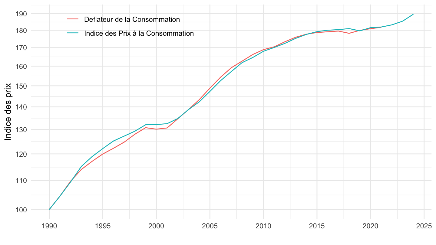
04.3 - Entretien et réparation des logements
Code
`conso-eff-fonction` %>%
  filter(fonction == "04.3",
         variable == "Iprix2014") %>%
  year_to_date2 %>%
  filter(date >= as.Date("1990-01-01")) %>%
  mutate(variable = "Deflateur de la Consommation") %>%
  select(variable, date, value) %>%
  bind_rows(`IPC-2015` %>%
              filter(INDICATEUR == "IPC",
                     MENAGES_IPC == "ENSEMBLE",
                     COICOP2016 %in% c("043"),
                     FREQ == "M",
                     REF_AREA == "FE",
                     NATURE == "INDICE") %>%
              month_to_date %>%
              filter(month(date) == 1) %>%
              select(date, value = OBS_VALUE) %>%
              mutate(variable = "Indice des Prix à la Consommation")) %>%
  group_by(variable) %>%
  mutate(value = 100*value/value[date == as.Date("1990-01-01")]) %>%
  ggplot() + ylab("Indice des prix") + xlab("") + theme_minimal() +
  geom_line(aes(x = date, y = value, color = variable)) +

  scale_x_date(breaks = seq(1920, 2025, 5) %>% paste0("-01-01") %>% as.Date,
               labels = date_format("%Y")) +
  theme(legend.position = c(0.75, 0.9),
        legend.title = element_blank()) +
  scale_y_log10(breaks = seq(0, 500, 10),
                     labels = dollar_format(accuracy = 1, prefix = ""))
04.4 - Autres services liés au logement
Code
`conso-eff-fonction` %>%
  filter(fonction == "04.4",
         variable == "Iprix2014") %>%
  year_to_date2 %>%
  filter(date >= as.Date("1990-01-01")) %>%
  mutate(variable = "Deflateur de la Consommation") %>%
  select(variable, date, value) %>%
  bind_rows(`IPC-2015` %>%
              filter(INDICATEUR == "IPC",
                     MENAGES_IPC == "ENSEMBLE",
                     COICOP2016 %in% c("044"),
                     FREQ == "M",
                     REF_AREA == "FE",
                     NATURE == "INDICE") %>%
              month_to_date %>%
              filter(month(date) == 1) %>%
              select(date, value = OBS_VALUE) %>%
              mutate(variable = "Indice des Prix à la Consommation")) %>%
  group_by(variable) %>%
  mutate(value = 100*value/value[date == as.Date("1990-01-01")]) %>%
  ggplot() + ylab("Indice des prix") + xlab("") + theme_minimal() +
  geom_line(aes(x = date, y = value, color = variable)) +

  scale_x_date(breaks = seq(1920, 2025, 5) %>% paste0("-01-01") %>% as.Date,
               labels = date_format("%Y")) +
  theme(legend.position = c(0.25, 0.9),
        legend.title = element_blank()) +
  scale_y_log10(breaks = seq(0, 500, 10),
                     labels = dollar_format(accuracy = 1, prefix = ""))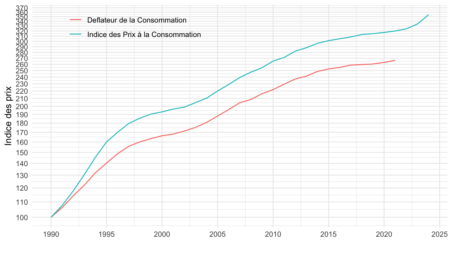
05.1 - Meubles, articles d’ameublement, tapis et autres revêtements de sol
Code
`conso-eff-fonction` %>%
  filter(fonction == "05.1",
         variable == "Iprix2014") %>%
  year_to_date2 %>%
  filter(date >= as.Date("1990-01-01")) %>%
  mutate(variable = "Deflateur de la Consommation") %>%
  select(variable, date, value) %>%
  bind_rows(`IPC-2015` %>%
              filter(INDICATEUR == "IPC",
                     MENAGES_IPC == "ENSEMBLE",
                     COICOP2016 %in% c("051"),
                     FREQ == "M",
                     REF_AREA == "FE",
                     NATURE == "INDICE") %>%
              month_to_date %>%
              filter(month(date) == 1) %>%
              select(date, value = OBS_VALUE) %>%
              mutate(variable = "Indice des Prix à la Consommation")) %>%
  group_by(variable) %>%
  mutate(value = 100*value/value[date == as.Date("1990-01-01")]) %>%
  ggplot() + ylab("Indice des prix") + xlab("") + theme_minimal() +
  geom_line(aes(x = date, y = value, color = variable)) +

  scale_x_date(breaks = seq(1920, 2025, 5) %>% paste0("-01-01") %>% as.Date,
               labels = date_format("%Y")) +
  theme(legend.position = c(0.25, 0.9),
        legend.title = element_blank()) +
  scale_y_log10(breaks = seq(0, 500, 10),
                     labels = dollar_format(accuracy = 1, prefix = ""))
05.2 - Articles de ménage en textile
Code
`conso-eff-fonction` %>%
  filter(fonction == "05.2",
         variable == "Iprix2014") %>%
  year_to_date2 %>%
  filter(date >= as.Date("1990-01-01")) %>%
  mutate(variable = "Deflateur de la Consommation") %>%
  select(variable, date, value) %>%
  bind_rows(`IPC-2015` %>%
              filter(INDICATEUR == "IPC",
                     MENAGES_IPC == "ENSEMBLE",
                     COICOP2016 %in% c("052"),
                     FREQ == "M",
                     REF_AREA == "FE",
                     NATURE == "INDICE") %>%
              month_to_date %>%
              filter(month(date) == 1) %>%
              select(date, value = OBS_VALUE) %>%
              mutate(variable = "Indice des Prix à la Consommation")) %>%
  group_by(variable) %>%
  mutate(value = 100*value/value[date == as.Date("1990-01-01")]) %>%
  ggplot() + ylab("Indice des prix") + xlab("") + theme_minimal() +
  geom_line(aes(x = date, y = value, color = variable)) +

  scale_x_date(breaks = seq(1920, 2025, 5) %>% paste0("-01-01") %>% as.Date,
               labels = date_format("%Y")) +
  theme(legend.position = c(0.25, 0.9),
        legend.title = element_blank()) +
  scale_y_log10(breaks = seq(0, 500, 10),
                     labels = dollar_format(accuracy = 1, prefix = ""))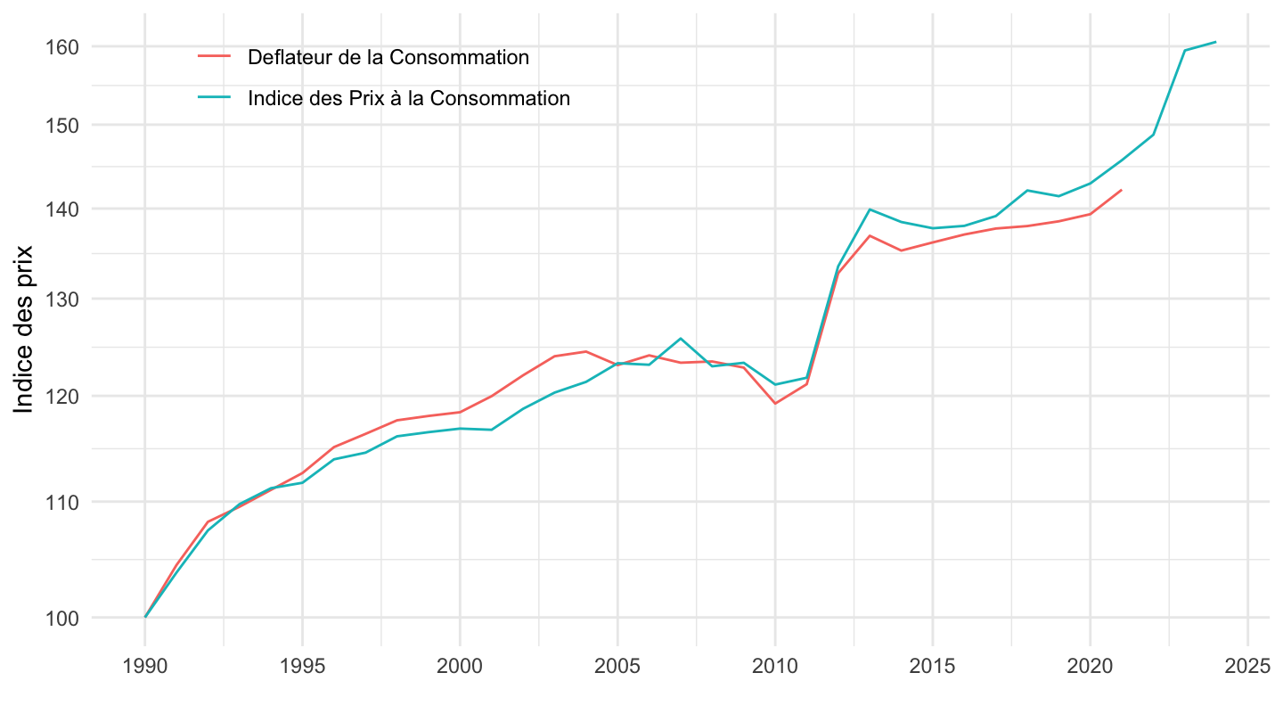
05.3 - Appareils ménagers
Code
`conso-eff-fonction` %>%
  filter(fonction == "05.3",
         variable == "Iprix2014") %>%
  year_to_date2 %>%
  filter(date >= as.Date("1990-01-01")) %>%
  mutate(variable = "Deflateur de la Consommation") %>%
  select(variable, date, value) %>%
  bind_rows(`IPC-2015` %>%
              filter(INDICATEUR == "IPC",
                     MENAGES_IPC == "ENSEMBLE",
                     COICOP2016 %in% c("053"),
                     FREQ == "M",
                     REF_AREA == "FE",
                     NATURE == "INDICE") %>%
              month_to_date %>%
              filter(month(date) == 1) %>%
              select(date, value = OBS_VALUE) %>%
              mutate(variable = "Indice des Prix à la Consommation")) %>%
  group_by(variable) %>%
  mutate(value = 100*value/value[date == as.Date("1990-01-01")]) %>%
  ggplot() + ylab("Indice des prix") + xlab("") + theme_minimal() +
  geom_line(aes(x = date, y = value, color = variable)) +

  scale_x_date(breaks = seq(1920, 2025, 5) %>% paste0("-01-01") %>% as.Date,
               labels = date_format("%Y")) +
  theme(legend.position = c(0.25, 0.2),
        legend.title = element_blank()) +
  scale_y_log10(breaks = seq(0, 500, 10),
                     labels = dollar_format(accuracy = 1, prefix = ""))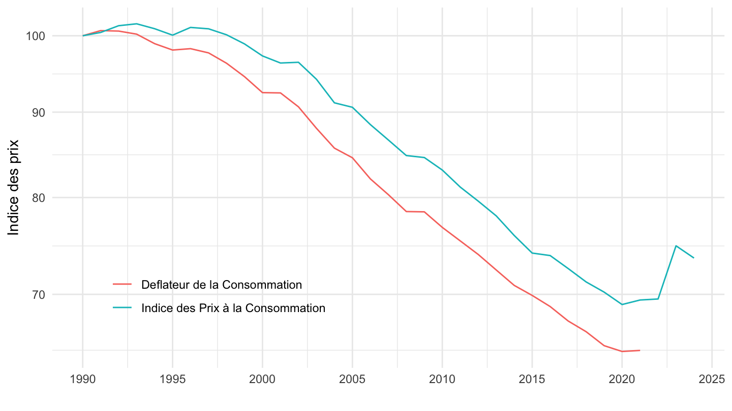
05.4 - Verrerie, vaisselle et ustensiles de ménage
Code
`conso-eff-fonction` %>%
  filter(fonction == "05.4",
         variable == "Iprix2014") %>%
  year_to_date2 %>%
  filter(date >= as.Date("1990-01-01")) %>%
  mutate(variable = "Deflateur de la Consommation") %>%
  select(variable, date, value) %>%
  bind_rows(`IPC-2015` %>%
              filter(INDICATEUR == "IPC",
                     MENAGES_IPC == "ENSEMBLE",
                     COICOP2016 %in% c("054"),
                     FREQ == "M",
                     REF_AREA == "FE",
                     NATURE == "INDICE") %>%
              month_to_date %>%
              filter(month(date) == 1) %>%
              select(date, value = OBS_VALUE) %>%
              mutate(variable = "Indice des Prix à la Consommation")) %>%
  group_by(variable) %>%
  mutate(value = 100*value/value[date == as.Date("1990-01-01")]) %>%
  ggplot() + ylab("Indice des prix") + xlab("") + theme_minimal() +
  geom_line(aes(x = date, y = value, color = variable)) +

  scale_x_date(breaks = seq(1920, 2025, 5) %>% paste0("-01-01") %>% as.Date,
               labels = date_format("%Y")) +
  theme(legend.position = c(0.25, 0.9),
        legend.title = element_blank()) +
  scale_y_log10(breaks = seq(0, 500, 10),
                     labels = dollar_format(accuracy = 1, prefix = ""))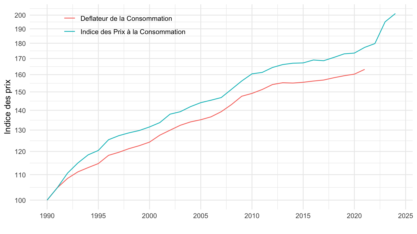
05.5 - Outillage et autre matériel pour la maison et le jardin
Code
`conso-eff-fonction` %>%
  filter(fonction == "05.5",
         variable == "Iprix2014") %>%
  year_to_date2 %>%
  filter(date >= as.Date("1990-01-01")) %>%
  mutate(variable = "Deflateur de la Consommation") %>%
  select(variable, date, value) %>%
  bind_rows(`IPC-2015` %>%
              filter(INDICATEUR == "IPC",
                     MENAGES_IPC == "ENSEMBLE",
                     COICOP2016 %in% c("055"),
                     FREQ == "M",
                     REF_AREA == "FE",
                     NATURE == "INDICE") %>%
              month_to_date %>%
              filter(month(date) == 1) %>%
              select(date, value = OBS_VALUE) %>%
              mutate(variable = "Indice des Prix à la Consommation")) %>%
  group_by(variable) %>%
  mutate(value = 100*value/value[date == as.Date("1990-01-01")]) %>%
  ggplot() + ylab("Indice des prix") + xlab("") + theme_minimal() +
  geom_line(aes(x = date, y = value, color = variable)) +

  scale_x_date(breaks = seq(1920, 2025, 5) %>% paste0("-01-01") %>% as.Date,
               labels = date_format("%Y")) +
  theme(legend.position = c(0.25, 0.9),
        legend.title = element_blank()) +
  scale_y_log10(breaks = seq(0, 500, 10),
                     labels = dollar_format(accuracy = 1, prefix = ""))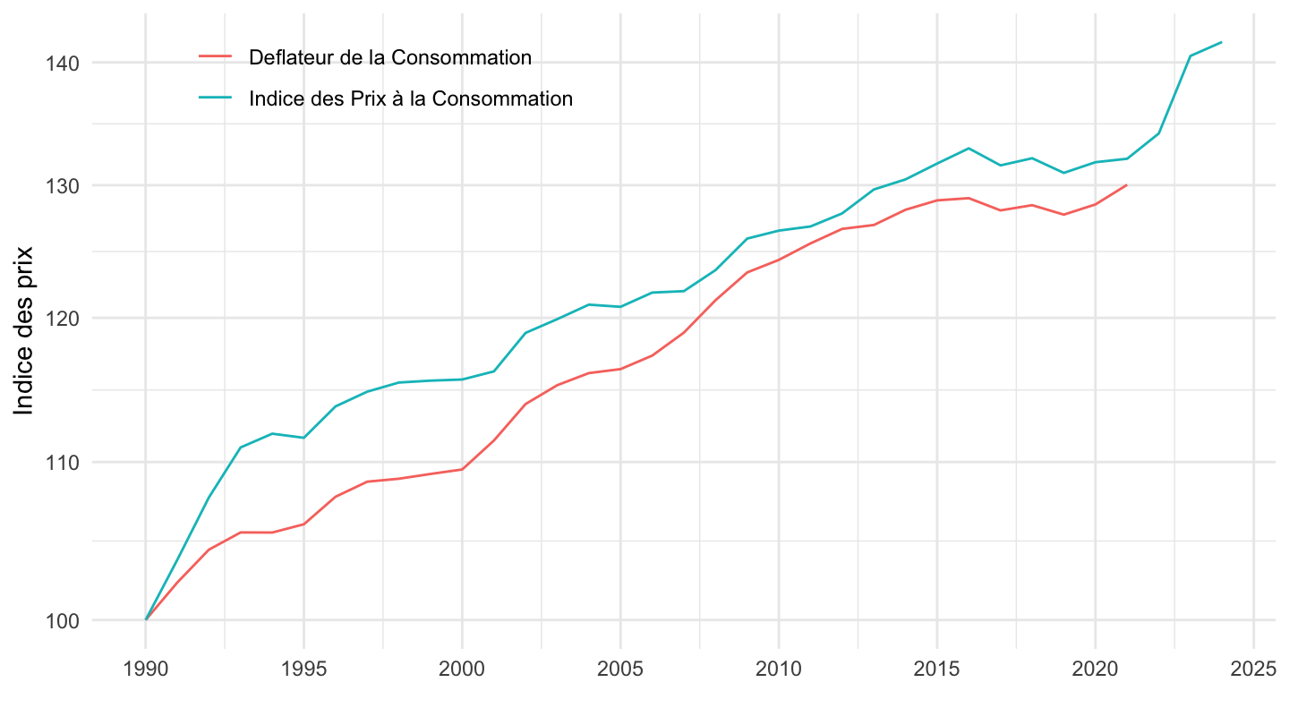
05.6 - Biens et services pour l’entretien courant du foyer
Code
`conso-eff-fonction` %>%
  filter(fonction == "05.6",
         variable == "Iprix2014") %>%
  year_to_date2 %>%
  filter(date >= as.Date("1990-01-01")) %>%
  mutate(variable = "Deflateur de la Consommation") %>%
  select(variable, date, value) %>%
  bind_rows(`IPC-2015` %>%
              filter(INDICATEUR == "IPC",
                     MENAGES_IPC == "ENSEMBLE",
                     COICOP2016 %in% c("056"),
                     FREQ == "M",
                     REF_AREA == "FE",
                     NATURE == "INDICE") %>%
              month_to_date %>%
              filter(month(date) == 1) %>%
              select(date, value = OBS_VALUE) %>%
              mutate(variable = "Indice des Prix à la Consommation")) %>%
  group_by(variable) %>%
  mutate(value = 100*value/value[date == as.Date("1990-01-01")]) %>%
  ggplot() + ylab("Indice des prix") + xlab("") + theme_minimal() +
  geom_line(aes(x = date, y = value, color = variable)) +

  scale_x_date(breaks = seq(1920, 2025, 5) %>% paste0("-01-01") %>% as.Date,
               labels = date_format("%Y")) +
  theme(legend.position = c(0.25, 0.9),
        legend.title = element_blank()) +
  scale_y_log10(breaks = seq(0, 500, 10),
                     labels = dollar_format(accuracy = 1, prefix = ""))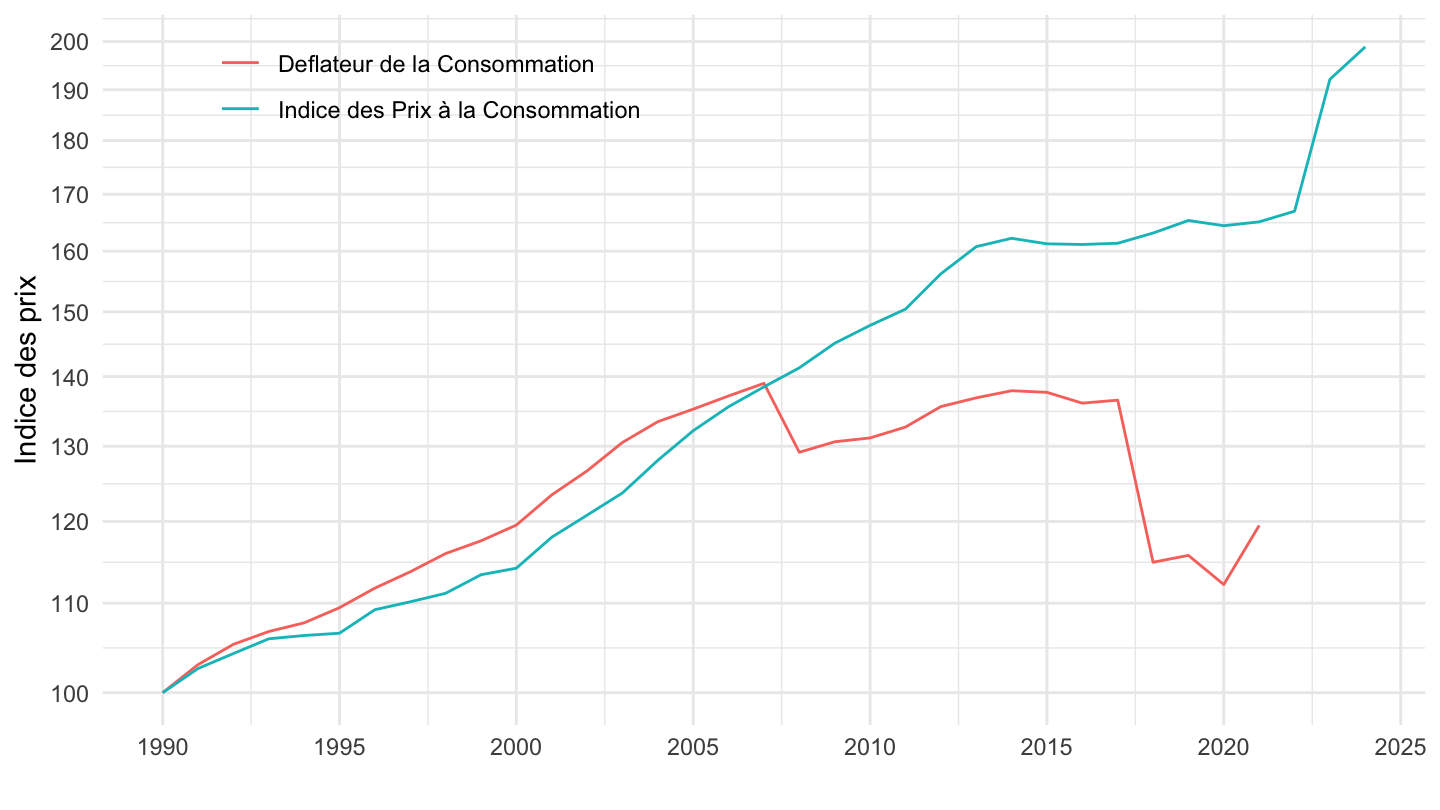
07.2 - Dépenses d’utilisation des véhicules
Code
`conso-eff-fonction` %>%
  filter(fonction == "07.2",
         variable == "Iprix2014") %>%
  year_to_date2 %>%
  filter(date >= as.Date("1990-01-01")) %>%
  mutate(variable = "Deflateur de la Consommation") %>%
  select(variable, date, value) %>%
  bind_rows(`IPC-2015` %>%
              filter(INDICATEUR == "IPC",
                     MENAGES_IPC == "ENSEMBLE",
                     COICOP2016 %in% c("072"),
                     FREQ == "M",
                     REF_AREA == "FE",
                     NATURE == "INDICE") %>%
              month_to_date %>%
              filter(month(date) == 1) %>%
              select(date, value = OBS_VALUE) %>%
              mutate(variable = "Indice des Prix à la Consommation")) %>%
  group_by(variable) %>%
  mutate(value = 100*value/value[date == as.Date("1990-01-01")]) %>%
  ggplot() + ylab("Indice des prix") + xlab("") + theme_minimal() +
  geom_line(aes(x = date, y = value, color = variable)) +

  scale_x_date(breaks = seq(1920, 2025, 5) %>% paste0("-01-01") %>% as.Date,
               labels = date_format("%Y")) +
  theme(legend.position = c(0.25, 0.9),
        legend.title = element_blank()) +
  scale_y_log10(breaks = seq(0, 500, 10),
                     labels = dollar_format(accuracy = 1, prefix = ""))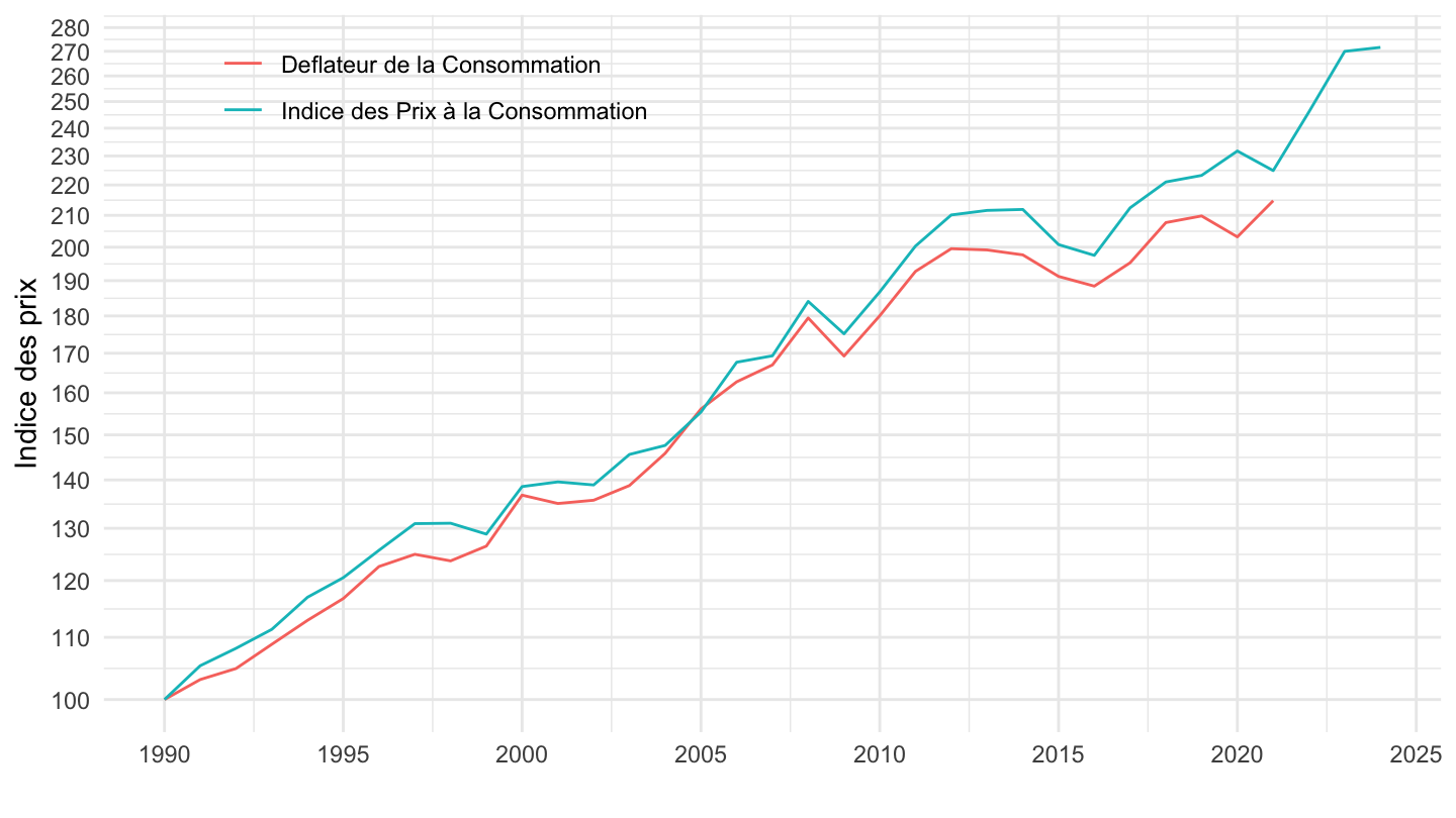
08.1 - Services postaux
Code
`conso-eff-fonction` %>%
  filter(fonction == "08.1",
         variable == "Iprix2014") %>%
  year_to_date2 %>%
  filter(date >= as.Date("1990-01-01")) %>%
  mutate(variable = "Deflateur de la Consommation") %>%
  select(variable, date, value) %>%
  bind_rows(`IPC-2015` %>%
              filter(INDICATEUR == "IPC",
                     MENAGES_IPC == "ENSEMBLE",
                     COICOP2016 %in% c("081"),
                     FREQ == "M",
                     REF_AREA == "FE",
                     NATURE == "INDICE") %>%
              month_to_date %>%
              filter(month(date) == 1) %>%
              select(date, value = OBS_VALUE) %>%
              mutate(variable = "Indice des Prix à la Consommation")) %>%
  group_by(variable) %>%
  mutate(value = 100*value/value[date == as.Date("1990-01-01")]) %>%
  ggplot() + ylab("Indice des prix") + xlab("") + theme_minimal() +
  geom_line(aes(x = date, y = value, color = variable)) +

  scale_x_date(breaks = seq(1920, 2025, 5) %>% paste0("-01-01") %>% as.Date,
               labels = date_format("%Y")) +
  theme(legend.position = c(0.75, 0.9),
        legend.title = element_blank()) +
  scale_y_log10(breaks = seq(0, 500, 10),
                     labels = dollar_format(accuracy = 1, prefix = ""))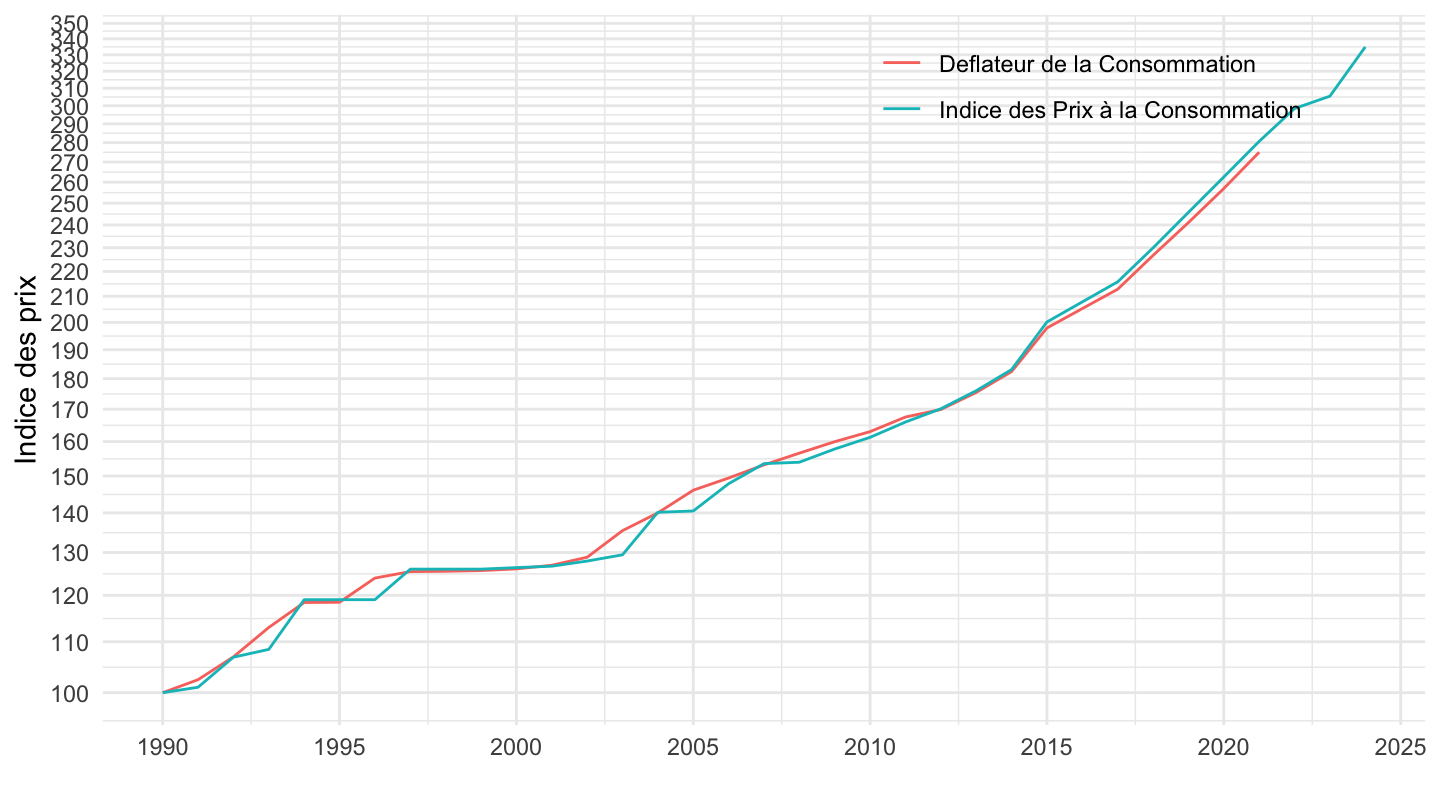
08.2 - Matériel de téléphonie et de télécopie
1990-
Code
`conso-eff-fonction` %>%
  filter(fonction == "08.2",
         variable == "Iprix2014") %>%
  year_to_date2 %>%
  filter(date >= as.Date("1990-01-01")) %>%
  mutate(variable = "Deflateur de la Consommation") %>%
  select(variable, date, value) %>%
  bind_rows(`IPC-2015` %>%
              filter(INDICATEUR == "IPC",
                     MENAGES_IPC == "ENSEMBLE",
                     COICOP2016 %in% c("082"),
                     FREQ == "M",
                     REF_AREA == "FE",
                     NATURE == "INDICE") %>%
              month_to_date %>%
              filter(month(date) == 1) %>%
              select(date, value = OBS_VALUE) %>%
              mutate(variable = "Indice des Prix à la Consommation")) %>%
  group_by(variable) %>%
  mutate(value = 100*value/value[date == as.Date("1993-01-01")]) %>%
  ggplot() + ylab("Indice des prix (1993=100)") + xlab("") + theme_minimal() +
  geom_line(aes(x = date, y = value, color = variable)) +

  scale_x_date(breaks = seq(1920, 2025, 5) %>% paste0("-01-01") %>% as.Date,
               labels = date_format("%Y")) +
  theme(legend.position = c(0.75, 0.9),
        legend.title = element_blank()) +
  scale_y_log10(breaks = c(1, 2, 3, 5, 8, 10, 20, 30, 50, 100),
                     labels = dollar_format(accuracy = 1, prefix = ""))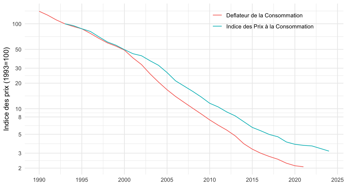
1996-
Code
`conso-eff-fonction` %>%
  filter(fonction == "08.2",
         variable == "Iprix2014") %>%
  year_to_date2 %>%
  filter(date >= as.Date("1996-01-01")) %>%
  mutate(variable = "Deflateur de la Consommation") %>%
  select(variable, date, value) %>%
  bind_rows(`IPC-2015` %>%
              filter(INDICATEUR == "IPC",
                     MENAGES_IPC == "ENSEMBLE",
                     COICOP2016 %in% c("082"),
                     FREQ == "M",
                     REF_AREA == "FE",
                     NATURE == "INDICE") %>%
              month_to_date %>%
              filter(month(date) == 1,
                     date >= as.Date("1996-01-01")) %>%
              select(date, value = OBS_VALUE) %>%
              mutate(variable = "Indice des Prix à la Consommation")) %>%
  group_by(variable) %>%
  mutate(value = 100*value/value[date == as.Date("1996-01-01")]) %>%
  ggplot() + ylab("Indice des prix (1996=100)") + xlab("") + theme_minimal() +
  geom_line(aes(x = date, y = value, color = variable)) +

  scale_x_date(breaks = seq(1920, 2025, 2) %>% paste0("-01-01") %>% as.Date,
               labels = date_format("%Y")) +
  theme(legend.position = c(0.75, 0.9),
        legend.title = element_blank()) +
  scale_y_log10(breaks = c(1, 2, 3, 5, 8, 10, 20, 30, 50, 100),
                     labels = dollar_format(accuracy = 1, prefix = ""))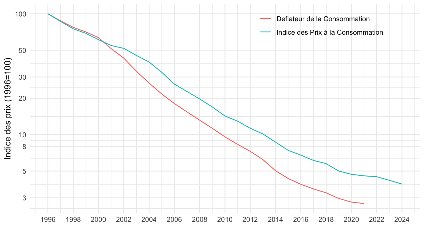
08.3 - Services de télécommunications
Code
`conso-eff-fonction` %>%
  filter(fonction == "08.3",
         variable == "Iprix2014") %>%
  year_to_date2 %>%
  filter(date >= as.Date("1990-01-01")) %>%
  mutate(variable = "Deflateur de la Consommation") %>%
  select(variable, date, value) %>%
  bind_rows(`IPC-2015` %>%
              filter(INDICATEUR == "IPC",
                     MENAGES_IPC == "ENSEMBLE",
                     COICOP2016 %in% c("083"),
                     FREQ == "M",
                     REF_AREA == "FE",
                     NATURE == "INDICE") %>%
              month_to_date %>%
              filter(month(date) == 1) %>%
              select(date, value = OBS_VALUE) %>%
              mutate(variable = "Indice des Prix à la Consommation")) %>%
  group_by(variable) %>%
  mutate(value = 100*value/value[date == as.Date("1990-01-01")]) %>%
  ggplot() + ylab("Indice des prix") + xlab("") + theme_minimal() +
  geom_line(aes(x = date, y = value, color = variable)) +

  scale_x_date(breaks = seq(1920, 2025, 5) %>% paste0("-01-01") %>% as.Date,
               labels = date_format("%Y")) +
  theme(legend.position = c(0.25, 0.2),
        legend.title = element_blank()) +
  scale_y_log10(breaks = seq(0, 500, 10),
                     labels = dollar_format(accuracy = 1, prefix = ""))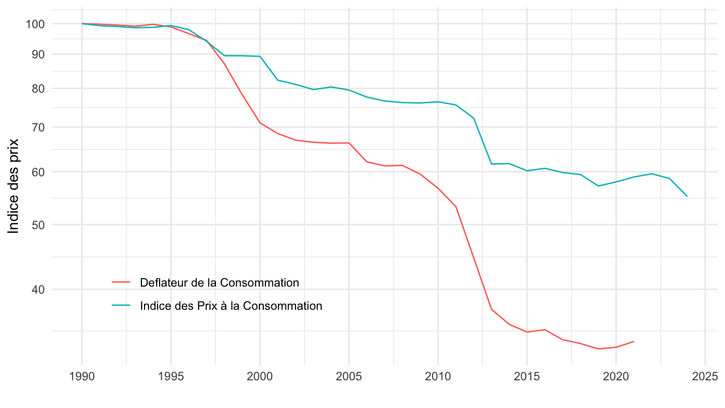
09.1 - Matériel audiovisuel, photographique et informatique
Code
`conso-eff-fonction` %>%
  filter(fonction == "09.1",
         variable == "Iprix2014") %>%
  year_to_date2 %>%
  filter(date >= as.Date("1990-01-01")) %>%
  mutate(variable = "Deflateur de la Consommation") %>%
  select(variable, date, value) %>%
  bind_rows(`IPC-2015` %>%
              filter(INDICATEUR == "IPC",
                     MENAGES_IPC == "ENSEMBLE",
                     COICOP2016 %in% c("091"),
                     FREQ == "M",
                     REF_AREA == "FE",
                     NATURE == "INDICE") %>%
              month_to_date %>%
              filter(month(date) == 1) %>%
              select(date, value = OBS_VALUE) %>%
              mutate(variable = "Indice des Prix à la Consommation")) %>%
  group_by(variable) %>%
  mutate(value = 100*value/value[date == as.Date("1990-01-01")]) %>%
  ggplot() + ylab("Indice des prix") + xlab("") + theme_minimal() +
  geom_line(aes(x = date, y = value, color = variable)) +

  scale_x_date(breaks = seq(1920, 2025, 5) %>% paste0("-01-01") %>% as.Date,
               labels = date_format("%Y")) +
  theme(legend.position = c(0.25, 0.3),
        legend.title = element_blank()) +
  scale_y_log10(breaks = c(seq(0, 500, 10), 15),
                     labels = dollar_format(accuracy = 1, prefix = ""))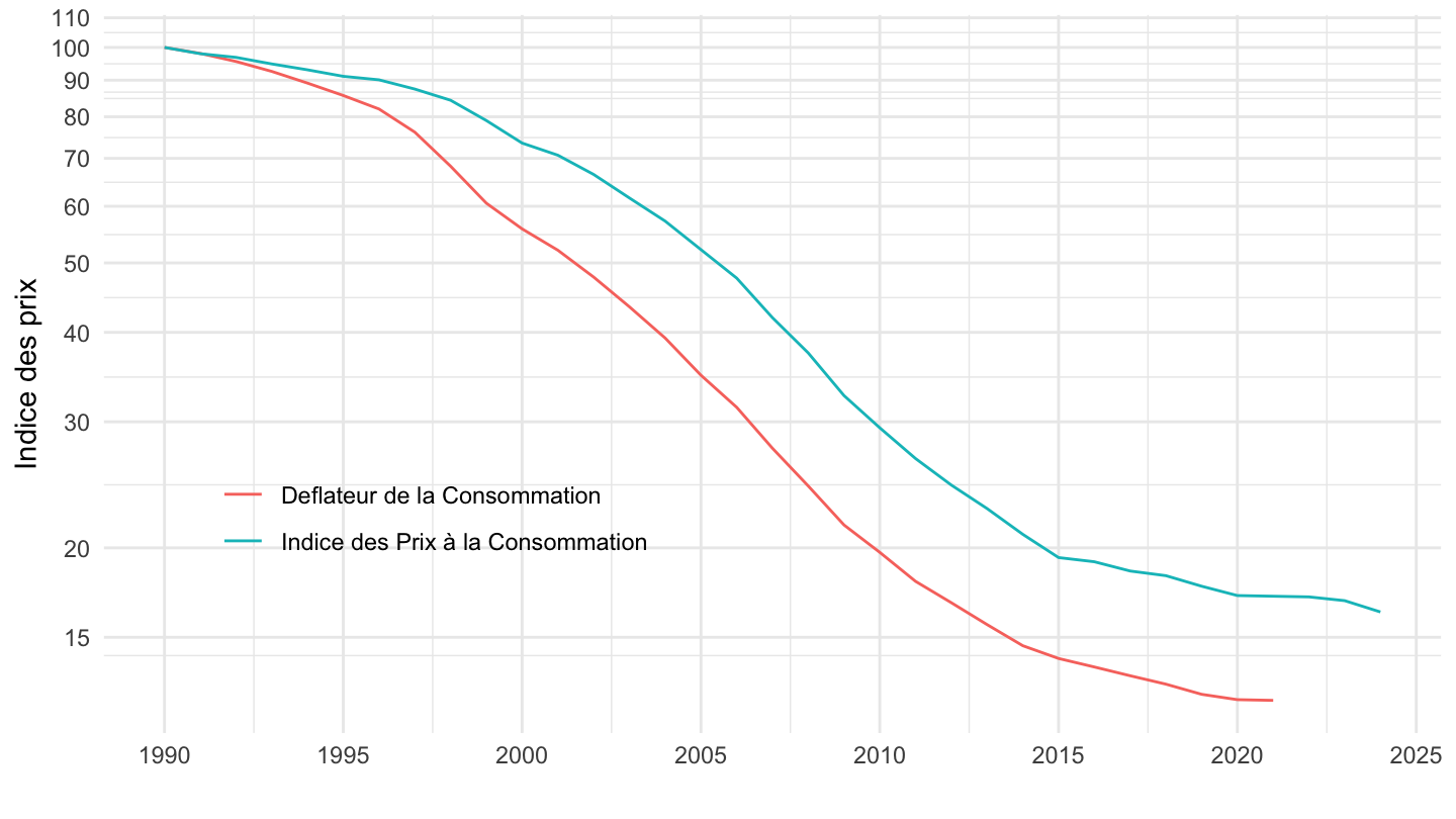
09.2 - Autres biens durables culturels et récréatifs
Code
`conso-eff-fonction` %>%
  filter(fonction == "09.2",
         variable == "Iprix2014") %>%
  year_to_date2 %>%
  filter(date >= as.Date("1990-01-01")) %>%
  mutate(variable = "Deflateur de la Consommation") %>%
  select(variable, date, value) %>%
  bind_rows(`IPC-2015` %>%
              filter(INDICATEUR == "IPC",
                     MENAGES_IPC == "ENSEMBLE",
                     COICOP2016 %in% c("092"),
                     FREQ == "M",
                     REF_AREA == "FE",
                     NATURE == "INDICE") %>%
              month_to_date %>%
              filter(month(date) == 1) %>%
              select(date, value = OBS_VALUE) %>%
              mutate(variable = "Indice des Prix à la Consommation")) %>%
  group_by(variable) %>%
  mutate(value = 100*value/value[date == as.Date("1990-01-01")]) %>%
  ggplot() + ylab("Indice des prix") + xlab("") + theme_minimal() +
  geom_line(aes(x = date, y = value, color = variable)) +

  scale_x_date(breaks = seq(1920, 2025, 5) %>% paste0("-01-01") %>% as.Date,
               labels = date_format("%Y")) +
  theme(legend.position = c(0.25, 0.3),
        legend.title = element_blank()) +
  scale_y_log10(breaks = c(seq(0, 500, 10), 15),
                     labels = dollar_format(accuracy = 1, prefix = ""))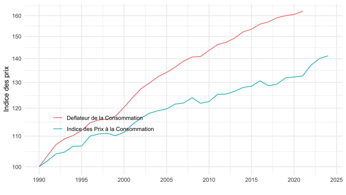
09.3 - Autres articles et matériel de loisirs, de jardinage et animaux de compagnie
Code
`conso-eff-fonction` %>%
  filter(fonction == "09.3",
         variable == "Iprix2014") %>%
  year_to_date2 %>%
  filter(date >= as.Date("1990-01-01")) %>%
  mutate(variable = "Deflateur de la Consommation") %>%
  select(variable, date, value) %>%
  bind_rows(`IPC-2015` %>%
              filter(INDICATEUR == "IPC",
                     MENAGES_IPC == "ENSEMBLE",
                     COICOP2016 %in% c("093"),
                     FREQ == "M",
                     REF_AREA == "FE",
                     NATURE == "INDICE") %>%
              month_to_date %>%
              filter(month(date) == 1) %>%
              select(date, value = OBS_VALUE) %>%
              mutate(variable = "Indice des Prix à la Consommation")) %>%
  group_by(variable) %>%
  mutate(value = 100*value/value[date == as.Date("1990-01-01")]) %>%
  ggplot() + ylab("Indice des prix") + xlab("") + theme_minimal() +
  geom_line(aes(x = date, y = value, color = variable)) +

  scale_x_date(breaks = seq(1920, 2025, 5) %>% paste0("-01-01") %>% as.Date,
               labels = date_format("%Y")) +
  theme(legend.position = c(0.25, 0.3),
        legend.title = element_blank()) +
  scale_y_log10(breaks = c(seq(0, 500, 10), 15),
                     labels = dollar_format(accuracy = 1, prefix = ""))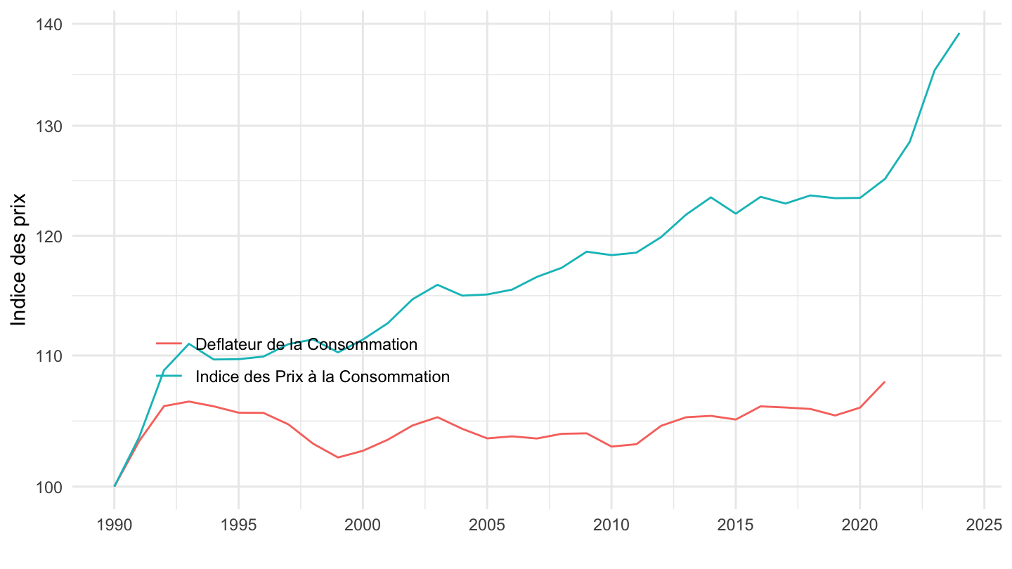
09.4 - Services récréatifs et culturels
Code
`conso-eff-fonction` %>%
  filter(fonction == "09.4",
         variable == "Iprix2014") %>%
  year_to_date2 %>%
  filter(date >= as.Date("1990-01-01")) %>%
  mutate(variable = "Deflateur de la Consommation") %>%
  select(variable, date, value) %>%
  bind_rows(`IPC-2015` %>%
              filter(INDICATEUR == "IPC",
                     MENAGES_IPC == "ENSEMBLE",
                     COICOP2016 %in% c("094"),
                     FREQ == "M",
                     REF_AREA == "FE",
                     NATURE == "INDICE") %>%
              month_to_date %>%
              filter(month(date) == 1) %>%
              select(date, value = OBS_VALUE) %>%
              mutate(variable = "Indice des Prix à la Consommation")) %>%
  group_by(variable) %>%
  mutate(value = 100*value/value[date == as.Date("1990-01-01")]) %>%
  ggplot() + ylab("Indice des prix") + xlab("") + theme_minimal() +
  geom_line(aes(x = date, y = value, color = variable)) +

  scale_x_date(breaks = seq(1920, 2025, 5) %>% paste0("-01-01") %>% as.Date,
               labels = date_format("%Y")) +
  theme(legend.position = c(0.25, 0.3),
        legend.title = element_blank()) +
  scale_y_log10(breaks = c(seq(0, 500, 10), 15),
                     labels = dollar_format(accuracy = 1, prefix = ""))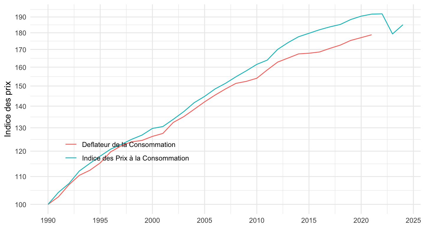
09.5 - Journaux, livres et articles de papeterie
Code
`conso-eff-fonction` %>%
  filter(fonction == "09.5",
         variable == "Iprix2014") %>%
  year_to_date2 %>%
  filter(date >= as.Date("1990-01-01")) %>%
  mutate(variable = "Deflateur de la Consommation") %>%
  select(variable, date, value) %>%
  bind_rows(`IPC-2015` %>%
              filter(INDICATEUR == "IPC",
                     MENAGES_IPC == "ENSEMBLE",
                     COICOP2016 %in% c("095"),
                     FREQ == "M",
                     REF_AREA == "FE",
                     NATURE == "INDICE") %>%
              month_to_date %>%
              filter(month(date) == 1) %>%
              select(date, value = OBS_VALUE) %>%
              mutate(variable = "Indice des Prix à la Consommation")) %>%
  group_by(variable) %>%
  mutate(value = 100*value/value[date == as.Date("1990-01-01")]) %>%
  ggplot() + ylab("Indice des prix") + xlab("") + theme_minimal() +
  geom_line(aes(x = date, y = value, color = variable)) +

  scale_x_date(breaks = seq(1920, 2025, 5) %>% paste0("-01-01") %>% as.Date,
               labels = date_format("%Y")) +
  theme(legend.position = c(0.25, 0.8),
        legend.title = element_blank()) +
  scale_y_log10(breaks = c(seq(0, 500, 10), 15),
                     labels = dollar_format(accuracy = 1, prefix = ""))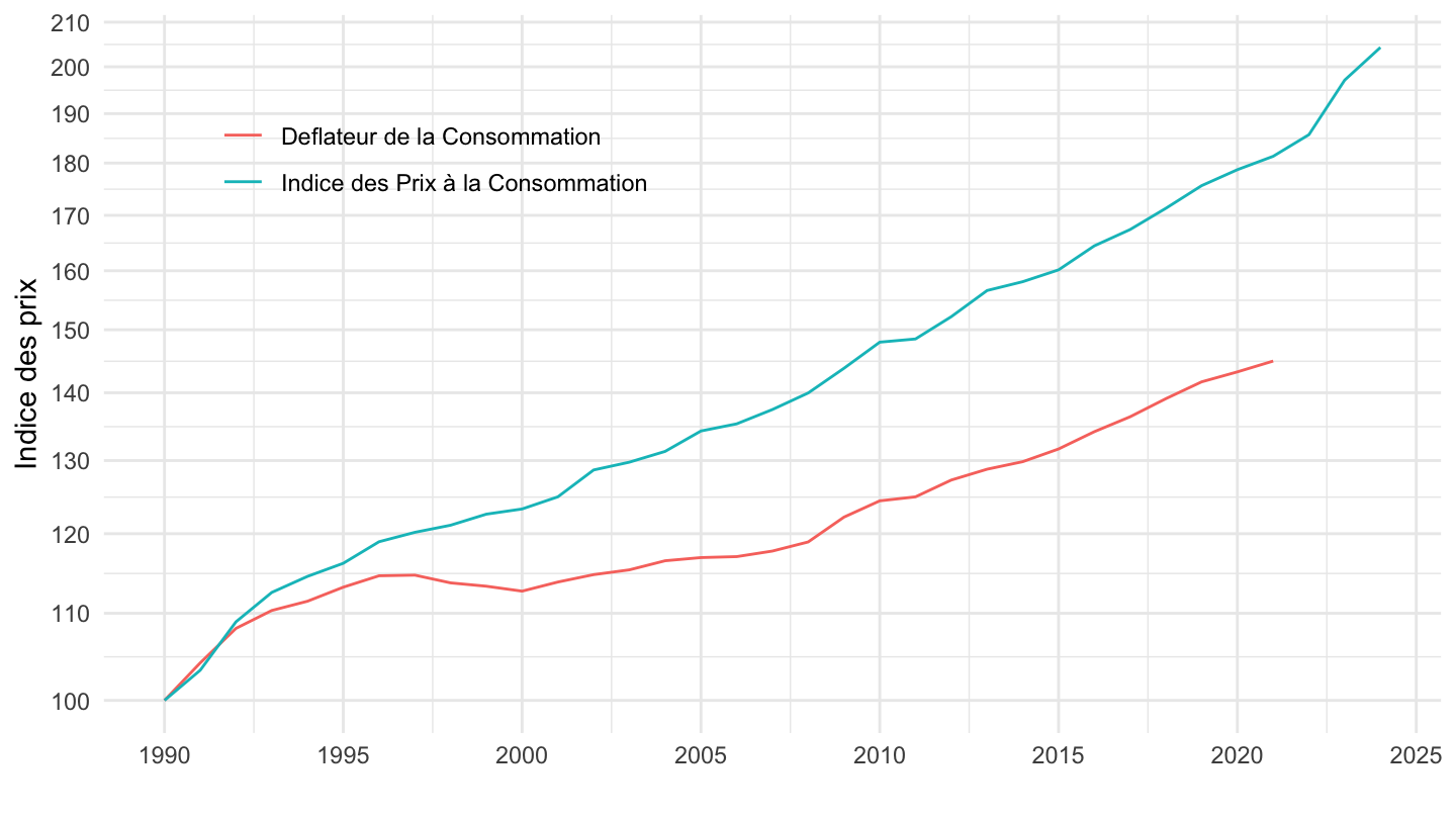
09.6 - Forfaits touristiques
Code
`conso-eff-fonction` %>%
  filter(fonction == "09.6",
         variable == "Iprix2014") %>%
  year_to_date2 %>%
  filter(date >= as.Date("1990-01-01")) %>%
  mutate(variable = "Deflateur de la Consommation") %>%
  select(variable, date, value) %>%
  bind_rows(`IPC-2015` %>%
              filter(INDICATEUR == "IPC",
                     MENAGES_IPC == "ENSEMBLE",
                     COICOP2016 %in% c("096"),
                     FREQ == "M",
                     REF_AREA == "FE",
                     NATURE == "INDICE") %>%
              month_to_date %>%
              filter(month(date) == 1) %>%
              select(date, value = OBS_VALUE) %>%
              mutate(variable = "Indice des Prix à la Consommation")) %>%
  group_by(variable) %>%
  mutate(value = 100*value/value[date == as.Date("1990-01-01")]) %>%
  ggplot() + ylab("Indice des prix") + xlab("") + theme_minimal() +
  geom_line(aes(x = date, y = value, color = variable)) +

  scale_x_date(breaks = seq(1920, 2025, 5) %>% paste0("-01-01") %>% as.Date,
               labels = date_format("%Y")) +
  theme(legend.position = c(0.25, 0.8),
        legend.title = element_blank()) +
  scale_y_log10(breaks = c(seq(0, 500, 10), 15),
                     labels = dollar_format(accuracy = 1, prefix = ""))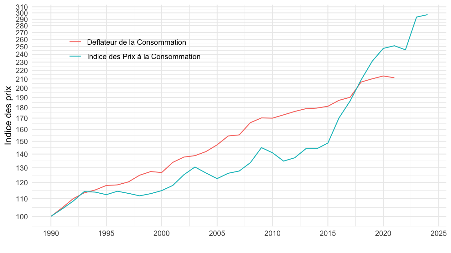
12.6 - Services financiers
Code
`conso-eff-fonction` %>%
  filter(fonction == "12.6",
         variable == "Iprix2014") %>%
  year_to_date2 %>%
  filter(date >= as.Date("1990-01-01")) %>%
  mutate(variable = "Deflateur de la Consommation") %>%
  select(variable, date, value) %>%
  bind_rows(`IPC-2015` %>%
              filter(INDICATEUR == "IPC",
                     MENAGES_IPC == "ENSEMBLE",
                     COICOP2016 %in% c("126"),
                     FREQ == "M",
                     REF_AREA == "FE",
                     NATURE == "INDICE") %>%
              month_to_date %>%
              filter(month(date) == 1) %>%
              select(date, value = OBS_VALUE) %>%
              mutate(variable = "Indice des Prix à la Consommation")) %>%
  group_by(variable) %>%
  mutate(value = 100*value/value[date == as.Date("1990-01-01")]) %>%
  ggplot() + ylab("Indice des prix") + xlab("") + theme_minimal() +
  geom_line(aes(x = date, y = value, color = variable)) +

  scale_x_date(breaks = seq(1920, 2025, 5) %>% paste0("-01-01") %>% as.Date,
               labels = date_format("%Y")) +
  theme(legend.position = c(0.75, 0.7),
        legend.title = element_blank()) +
  scale_y_log10(breaks = seq(0, 500, 10),
                     labels = dollar_format(accuracy = 1, prefix = ""))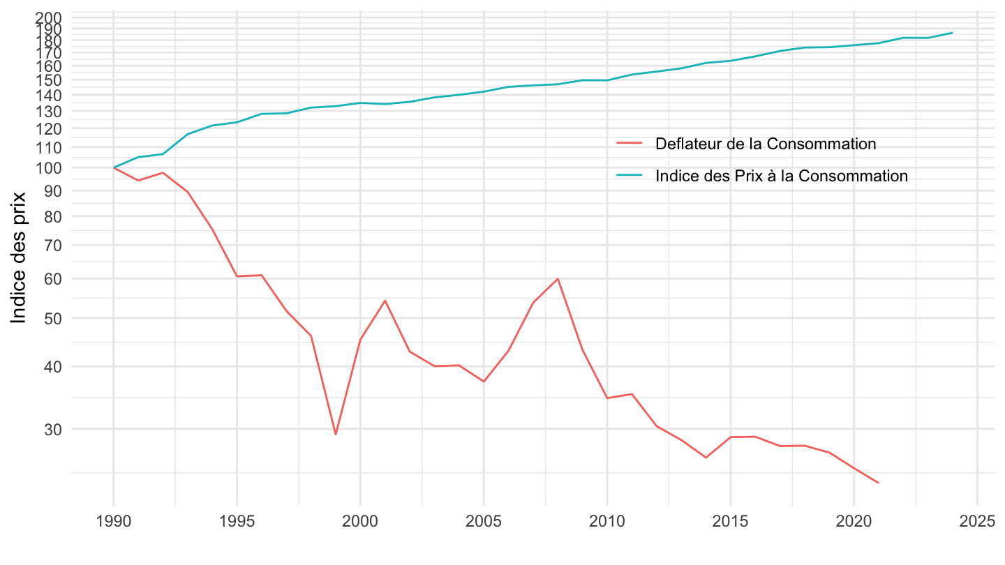
14.1 - Logement
Code
`conso-eff-fonction` %>%
  filter(fonction == "14.1",
         variable == "Iprix2014") %>%
  year_to_date2 %>%
  filter(date >= as.Date("1990-01-01")) %>%
  mutate(variable = "Deflateur de la Consommation") %>%
  select(variable, date, value) %>%
  group_by(variable) %>%
  mutate(value = 100*value/value[date == as.Date("1990-01-01")]) %>%
  ggplot() + ylab("Indice des prix") + xlab("") + theme_minimal() +
  geom_line(aes(x = date, y = value, color = variable)) +

  scale_x_date(breaks = seq(1920, 2025, 5) %>% paste0("-01-01") %>% as.Date,
               labels = date_format("%Y")) +
  theme(legend.position = c(0.25, 0.9),
        legend.title = element_blank()) +
  scale_y_log10(breaks = seq(0, 500, 10),
                     labels = dollar_format(accuracy = 1, prefix = ""))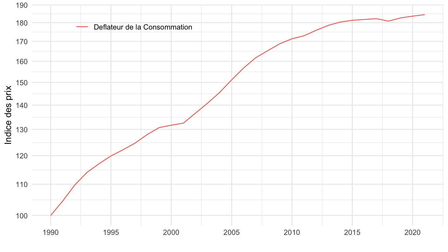
14.2 - Santé
Code
`conso-eff-fonction` %>%
  filter(fonction == "14.2",
         variable == "Iprix2014") %>%
  year_to_date2 %>%
  filter(date >= as.Date("1990-01-01")) %>%
  mutate(variable = "Deflateur de la Consommation") %>%
  select(variable, date, value) %>%
  group_by(variable) %>%
  mutate(value = 100*value/value[date == as.Date("1990-01-01")]) %>%
  ggplot() + ylab("Indice des prix") + xlab("") + theme_minimal() +
  geom_line(aes(x = date, y = value, color = variable)) +

  scale_x_date(breaks = seq(1920, 2025, 5) %>% paste0("-01-01") %>% as.Date,
               labels = date_format("%Y")) +
  theme(legend.position = c(0.25, 0.9),
        legend.title = element_blank()) +
  scale_y_log10(breaks = seq(0, 500, 10),
                     labels = dollar_format(accuracy = 1, prefix = ""))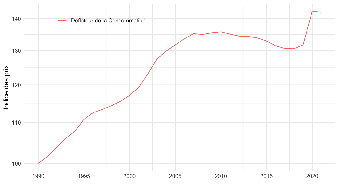
14.3 - Loisirs et culture
Code
`conso-eff-fonction` %>%
  filter(fonction == "14.3",
         variable == "Iprix2014") %>%
  year_to_date2 %>%
  filter(date >= as.Date("1990-01-01")) %>%
  mutate(variable = "Deflateur de la Consommation") %>%
  select(variable, date, value) %>%
  group_by(variable) %>%
  mutate(value = 100*value/value[date == as.Date("1990-01-01")]) %>%
  ggplot() + ylab("Indice des prix") + xlab("") + theme_minimal() +
  geom_line(aes(x = date, y = value, color = variable)) +

  scale_x_date(breaks = seq(1920, 2025, 5) %>% paste0("-01-01") %>% as.Date,
               labels = date_format("%Y")) +
  theme(legend.position = c(0.25, 0.9),
        legend.title = element_blank()) +
  scale_y_log10(breaks = seq(0, 500, 10),
                     labels = dollar_format(accuracy = 1, prefix = ""))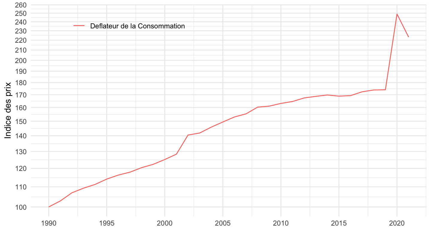
14.4 - Enseignement
Code
`conso-eff-fonction` %>%
  filter(fonction == "14.4",
         variable == "Iprix2014") %>%
  year_to_date2 %>%
  filter(date >= as.Date("1990-01-01")) %>%
  mutate(variable = "Deflateur de la Consommation") %>%
  select(variable, date, value) %>%
  group_by(variable) %>%
  mutate(value = 100*value/value[date == as.Date("1990-01-01")]) %>%
  ggplot() + ylab("Indice des prix") + xlab("") + theme_minimal() +
  geom_line(aes(x = date, y = value, color = variable)) +

  scale_x_date(breaks = seq(1920, 2025, 5) %>% paste0("-01-01") %>% as.Date,
               labels = date_format("%Y")) +
  theme(legend.position = c(0.25, 0.9),
        legend.title = element_blank()) +
  scale_y_log10(breaks = seq(0, 500, 10),
                     labels = dollar_format(accuracy = 1, prefix = ""))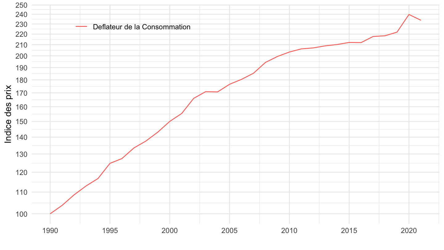
4-digit
05.6.2 - Services domestiques et services ménagers
Code
`conso-eff-fonction` %>%
  filter(fonction == "05.6.2",
         variable == "Iprix2014") %>%
  year_to_date2 %>%
  filter(date >= as.Date("1990-01-01")) %>%
  mutate(variable = "Deflateur de la Consommation") %>%
  select(variable, date, value) %>%
  bind_rows(`IPC-2015` %>%
              filter(INDICATEUR == "IPC",
                     MENAGES_IPC == "ENSEMBLE",
                     COICOP2016 %in% c("0562"),
                     FREQ == "M",
                     REF_AREA == "FE",
                     NATURE == "INDICE") %>%
              month_to_date %>%
              filter(month(date) == 1) %>%
              select(date, value = OBS_VALUE) %>%
              mutate(variable = "Indice des Prix à la Consommation")) %>%
  group_by(variable) %>%
  mutate(value = 100*value/value[date == as.Date("1990-01-01")]) %>%
  ggplot() + ylab("Indice des prix") + xlab("") + theme_minimal() +
  geom_line(aes(x = date, y = value, color = variable)) +

  scale_x_date(breaks = seq(1920, 2025, 5) %>% paste0("-01-01") %>% as.Date,
               labels = date_format("%Y")) +
  theme(legend.position = c(0.25, 0.9),
        legend.title = element_blank()) +
  scale_y_log10(breaks = seq(0, 500, 10),
                     labels = dollar_format(accuracy = 1, prefix = ""))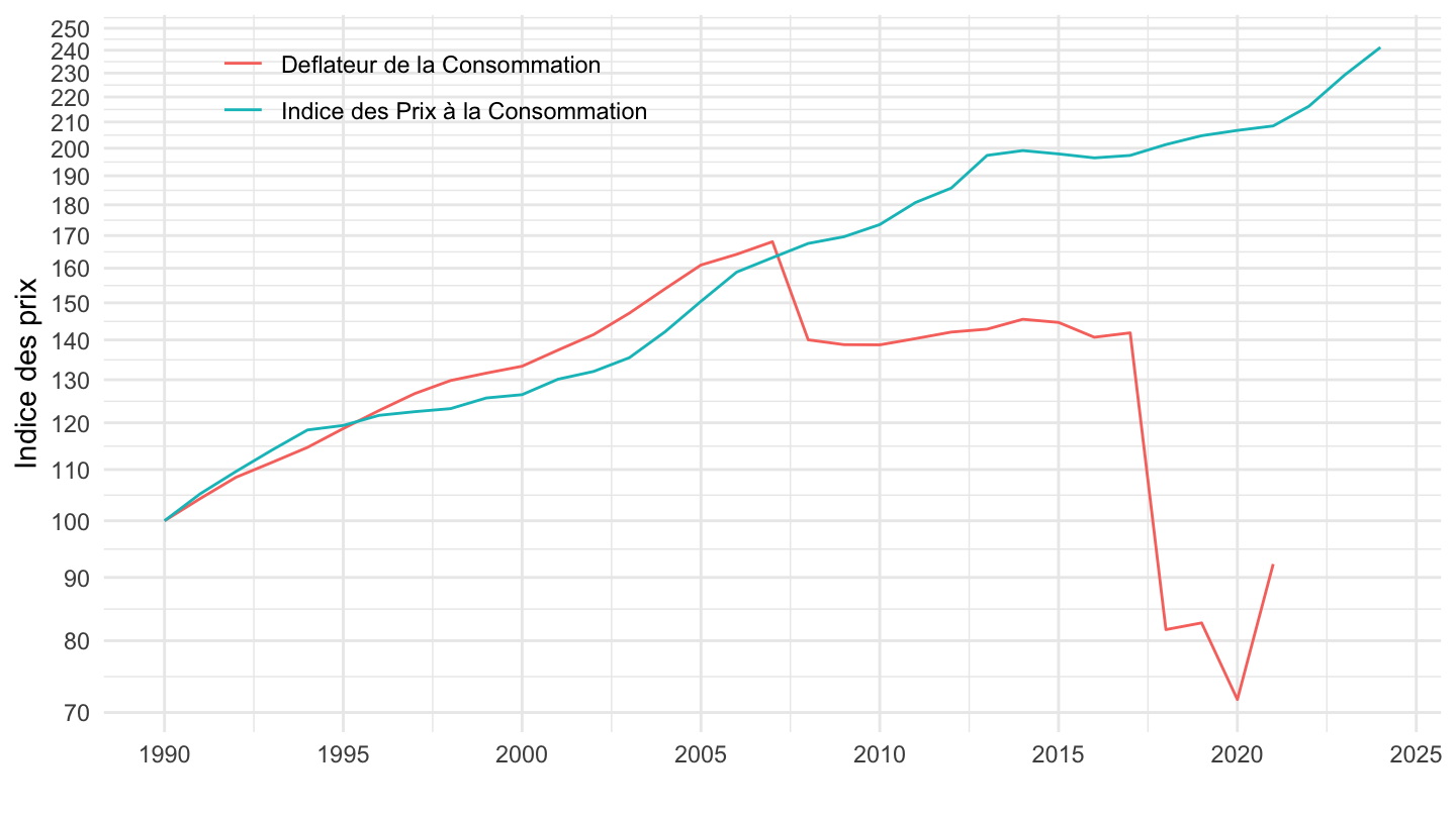
09.1.1 -
Code
`conso-eff-fonction` %>%
  filter(fonction == "09.1.2",
         variable == "Iprix2014") %>%
  year_to_date2 %>%
  filter(date >= as.Date("1990-01-01")) %>%
  mutate(variable = "Deflateur de la Consommation") %>%
  select(variable, date, value) %>%
  bind_rows(`IPC-2015` %>%
              filter(INDICATEUR == "IPC",
                     MENAGES_IPC == "ENSEMBLE",
                     COICOP2016 %in% c("0912"),
                     FREQ == "M",
                     REF_AREA == "FE",
                     NATURE == "INDICE") %>%
              month_to_date %>%
              filter(month(date) == 1) %>%
              select(date, value = OBS_VALUE) %>%
              mutate(variable = "Indice des Prix à la Consommation")) %>%
  group_by(variable) %>%
  mutate(value = 100*value/value[date == as.Date("1990-01-01")]) %>%
  ggplot() + ylab("Indice des prix") + xlab("") + theme_minimal() +
  geom_line(aes(x = date, y = value, color = variable)) +

  scale_x_date(breaks = seq(1920, 2025, 5) %>% paste0("-01-01") %>% as.Date,
               labels = date_format("%Y")) +
  theme(legend.position = c(0.75, 0.3),
        legend.title = element_blank()) +
  scale_y_log10(breaks = seq(0, 500, 10),
                     labels = dollar_format(accuracy = 1, prefix = ""))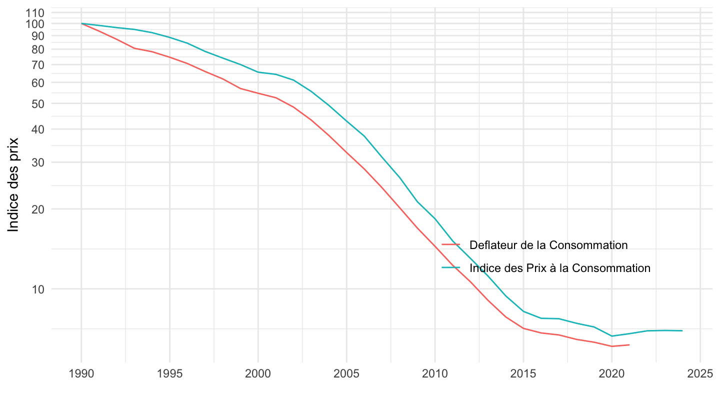
09.1.4
Code
`conso-eff-fonction` %>%
  filter(fonction == "09.1.4",
         variable == "Iprix2014") %>%
  year_to_date2 %>%
  filter(date >= as.Date("1990-01-01")) %>%
  mutate(variable = "Deflateur de la Consommation") %>%
  select(variable, date, value) %>%
  bind_rows(`IPC-2015` %>%
              filter(INDICATEUR == "IPC",
                     MENAGES_IPC == "ENSEMBLE",
                     COICOP2016 %in% c("0914"),
                     FREQ == "M",
                     REF_AREA == "FE",
                     NATURE == "INDICE") %>%
              month_to_date %>%
              filter(month(date) == 1) %>%
              select(date, value = OBS_VALUE) %>%
              mutate(variable = "Indice des Prix à la Consommation")) %>%
  group_by(variable) %>%
  mutate(value = 100*value/value[date == as.Date("1990-01-01")]) %>%
  ggplot() + ylab("Indice des prix") + xlab("") + theme_minimal() +
  geom_line(aes(x = date, y = value, color = variable)) +

  scale_x_date(breaks = seq(1920, 2025, 5) %>% paste0("-01-01") %>% as.Date,
               labels = date_format("%Y")) +
  theme(legend.position = c(0.75, 0.3),
        legend.title = element_blank()) +
  scale_y_log10(breaks = seq(0, 500, 10),
                     labels = dollar_format(accuracy = 1, prefix = ""))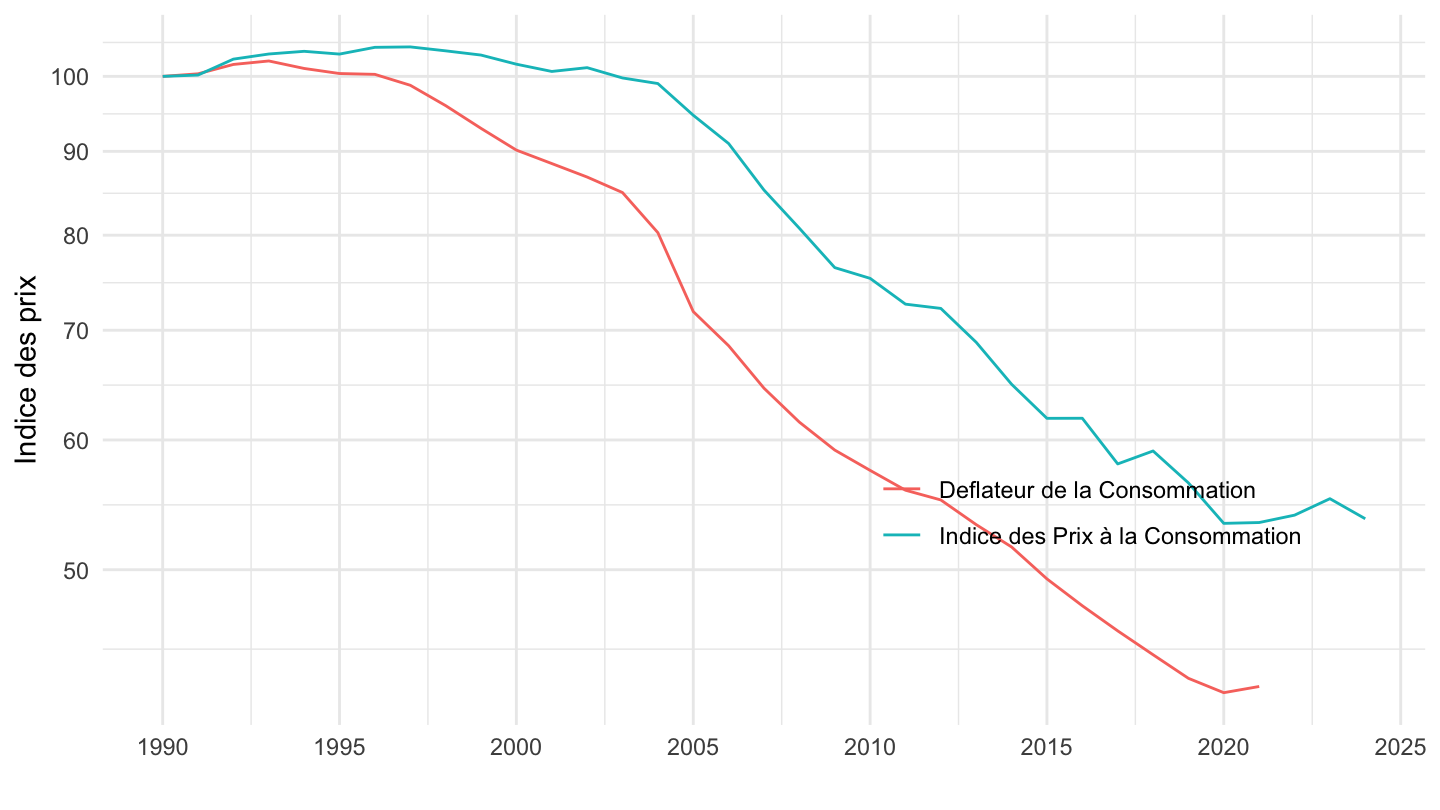
09.1.5 - Réparation de matériels audiovisuel, photographique et informatique
Code
`conso-eff-fonction` %>%
  filter(fonction == "09.1.5",
         variable == "Iprix2014") %>%
  year_to_date2 %>%
  filter(date >= as.Date("1990-01-01")) %>%
  mutate(variable = "Deflateur de la Consommation") %>%
  select(variable, date, value) %>%
  bind_rows(`IPC-2015` %>%
              filter(INDICATEUR == "IPC",
                     MENAGES_IPC == "ENSEMBLE",
                     COICOP2016 %in% c("0914"),
                     FREQ == "M",
                     REF_AREA == "FE",
                     NATURE == "INDICE") %>%
              month_to_date %>%
              filter(month(date) == 1) %>%
              select(date, value = OBS_VALUE) %>%
              mutate(variable = "Indice des Prix à la Consommation")) %>%
  group_by(variable) %>%
  mutate(value = 100*value/value[date == as.Date("1990-01-01")]) %>%
  ggplot() + ylab("Indice des prix") + xlab("") + theme_minimal() +
  geom_line(aes(x = date, y = value, color = variable)) +

  scale_x_date(breaks = seq(1920, 2025, 5) %>% paste0("-01-01") %>% as.Date,
               labels = date_format("%Y")) +
  theme(legend.position = c(0.75, 0.3),
        legend.title = element_blank()) +
  scale_y_log10(breaks = seq(0, 500, 10),
                     labels = dollar_format(accuracy = 1, prefix = ""))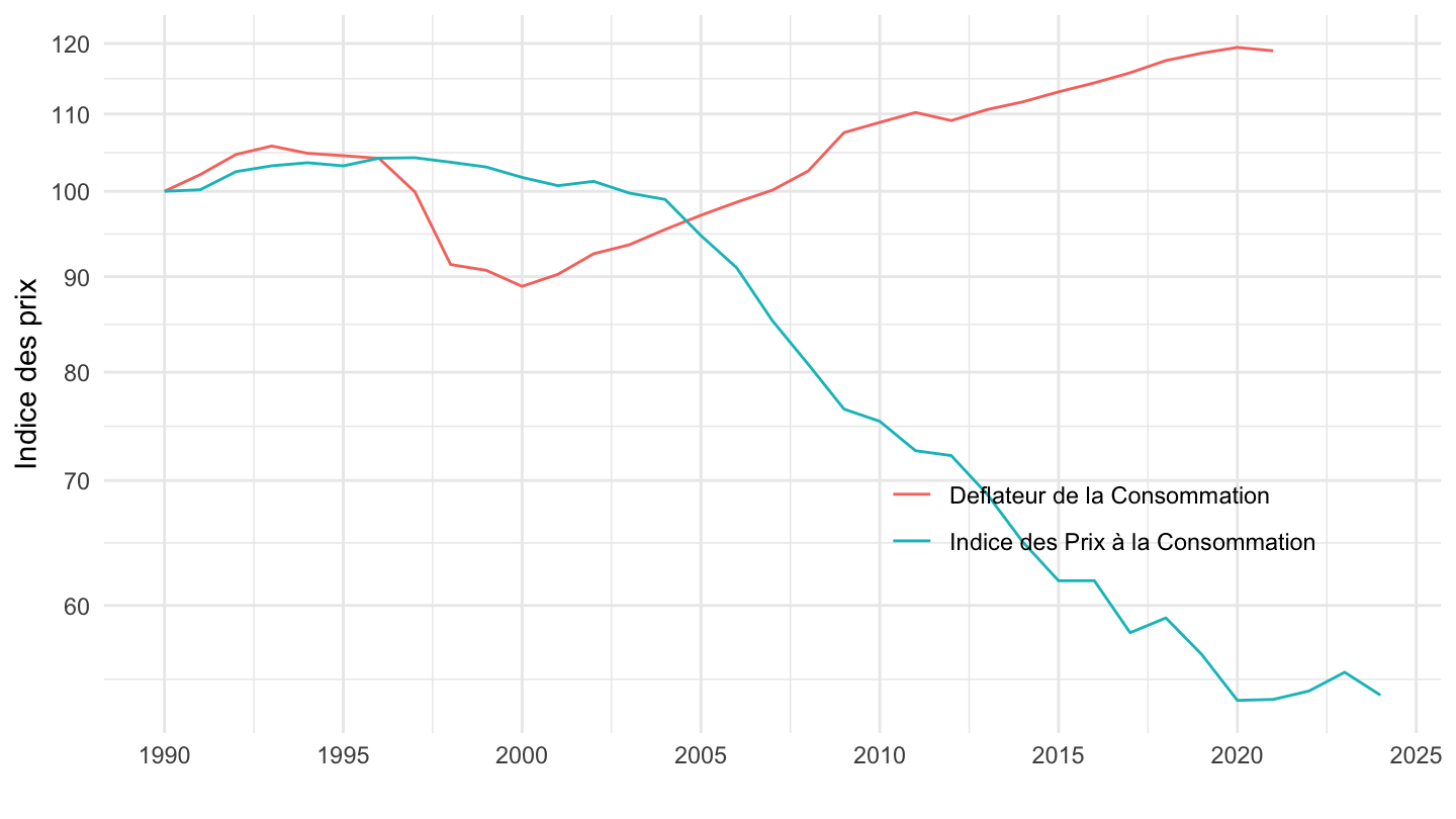
09.3.1 - Jeux, jouets et passe-temps
Code
`conso-eff-fonction` %>%
  filter(fonction == "09.3.1",
         variable == "Iprix2014") %>%
  year_to_date2 %>%
  filter(date >= as.Date("1990-01-01")) %>%
  mutate(variable = "Deflateur de la Consommation") %>%
  select(variable, date, value) %>%
  bind_rows(`IPC-2015` %>%
              filter(INDICATEUR == "IPC",
                     MENAGES_IPC == "ENSEMBLE",
                     COICOP2016 %in% c("0931"),
                     FREQ == "M",
                     REF_AREA == "FE",
                     NATURE == "INDICE") %>%
              month_to_date %>%
              filter(month(date) == 1) %>%
              select(date, value = OBS_VALUE) %>%
              mutate(variable = "Indice des Prix à la Consommation")) %>%
  group_by(variable) %>%
  mutate(value = 100*value/value[date == as.Date("1990-01-01")]) %>%
  ggplot() + ylab("Indice des prix") + xlab("") + theme_minimal() +
  geom_line(aes(x = date, y = value, color = variable)) +

  scale_x_date(breaks = seq(1920, 2025, 5) %>% paste0("-01-01") %>% as.Date,
               labels = date_format("%Y")) +
  theme(legend.position = c(0.25, 0.9),
        legend.title = element_blank()) +
  scale_y_log10(breaks = seq(0, 500, 10),
                     labels = dollar_format(accuracy = 1, prefix = ""))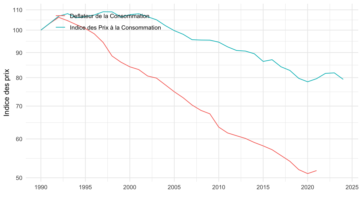
09.5.4 - Papeterie et matériel de dessin
Code
`conso-eff-fonction` %>%
  filter(fonction == "09.5.4",
         variable == "Iprix2014") %>%
  year_to_date2 %>%
  filter(date >= as.Date("1990-01-01")) %>%
  mutate(variable = "Deflateur de la Consommation") %>%
  select(variable, date, value) %>%
  bind_rows(`IPC-2015` %>%
              filter(INDICATEUR == "IPC",
                     MENAGES_IPC == "ENSEMBLE",
                     COICOP2016 %in% c("0954"),
                     FREQ == "M",
                     REF_AREA == "FE",
                     NATURE == "INDICE") %>%
              month_to_date %>%
              filter(month(date) == 1) %>%
              select(date, value = OBS_VALUE) %>%
              mutate(variable = "Indice des Prix à la Consommation")) %>%
  group_by(variable) %>%
  mutate(value = 100*value/value[date == as.Date("1990-01-01")]) %>%
  ggplot() + ylab("Indice des prix") + xlab("") + theme_minimal() +
  geom_line(aes(x = date, y = value, color = variable)) +

  scale_x_date(breaks = seq(1920, 2025, 5) %>% paste0("-01-01") %>% as.Date,
               labels = date_format("%Y")) +
  theme(legend.position = c(0.25, 0.9),
        legend.title = element_blank()) +
  scale_y_log10(breaks = seq(0, 500, 10),
                     labels = dollar_format(accuracy = 1, prefix = ""))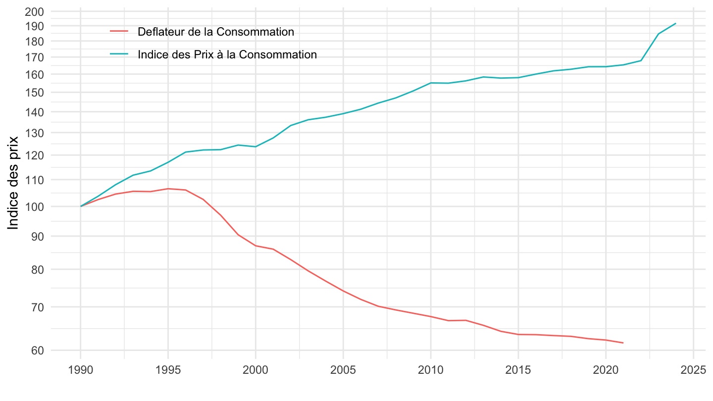
12.6.1 - Services financiers indirectement mesurés
Code
`conso-eff-fonction` %>%
  filter(fonction == "12.6.1",
         variable == "Iprix2014") %>%
  year_to_date2 %>%
  filter(date >= as.Date("1990-01-01")) %>%
  mutate(variable = "Deflateur de la Consommation") %>%
  select(variable, date, value) %>%
  group_by(variable) %>%
  mutate(value = 100*value/value[date == as.Date("1990-01-01")]) %>%
  ggplot() + ylab("Indice des prix") + xlab("") + theme_minimal() +
  geom_line(aes(x = date, y = value, color = variable)) +

  scale_x_date(breaks = seq(1920, 2025, 5) %>% paste0("-01-01") %>% as.Date,
               labels = date_format("%Y")) +
  theme(legend.position = c(0.75, 0.7),
        legend.title = element_blank()) +
  scale_y_log10(breaks = seq(0, 500, 10),
                     labels = dollar_format(accuracy = 1, prefix = ""))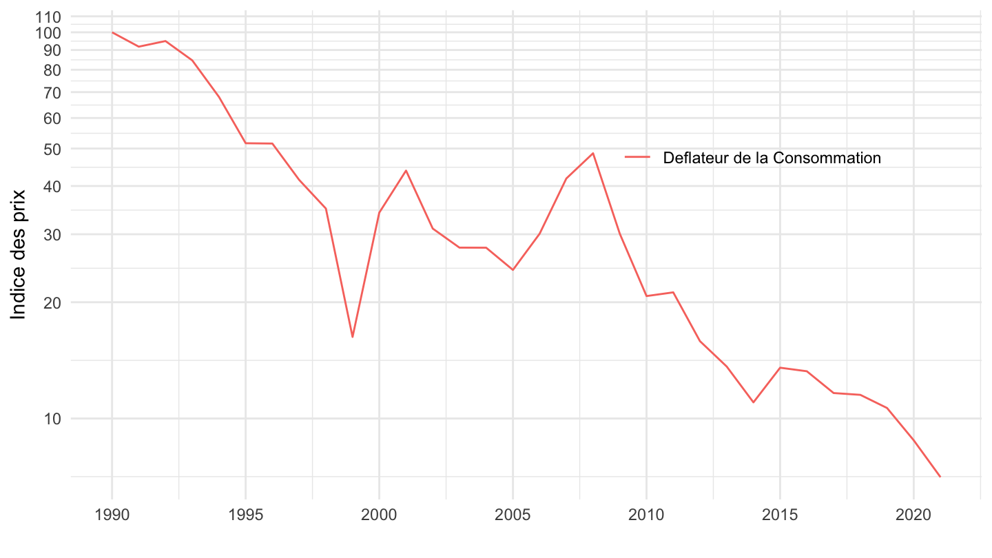
Différences
- Santé est en categorie 13 et 14 dans la COICOP lorsque c’est une dépense de consommation des APU ou des IBSLM, ie dans le déflateur de la consommation finale (pareil dans l’IPCH). Dans l’IPC en revanche, la santé est incluse dans la classification n°6 ce qui apparait contradictoire…