| source | dataset | Title | .html | .rData |
|---|---|---|---|---|
| insee | t_pouvachat_val | Pouvoir d'achat et ratios des comptes des ménages | 2026-07-23 | 2026-02-27 |
Pouvoir d’achat et ratios des comptes des ménages
Données - INSEE
Info
Données
Données sur le pouvoir d’achat
| source | dataset | Title | .html | .rData |
|---|---|---|---|---|
| insee | CNA-2014-RDB | Revenu et pouvoir d’achat des ménages | 2026-07-23 | 2026-07-23 |
| insee | CNT-2014-CSI | Comptes de secteurs institutionnels | 2026-07-23 | 2026-07-22 |
| insee | T_2101 | 2.101 – Revenu disponible brut des ménages et évolution du pouvoir d'achat par personne, par ménage et par unité de consommation (En milliards euros et %) | 2026-07-23 | 2025-12-14 |
| insee | T_7401 | 7.401 – Compte des ménages (S14) (En milliards d'euros) | 2026-07-23 | 2025-12-14 |
| insee | conso-eff-fonction | Consommation effective des ménages par fonction | 2026-07-23 | 2022-06-14 |
| insee | econ-gen-revenu-dispo-pouv-achat-2 | Revenu disponible brut et pouvoir d’achat - Données annuelles | 2026-07-23 | 2026-01-11 |
| insee | reve-conso-evo-dep-pa | Évolution de la dépense et du pouvoir d’achat des ménages - Données annuelles de 1960 à 2023 | 2026-07-23 | 2024-12-11 |
| insee | reve-niv-vie-individu-activite | Niveau de vie selon l'activité - Données annuelles | 2026-07-23 | 2025-12-22 |
| insee | reve-niv-vie-pouv-achat-trim | Évolution du revenu disponible brut et du pouvoir d’achat - Données trimestrielles | 2026-07-23 | 2026-01-11 |
| insee | t_men_val | Revenu, pouvoir d'achat et comptes des ménages - Valeurs aux prix courants | 2026-07-23 | 2026-02-27 |
| insee | t_pouvachat_val | Pouvoir d'achat et ratios des comptes des ménages | 2026-07-23 | 2026-02-27 |
| insee | t_recapAgent_val | Récapitulatif des séries des comptes d'agents | 2026-07-23 | 2026-02-27 |
| insee | t_salaire_val | Salaire moyen par tête - SMPT (données CVS) | 2026-07-23 | 2026-02-27 |
| oecd | HH_DASH | Household Dashboard | 2026-07-23 | 2023-09-09 |
Bibliographie en lien
Français
« Mesurer “le” pouvoir d’achat », F. Geerolf, 9 juillet 2024. [ html] [ pdf] [ handouts] [ slides] [ slides] [ github]
« La taxe inflationniste, le pouvoir d’achat, le taux d’épargne et le déficit public », F. Geerolf, 9 juillet 2024. [ html] [ pdf] [ handouts] [ slides] [ slides] [ github]
« Inflation en France : IPC ou IPCH ? », F. Geerolf, 9 juillet 2024. [ html] [ pdf] [ handouts] [ slides] [ slides] [ github]
Données sur l’épargne
| source | dataset | Title | .html | .rData |
|---|---|---|---|---|
| bdf | CFT | Comptes Financiers Trimestriels | 2026-07-23 | 2025-03-09 |
| insee | T_7401 | 7.401 – Compte des ménages (S14) (En milliards d'euros) | 2026-07-23 | 2025-12-14 |
| insee | bdf2017 | Budget de famille 2017 | 2026-07-23 | 2023-11-21 |
| insee | ip1815 | Plus d’épargne chez les plus aisés, plus de dépenses contraintes chez les plus modestes - ip1815 | 2026-07-23 | 2023-10-05 |
| insee | t_men_val | Revenu, pouvoir d'achat et comptes des ménages - Valeurs aux prix courants | 2026-07-23 | 2026-02-27 |
| insee | t_pouvachat_val | Pouvoir d'achat et ratios des comptes des ménages | 2026-07-23 | 2026-02-27 |
| insee | t_recapAgent_val | Récapitulatif des séries des comptes d'agents | 2026-07-23 | 2026-02-27 |
LAST_COMPILE
| LAST_COMPILE |
|---|
| 2026-07-24 |
date
Code
t_pouvachat_val %>%
  group_by(date) %>%
  summarise(Nobs = n()) %>%
  arrange(desc(date)) %>%
  print_table_conditional
variable
Code
t_pouvachat_val %>%
  left_join(variable, by = "variable") %>%
  group_by(variable, Variable) %>%
  summarise(Nobs = n()) %>%
print_table_conditional(.)| variable | Variable | Nobs |
|---|---|---|
| (B6/P3prix)/UC | Pouvoir d'achat du RDB par unité de consommation | 307 |
| (B7/P4prix)/UC | Pouvoir d'achat du RDB ajusté par unité de consommation | 307 |
| B6 | RDB | 307 |
| B6 / P3prix | Pouvoir d'achat du RDB | 307 |
| B6/UC | RDB par unité de consommation (UC) | 307 |
| B7 | RDB ajusté | 307 |
| B7/P4prix | Pouvoir d'achat du RDB ajusté | 307 |
| B7/UC | RDB ajusté par unité de consommation | 307 |
| B8/(B6+D8) | Taux d'épargne | 307 |
| B9NF | Épargne financière | 307 |
| B9NF/(B6+D8) | Taux d'épargne financière | 307 |
| P3prix | Prix de la dépense de consommation finale | 307 |
| P3prixhsifim | NA | 191 |
2017T2-
Table
Code
t_pouvachat_val %>%
  left_join(variable, by = "variable") %>%
  filter(date %in% c(as.Date("2017-04-01"), max(date))) %>%
  spread(date, value) %>%
print_table_conditional(.)| variable | Variable | 2017-04-01 | 2025-10-01 |
|---|---|---|---|
| (B6/P3prix)/UC | Pouvoir d'achat du RDB par unité de consommation | 0.4752202 | -0.2926808 |
| (B7/P4prix)/UC | Pouvoir d'achat du RDB ajusté par unité de consommation | 0.4233737 | -0.2172706 |
| B6 | RDB | 0.6476436 | 0.0424540 |
| B6 / P3prix | Pouvoir d'achat du RDB | 0.6158825 | -0.1779846 |
| B6/UC | RDB par unité de consommation (UC) | 0.5069368 | -0.0724954 |
| B7 | RDB ajusté | 0.6862051 | 0.1109755 |
| B7/P4prix | Pouvoir d'achat du RDB ajusté | 0.5639634 | -0.1024877 |
| B7/UC | RDB ajusté par unité de consommation | 0.5454444 | -0.0040527 |
| B8/(B6+D8) | Taux d'épargne | 14.1617062 | 17.8916299 |
| B9NF | Épargne financière | -1.1101410 | -5.9028315 |
| B9NF/(B6+D8) | Taux d'épargne financière | 4.1482424 | 8.5616857 |
| P3prix | Prix de la dépense de consommation finale | 0.0315666 | 0.2208317 |
| P3prixhsifim | NA | 0.0309965 | 0.0521061 |
Pouvoir d’achat du RDB - (B6/P3prix)/UC
Tous
Code
t_pouvachat_val %>%
  filter(variable %in% c("(B6/P3prix)/UC", "B6 / P3prix")) %>%
  left_join(variable, by = "variable") %>%
  group_by(variable, Variable) %>%
  arrange(date) %>%
  mutate(index = c(100, 100*cumprod(1 + value[-1]/100))) %>%
  ggplot() + geom_line(aes(x = date, y = index, color = Variable)) +
  xlab("") + ylab("") + theme_minimal() +
  scale_x_date(breaks = as.Date(paste0(seq(1940, 2100, 5), "-01-01")),
               labels = date_format("%Y")) +
  theme(legend.position = c(0.3, 0.85),
        legend.title = element_blank()) +
  scale_y_log10(breaks = seq(100, 3000, 100))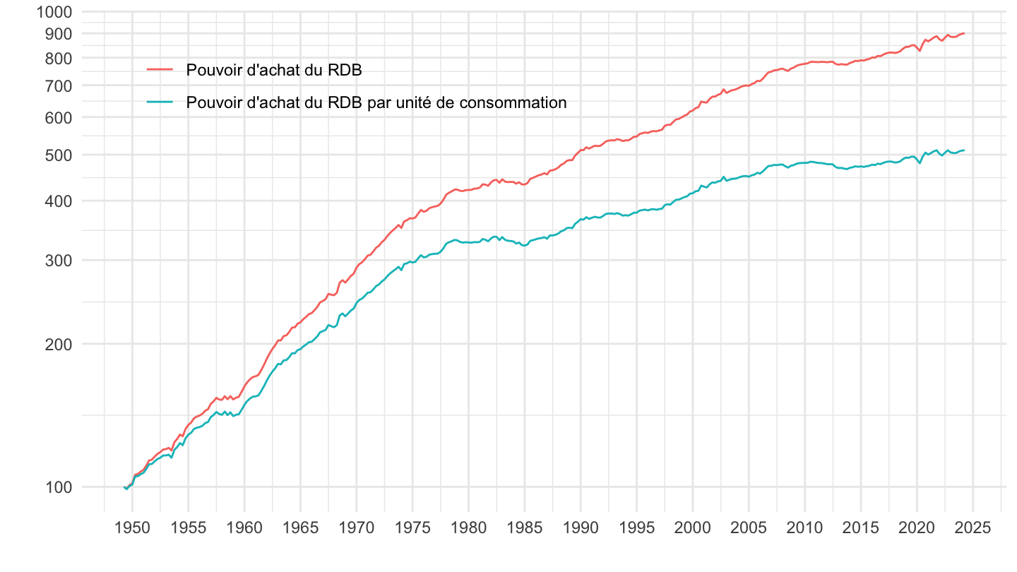
1980-
Code
t_pouvachat_val %>%
  filter(variable %in% c("(B6/P3prix)/UC", "B6 / P3prix")) %>%
  left_join(variable, by = "variable") %>%
  filter(date >= as.Date("1980-01-01")) %>%
  group_by(variable, Variable) %>%
  arrange(date) %>%
  mutate(index = c(100, 100*cumprod(1 + value[-1]/100))) %>%
  ggplot() + geom_line(aes(x = date, y = index, color = Variable)) +
  xlab("") + ylab("") + theme_minimal() +
  scale_x_date(breaks = as.Date(paste0(seq(1980, 2100, 5), "-01-01")),
               labels = date_format("%Y")) +
  theme(legend.position = c(0.3, 0.85),
        legend.title = element_blank()) +
  scale_y_log10(breaks = seq(100, 300, 5))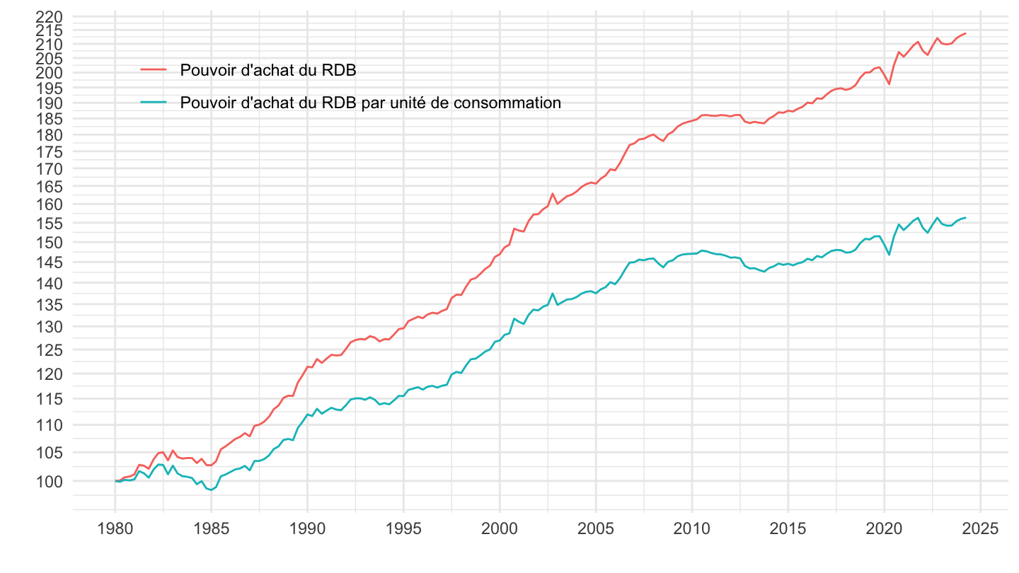
1990-
Code
t_pouvachat_val %>%
  filter(variable %in% c("(B6/P3prix)/UC", "B6 / P3prix")) %>%
  left_join(variable, by = "variable") %>%
  filter(date >= as.Date("1990-01-01")) %>%
  group_by(variable, Variable) %>%
  arrange(date) %>%
  mutate(index = c(100, 100*cumprod(1 + value[-1]/100))) %>%
  ggplot() + geom_line(aes(x = date, y = index, color = Variable)) +
  xlab("") + ylab("") + theme_minimal() +
  scale_x_date(breaks = as.Date(paste0(seq(1990, 2100, 5), "-01-01")),
               labels = date_format("%Y")) +
  theme(legend.position = c(0.3, 0.85),
        legend.title = element_blank()) +
  scale_y_log10(breaks = seq(100, 300, 5))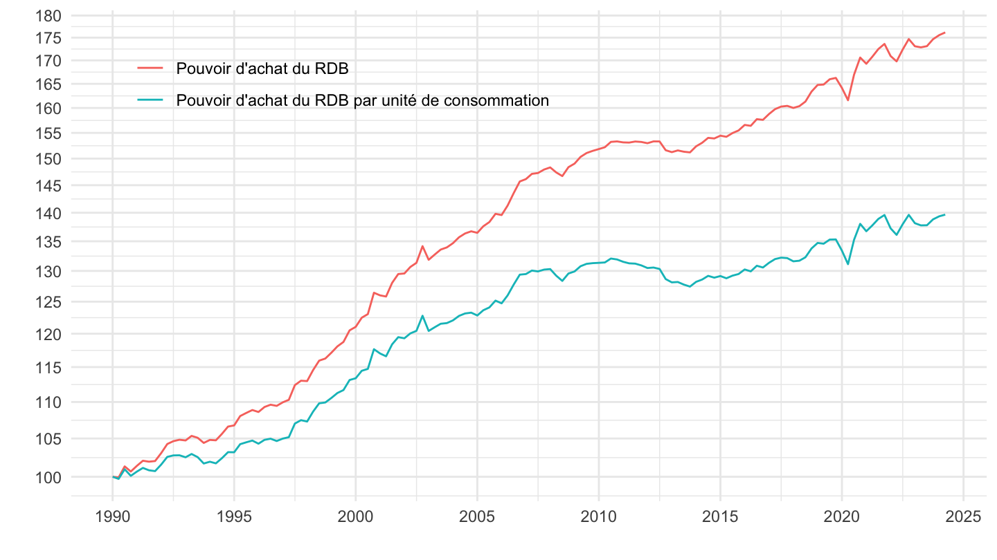
1999-
Code
t_pouvachat_val %>%
  filter(variable %in% c("(B6/P3prix)/UC", "B6 / P3prix")) %>%
  left_join(variable, by = "variable") %>%
  filter(date >= as.Date("1999-01-01")) %>%
  group_by(variable, Variable) %>%
  arrange(date) %>%
  mutate(index = c(100, 100*cumprod(1 + value[-1]/100))) %>%
  ggplot() + geom_line(aes(x = date, y = index, color = Variable)) +
  xlab("") + ylab("") + theme_minimal() +
  scale_x_date(breaks = as.Date(paste0(seq(1999, 2100, 5), "-01-01")),
               labels = date_format("%Y")) +
  theme(legend.position = c(0.3, 0.85),
        legend.title = element_blank()) +
  scale_y_log10(breaks = seq(100, 150, 5))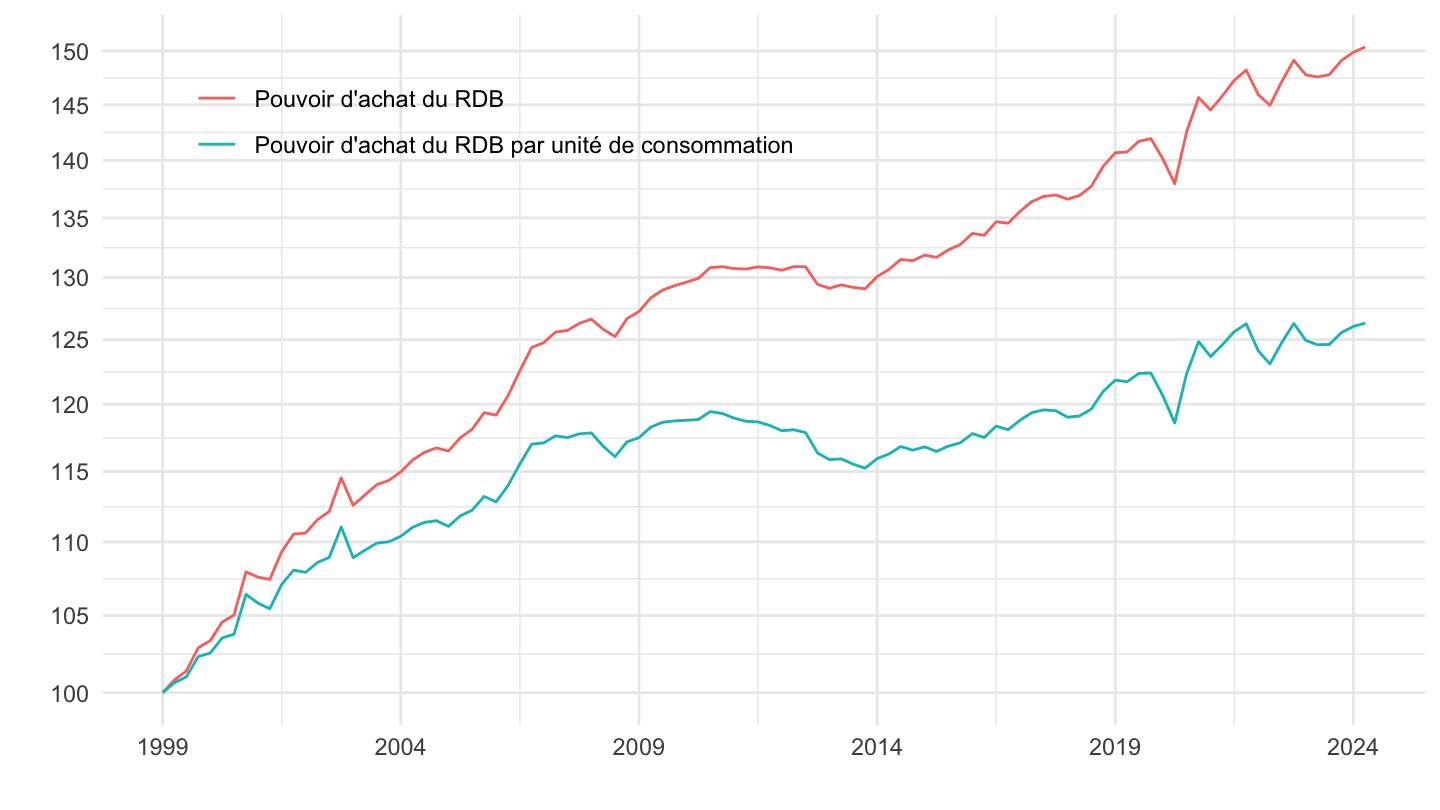
2017T1-
Code
t_pouvachat_val %>%
  filter(variable %in% c("(B6/P3prix)/UC", "B6 / P3prix")) %>%
  left_join(variable, by = "variable") %>%
  filter(date >= as.Date("2017-01-01")) %>%
  group_by(variable, Variable) %>%
  arrange(date) %>%
  mutate(index = c(100, 100*cumprod(1 + value[-1]/100))) %>%
  ggplot() + geom_line(aes(x = date, y = index, color = Variable)) +
  xlab("") + ylab("Indice 100 = 2017T1") + theme_minimal() +
  scale_x_date(breaks = as.Date(paste0(seq(1999, 2100, 1), "-01-01")),
               labels = date_format("%Y")) +
  theme(legend.position = c(0.3, 0.85),
        legend.title = element_blank()) +
  scale_y_log10(breaks = seq(100, 150, 1)) +
  geom_label(data = . %>% filter(date == max(date)),
             aes(x = date, y = index, color = Variable, label = round(index, 1)))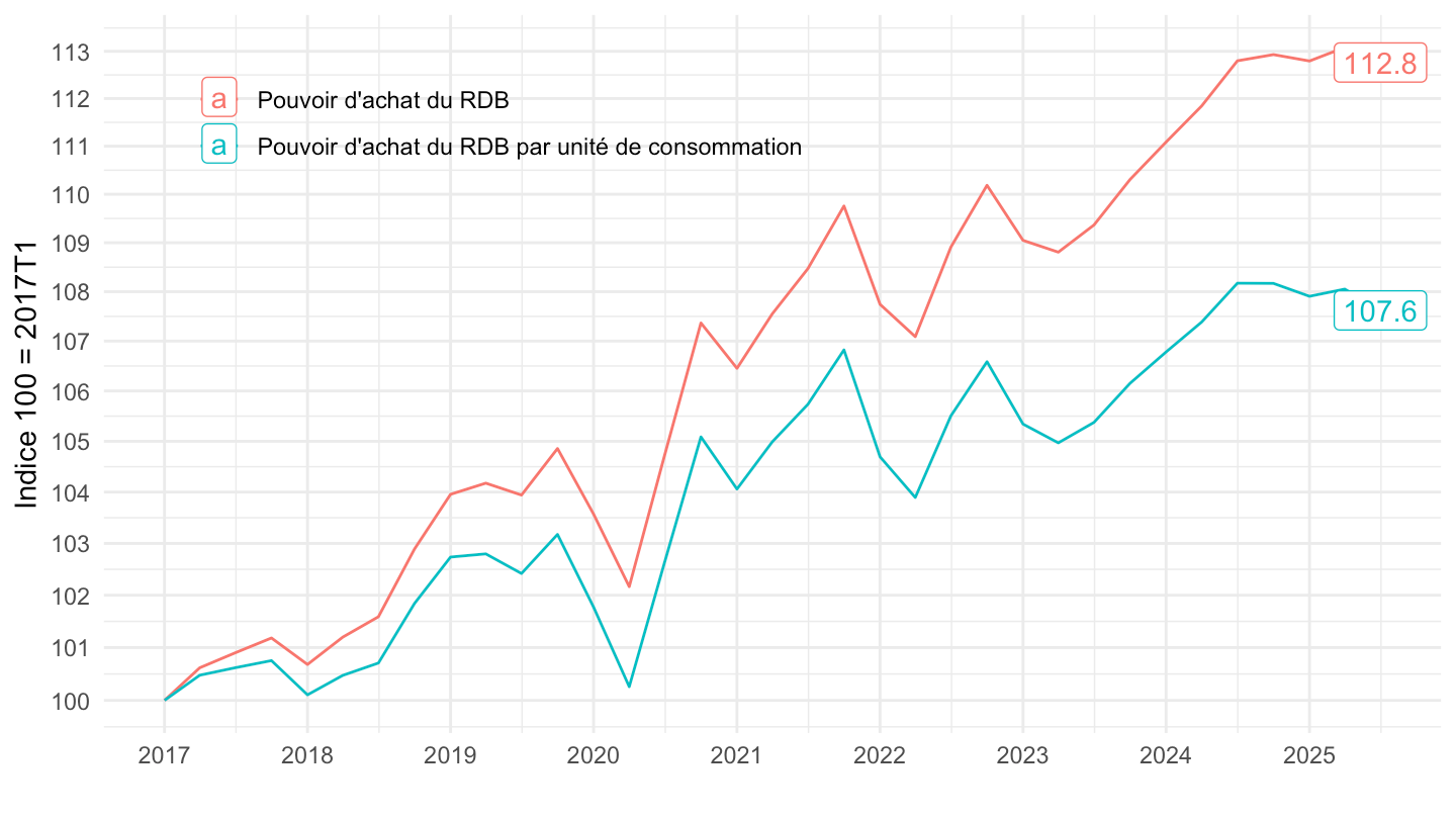
2017T2-
Code
t_pouvachat_val %>%
  filter(variable %in% c("(B6/P3prix)/UC", "B6 / P3prix")) %>%
  left_join(variable, by = "variable") %>%
  filter(date >= as.Date("2017-04-01")) %>%
  group_by(variable, Variable) %>%
  arrange(date) %>%
  mutate(index = c(100, 100*cumprod(1 + value[-1]/100))) %>%
  ggplot() + geom_line(aes(x = date, y = index, color = Variable)) +
  xlab("") + ylab("100 = 2017T2") + theme_minimal() +
  scale_x_date(breaks = as.Date(paste0(seq(1999, 2100, 1), "-01-01")),
               labels = date_format("%Y")) +
  theme(legend.position = c(0.3, 0.85),
        legend.title = element_blank()) +
  scale_y_log10(breaks = seq(100, 150, 1)) +
  geom_label(data = . %>% filter(date == max(date)),
             aes(x = date, y = index, color = Variable, label = round(index, 1)))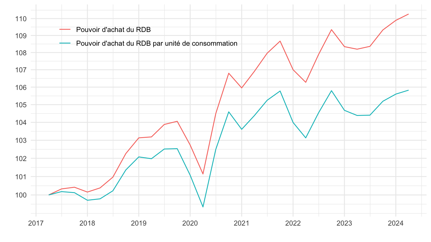
2021T2-
Code
t_pouvachat_val %>%
  filter(variable %in% c("(B6/P3prix)/UC", "B6 / P3prix")) %>%
  left_join(variable, by = "variable") %>%
  filter(date >= as.Date("2021-04-01")) %>%
  group_by(variable, Variable) %>%
  arrange(date) %>%
  mutate(index = c(100, 100*cumprod(1 + value[-1]/100))) %>%
  ggplot() + geom_line(aes(x = date, y = index, color = Variable)) +
  xlab("") + ylab("") + theme_minimal() +
  scale_x_date(breaks = as.Date(paste0(seq(1999, 2100, 1), "-01-01")),
               labels = date_format("%Y")) +
  theme(legend.position = c(0.3, 0.85),
        legend.title = element_blank()) +
  scale_y_log10(breaks = seq(1, 150, 1))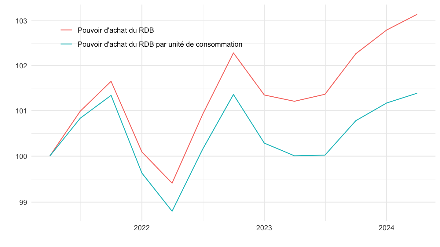
Prix de la dépense de consommation finale - P3prix
Tous
Code
t_pouvachat_val %>%
  filter(variable %in% c("P3prix", "B6", "B7")) %>%
  left_join(variable, by = "variable") %>%
  group_by(variable, Variable) %>%
  arrange(date) %>%
  mutate(index = c(100, 100*cumprod(1 + value[-1]/100))) %>%
  ggplot() + geom_line(aes(x = date, y = index, color = Variable)) +
  xlab("") + ylab("") + theme_minimal() +
  scale_x_date(breaks = as.Date(paste0(seq(1940, 2100, 5), "-01-01")),
               labels = date_format("%Y")) +
  theme(legend.position = c(0.3, 0.85),
        legend.title = element_blank()) +
  scale_y_log10(breaks = seq(100, 100000, 100))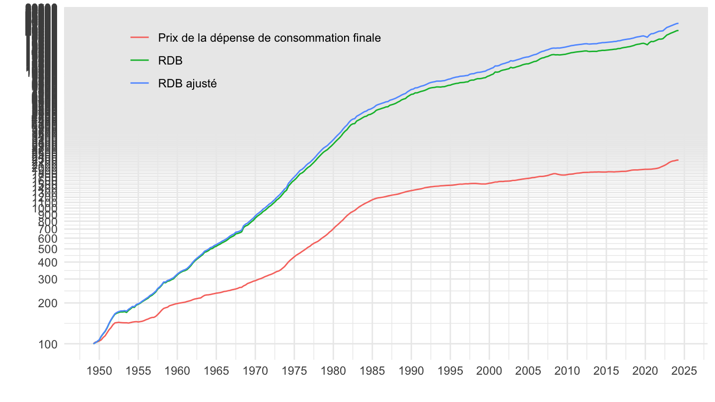
1999-
Code
t_pouvachat_val %>%
  filter(variable %in% c("P3prix", "B6", "B7")) %>%
  left_join(variable, by = "variable") %>%
  group_by(variable, Variable) %>%
  arrange(date) %>%
  filter(date >= as.Date("1999-01-01")) %>%
  mutate(index = c(100, 100*cumprod(1 + value[-1]/100))) %>%
  ggplot() + geom_line(aes(x = date, y = index, color = Variable)) +
  xlab("") + ylab("") + theme_minimal() +
  scale_x_date(breaks = as.Date(paste0(seq(1999, 2100, 5), "-01-01")),
               labels = date_format("%Y")) +
  theme(legend.position = c(0.3, 0.85),
        legend.title = element_blank()) +
  scale_y_log10(breaks = seq(100, 100000, 10)) +
  geom_label_repel(data = . %>% filter(date == max(date)),
             aes(x = date, y = index, color = Variable, label = round(index, 1)))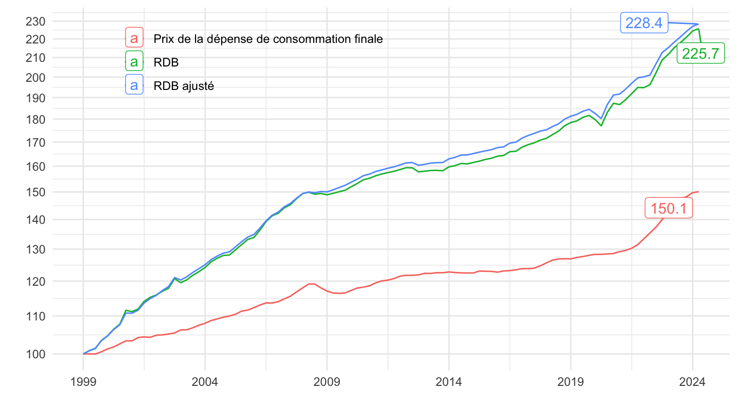
2017-
Code
t_pouvachat_val %>%
  filter(variable %in% c("P3prix", "B6", "B7")) %>%
  left_join(variable, by = "variable") %>%
  group_by(variable, Variable) %>%
  arrange(date) %>%
  filter(date >= as.Date("2017-01-01")) %>%
  mutate(index = c(100, 100*cumprod(1 + value[-1]/100))) %>%
  ggplot() + geom_line(aes(x = date, y = index, color = Variable)) +
  xlab("") + ylab("") + theme_minimal() +
  scale_x_date(breaks = as.Date(paste0(seq(1999, 2100, 1), "-01-01")),
               labels = date_format("%Y")) +
  theme(legend.position = c(0.3, 0.85),
        legend.title = element_blank()) +
  scale_y_log10(breaks = seq(100, 100000, 5)) +
  geom_label_repel(data = . %>% filter(date == max(date)),
             aes(x = date, y = index, color = Variable, label = round(index, 1)))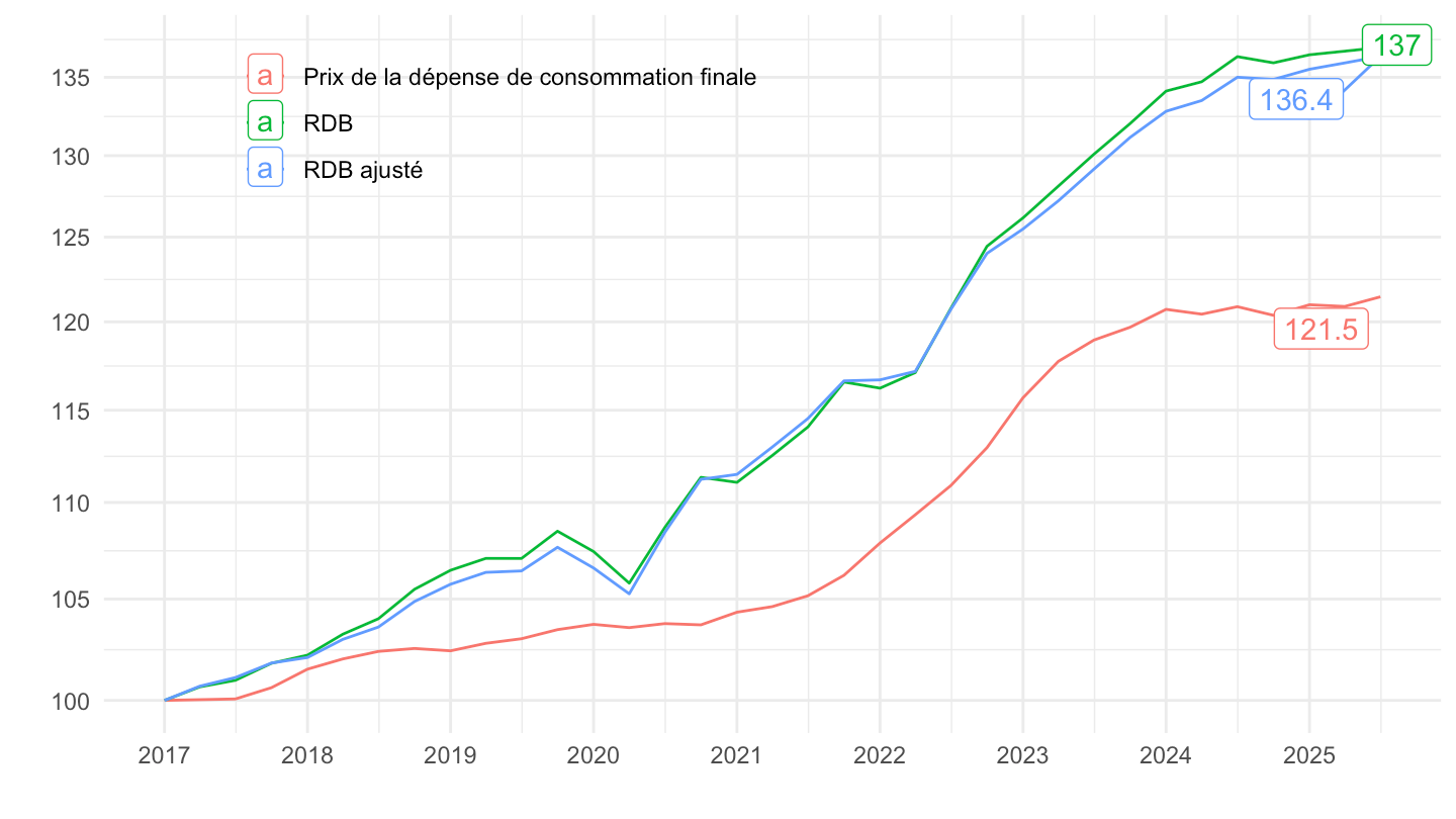
Evolution Prix de la dépense de consommation finale - P3prix
Tous
Code
t_pouvachat_val %>%
  filter(variable %in% c("P3prix", "B6", "B7")) %>%
  left_join(variable, by = "variable") %>%
  na.omit %>%
  ggplot + geom_line(aes(x = date, y = value/100, color = Variable)) +
  xlab("") + ylab("") + theme_minimal() +
  scale_x_date(breaks = seq.Date(from = as.Date("1900-01-01"), to = as.Date("2100-10-01"), by = "5 years"),
               labels = date_format("%Y")) +
  scale_y_continuous(breaks = 0.01*seq(-10, 100, 2),
                labels = percent_format(accuracy = 1)) +
  theme(legend.position = c(0.4, 0.9),
        legend.title = element_blank(),
        legend.direction = "vertical")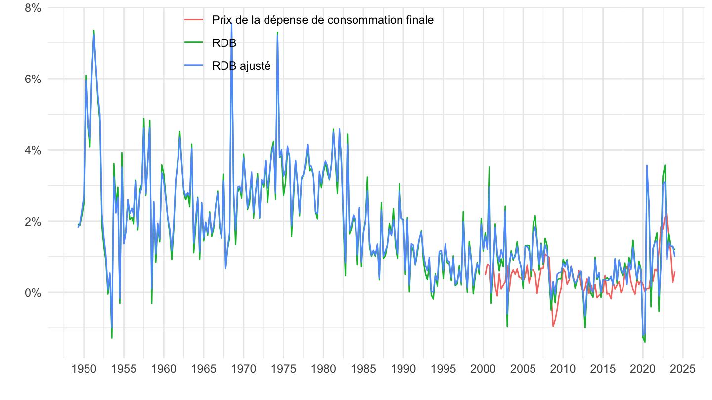
Glissement sur 1 an
Tous
Code
t_pouvachat_val %>%
  filter(variable %in% c("P3prix", "B6", "B7")) %>%
  left_join(variable, by = "variable") %>%
  na.omit %>%
  group_by(variable) %>%
  arrange(date) %>%
  mutate(value = value/100,
         ga = (1+value)*(1+lag(value,1))*(1+lag(value,2))*(1+lag(value,3))-1) %>%
  ggplot + geom_line(aes(x = date, y = ga, color = Variable)) +
  xlab("") + ylab("") + theme_minimal() +
  scale_x_date(breaks = seq.Date(from = as.Date("1900-01-01"), to = as.Date("2100-10-01"), by = "5 years"),
               labels = date_format("%Y")) +
  scale_y_continuous(breaks = 0.01*seq(-10, 100, 2),
                labels = percent_format(accuracy = 1)) +
  theme(legend.position = c(0.4, 0.9),
        legend.title = element_blank(),
        legend.direction = "vertical")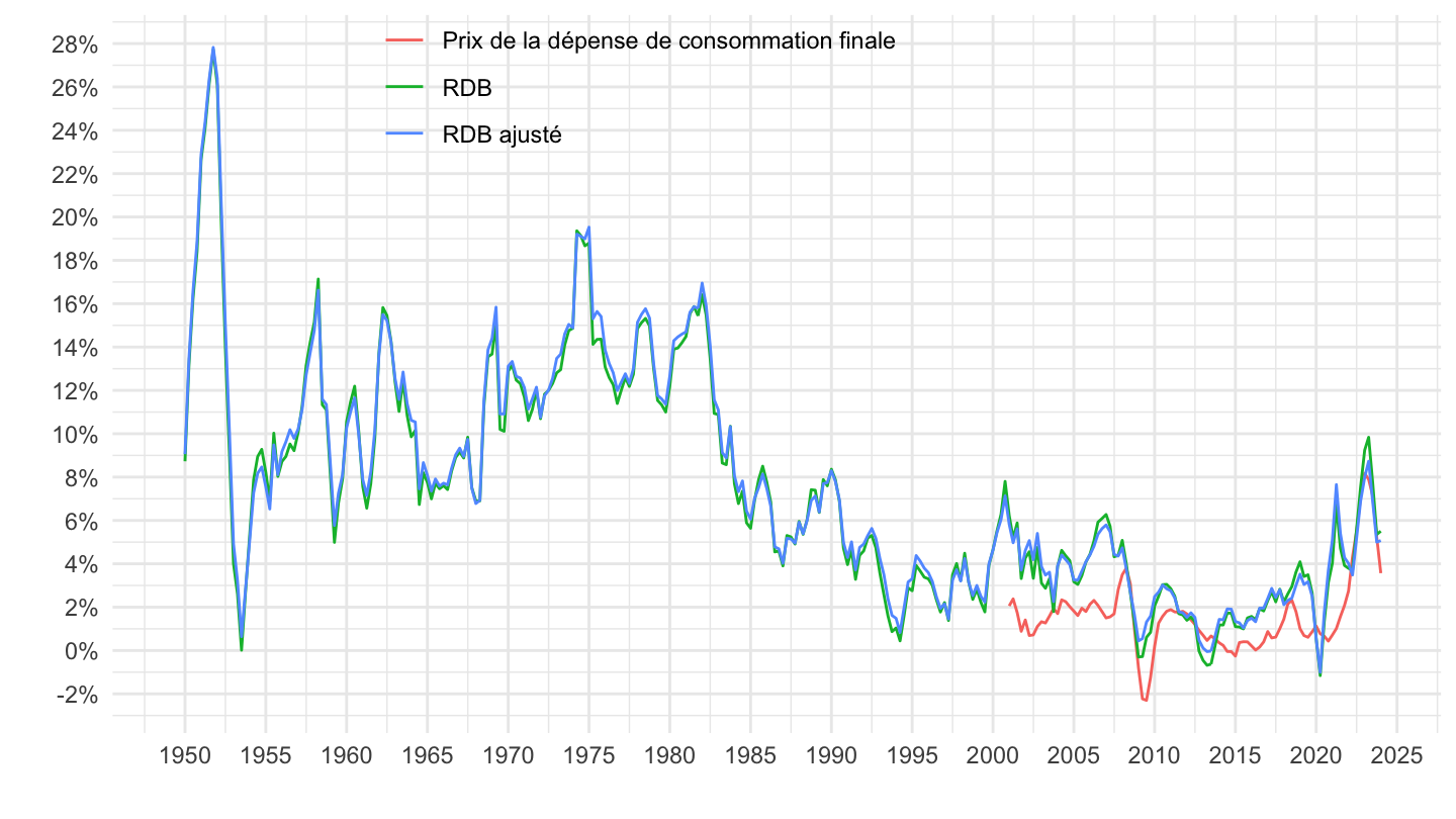
1990-
Code
t_pouvachat_val %>%
  filter(variable %in% c("P3prix", "B6", "B7")) %>%
  left_join(variable, by = "variable") %>%
  na.omit %>%
  group_by(variable) %>%
  arrange(date) %>%
  mutate(value = value/100,
         ga = (1+value)*(1+lag(value,1))*(1+lag(value,2))*(1+lag(value,3))-1) %>%
  filter(date >= as.Date("1990-01-01")) %>%
  ggplot + geom_line(aes(x = date, y = ga, color = Variable)) +
  xlab("") + ylab("") + theme_minimal() +
  scale_x_date(breaks = seq.Date(from = as.Date("1900-01-01"), to = as.Date("2100-10-01"), by = "5 years"),
               labels = date_format("%Y")) +
  scale_y_continuous(breaks = 0.01*seq(-10, 100, 1),
                labels = percent_format(accuracy = 1)) +
  theme(legend.position = c(0.4, 0.9),
        legend.title = element_blank(),
        legend.direction = "vertical")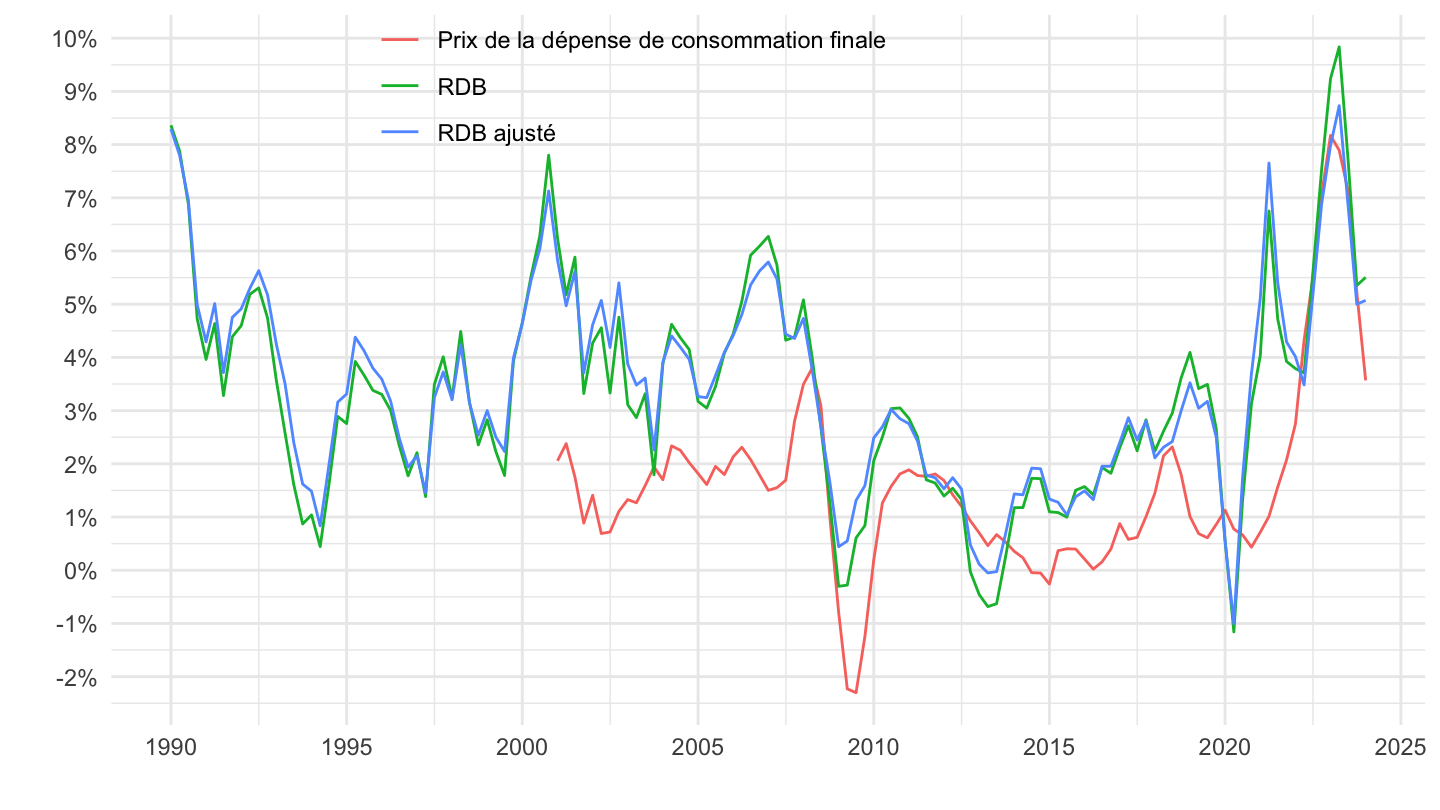
1999-
Code
t_pouvachat_val %>%
  filter(variable %in% c("P3prix", "B6", "B7")) %>%
  left_join(variable, by = "variable") %>%
  na.omit %>%
  group_by(variable) %>%
  arrange(date) %>%
  mutate(value = value/100,
         ga = (1+value)*(1+lag(value,1))*(1+lag(value,2))*(1+lag(value,3))-1) %>%
  filter(date >= as.Date("1999-01-01")) %>%
  ggplot + geom_line(aes(x = date, y = ga, color = Variable)) +
  xlab("") + ylab("") + theme_minimal() +
  scale_x_date(breaks = seq.Date(from = as.Date("1900-01-01"), to = as.Date("2100-10-01"), by = "2 years"),
               labels = date_format("%Y")) +
  scale_y_continuous(breaks = 0.01*seq(-10, 100, 1),
                labels = percent_format(accuracy = 1)) +
  theme(legend.position = c(0.4, 0.9),
        legend.title = element_blank(),
        legend.direction = "vertical")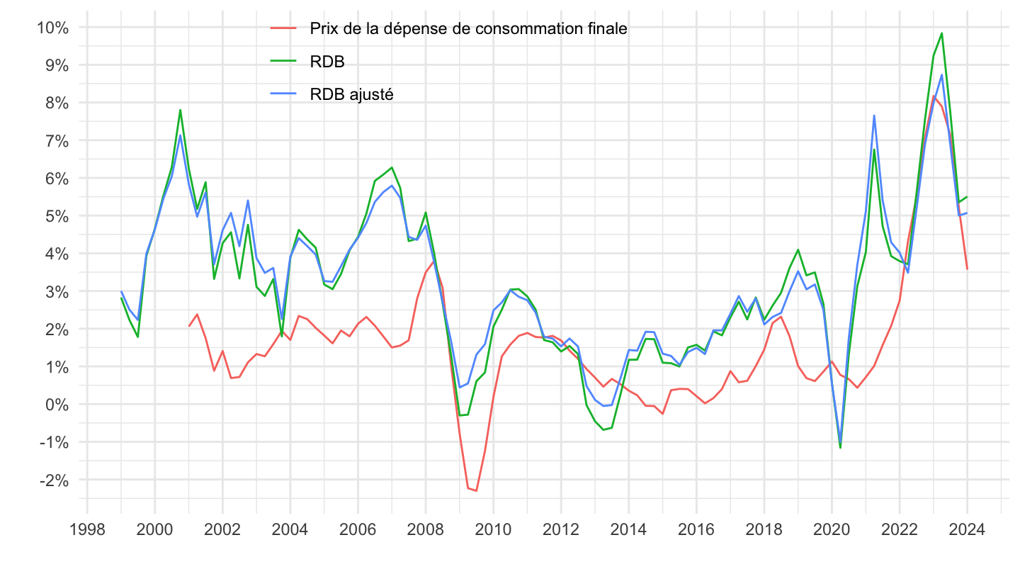
2010-
Code
t_pouvachat_val %>%
  filter(variable %in% c("P3prix", "B6", "B7")) %>%
  left_join(variable, by = "variable") %>%
  na.omit %>%
  group_by(variable) %>%
  arrange(date) %>%
  mutate(value = value/100,
         ga = (1+value)*(1+lag(value,1))*(1+lag(value,2))*(1+lag(value,3))-1) %>%
  filter(date >= as.Date("2010-01-01")) %>%
  ggplot + geom_line(aes(x = date, y = ga, color = Variable)) +
  xlab("") + ylab("") + theme_minimal() +
  scale_x_date(breaks = seq.Date(from = as.Date("1900-01-01"), to = as.Date("2100-10-01"), by = "2 years"),
               labels = date_format("%Y")) +
  scale_y_continuous(breaks = 0.01*seq(-10, 100, 1),
                labels = percent_format(accuracy = 1)) +
  theme(legend.position = c(0.4, 0.9),
        legend.title = element_blank(),
        legend.direction = "vertical")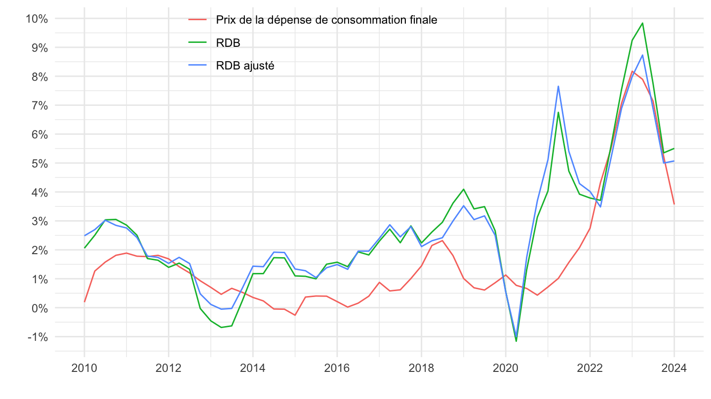
2015-
Code
t_pouvachat_val %>%
  filter(variable %in% c("P3prix", "B6", "B7")) %>%
  left_join(variable, by = "variable") %>%
  na.omit %>%
  group_by(variable) %>%
  arrange(date) %>%
  mutate(value = value/100,
         ga = (1+value)*(1+lag(value,1))*(1+lag(value,2))*(1+lag(value,3))-1) %>%
  filter(date >= as.Date("2015-01-01")) %>%
  ggplot + geom_line(aes(x = date, y = ga, color = Variable)) +
  xlab("") + ylab("") + theme_minimal() +
  scale_x_date(breaks = seq.Date(from = as.Date("1900-01-01"), to = as.Date("2100-10-01"), by = "1 year"),
               labels = date_format("%Y")) +
  scale_y_continuous(breaks = 0.01*seq(-10, 100, 1),
                labels = percent_format(accuracy = 1)) +
  theme(legend.position = c(0.4, 0.9),
        legend.title = element_blank(),
        legend.direction = "vertical")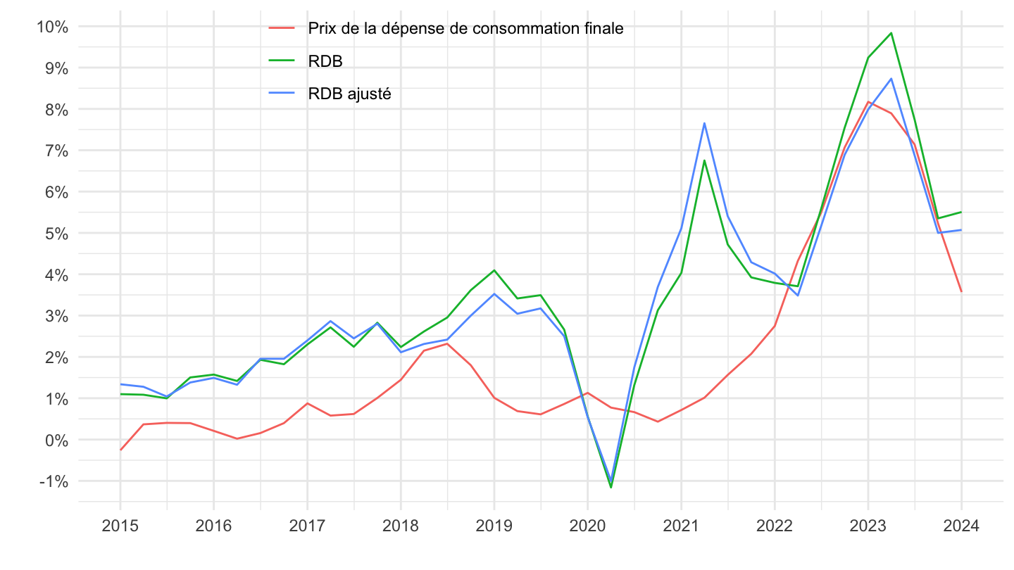
Glissement sur 2 ans
B6, B7
Code
t_pouvachat_val %>%
  filter(variable %in% c("P3prix", "B6", "B7")) %>%
  left_join(variable, by = "variable") %>%
  na.omit %>%
  group_by(variable) %>%
  arrange(date) %>%
  mutate(value = value/100,
         ga = ((1+value)*(1+lag(value,1))*(1+lag(value,2))*(1+lag(value,3))*(1+lag(value,4))*(1+lag(value,5))*(1+lag(value,6))*(1+lag(value,7)))^(1/2)-1) %>%
  ggplot + geom_line(aes(x = date, y = ga, color = Variable)) +
  xlab("") + ylab("") + theme_minimal() +
  scale_x_date(breaks = seq.Date(from = as.Date("1900-01-01"), to = as.Date("2100-10-01"), by = "5 years"),
               labels = date_format("%Y")) +
  scale_y_continuous(breaks = 0.01*seq(-10, 100, 2),
                labels = percent_format(accuracy = 1)) +
  theme(legend.position = c(0.4, 0.9),
        legend.title = element_blank(),
        legend.direction = "vertical")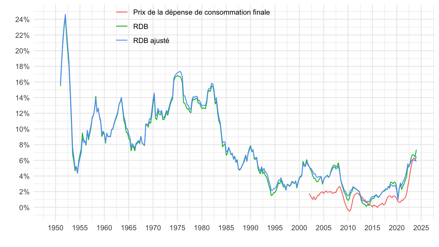
B6, B7, B6/UC
Code
t_pouvachat_val %>%
  filter(variable %in% c("P3prix", "B6", "B7", "B6/UC")) %>%
  left_join(variable, by = "variable") %>%
  na.omit %>%
  group_by(variable) %>%
  arrange(date) %>%
  mutate(value = value/100,
         ga = ((1+value)*(1+lag(value,1))*(1+lag(value,2))*(1+lag(value,3))*(1+lag(value,4))*(1+lag(value,5))*(1+lag(value,6))*(1+lag(value,7)))^(1/2)-1) %>%
  ggplot + geom_line(aes(x = date, y = ga, color = Variable)) +
  xlab("") + ylab("") + theme_minimal() +
  scale_x_date(breaks = seq.Date(from = as.Date("1900-01-01"), to = as.Date("2100-10-01"), by = "5 years"),
               labels = date_format("%Y")) +
  scale_y_continuous(breaks = 0.01*seq(-10, 100, 2),
                labels = percent_format(accuracy = 1)) +
  theme(legend.position = c(0.4, 0.9),
        legend.title = element_blank(),
        legend.direction = "vertical")
Pouvoir d’achat
Tous
Trimestriel
Code
t_pouvachat_val %>%
  filter(variable %in% c("(B6/P3prix)/UC", "(B7/P4prix)/UC")) %>%
  left_join(variable, by = "variable") %>%
  na.omit %>%
  ggplot + geom_line(aes(x = date, y = value/100, color = Variable)) +
  xlab("") + ylab("") + theme_minimal() +
  scale_x_date(breaks = seq.Date(from = as.Date("1900-01-01"), to = as.Date("2100-10-01"), by = "5 years"),
               labels = date_format("%Y")) +
  scale_y_continuous(breaks = 0.01*seq(-10, 100, 2),
                labels = percent_format(accuracy = 1)) +
  theme(legend.position = c(0.4, 0.9),
        legend.title = element_blank(),
        legend.direction = "vertical")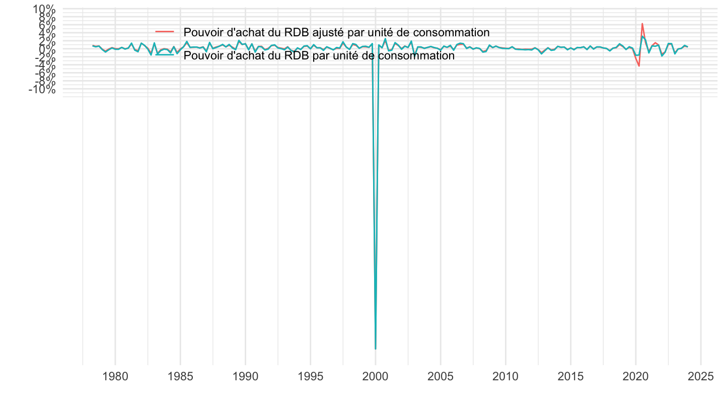
Glissement sur 1 an
Code
t_pouvachat_val %>%
  filter(variable %in% c("(B6/P3prix)/UC", "(B7/P4prix)/UC")) %>%
  left_join(variable, by = "variable") %>%
  na.omit %>%
  group_by(variable) %>%
  arrange(date) %>%
  mutate(value = value/100,
         ga = (1+value)*(1+lag(value,1))*(1+lag(value,2))*(1+lag(value,3))-1) %>%
  ggplot + geom_line(aes(x = date, y = ga, color = Variable)) +
  xlab("") + ylab("") + theme_minimal() +
  scale_x_date(breaks = seq.Date(from = as.Date("1900-01-01"), to = as.Date("2100-10-01"), by = "5 years"),
               labels = date_format("%Y")) +
  scale_y_continuous(breaks = 0.01*seq(-10, 100, 2),
                labels = percent_format(accuracy = 1)) +
  theme(legend.position = c(0.4, 0.9),
        legend.title = element_blank(),
        legend.direction = "vertical")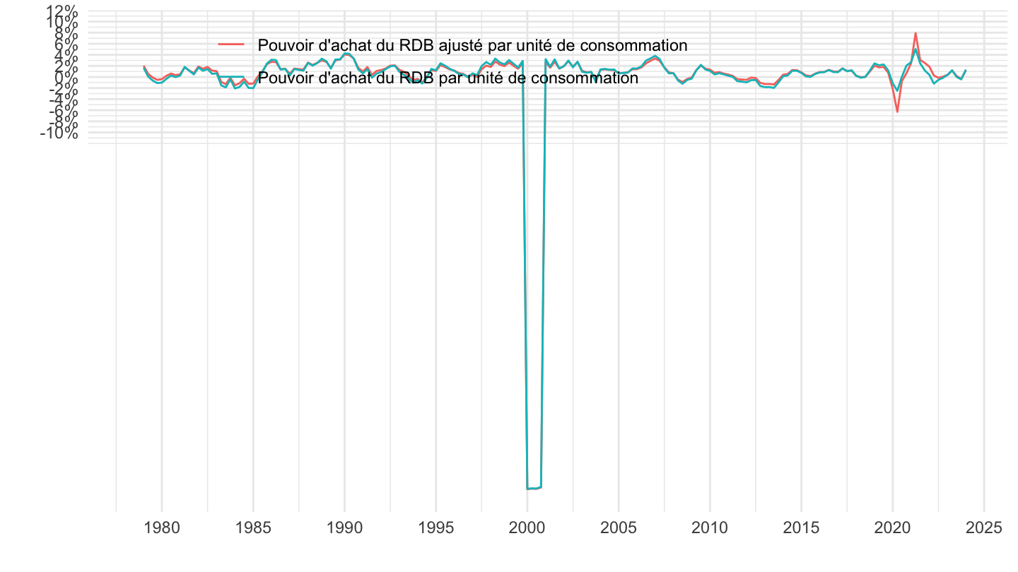
Glissement sur 2 ans
Code
t_pouvachat_val %>%
  filter(variable %in% c("(B6/P3prix)/UC", "(B7/P4prix)/UC")) %>%
  left_join(variable, by = "variable") %>%
  na.omit %>%
  group_by(variable) %>%
  arrange(date) %>%
  mutate(value = value/100,
         ga = ((1+value)*(1+lag(value,1))*(1+lag(value,2))*(1+lag(value,3))*(1+lag(value,4))*(1+lag(value,5))*(1+lag(value,6))*(1+lag(value,7)))^(1/2)-1) %>%
  ggplot + geom_line(aes(x = date, y = ga, color = Variable)) +
  xlab("") + ylab("") + theme_minimal() +
  scale_x_date(breaks = seq.Date(from = as.Date("1900-01-01"), to = as.Date("2100-10-01"), by = "5 years"),
               labels = date_format("%Y")) +
  scale_y_continuous(breaks = 0.01*seq(-10, 100, 1),
                labels = percent_format(accuracy = 1)) +
  theme(legend.position = c(0.4, 0.9),
        legend.title = element_blank(),
        legend.direction = "vertical")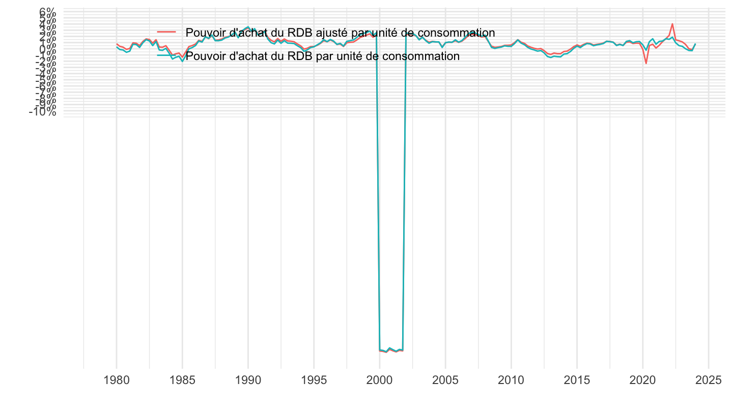
Glissement sur 3 ans
Code
t_pouvachat_val %>%
  filter(variable %in% c("(B6/P3prix)/UC", "(B7/P4prix)/UC")) %>%
  left_join(variable, by = "variable") %>%
  na.omit %>%
  group_by(variable) %>%
  arrange(date) %>%
  mutate(value = value/100,
         ga = ((1+value)*(1+lag(value,1))*(1+lag(value,2))*(1+lag(value,3))*(1+lag(value,4))*(1+lag(value,5))*(1+lag(value,6))*(1+lag(value,7))*(1+lag(value,8))*(1+lag(value,9))*(1+lag(value,10))*(1+lag(value,11)))^(1/3)-1) %>%
  ggplot + geom_line(aes(x = date, y = ga, color = Variable)) +
  xlab("") + ylab("") + theme_minimal() +
  scale_x_date(breaks = seq.Date(from = as.Date("1900-01-01"), to = as.Date("2100-10-01"), by = "5 years"),
               labels = date_format("%Y")) +
  scale_y_continuous(breaks = 0.01*seq(-10, 100, 1),
                labels = percent_format(accuracy = 1)) +
  theme(legend.position = c(0.4, 0.9),
        legend.title = element_blank(),
        legend.direction = "vertical")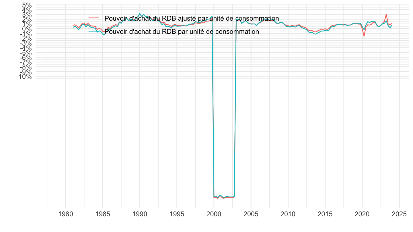
Glissement sur 4 ans
Code
t_pouvachat_val %>%
  filter(variable %in% c("(B6/P3prix)/UC", "(B7/P4prix)/UC")) %>%
  left_join(variable, by = "variable") %>%
  na.omit %>%
  group_by(variable) %>%
  arrange(date) %>%
  mutate(value = value/100,
         ga = ((1+value)*(1+lag(value,1))*(1+lag(value,2))*(1+lag(value,3))*(1+lag(value,4))*(1+lag(value,5))*(1+lag(value,6))*(1+lag(value,7))*(1+lag(value,8))*(1+lag(value,9))*(1+lag(value,10))*(1+lag(value,11))*(1+lag(value,12))*(1+lag(value,13))*(1+lag(value,14))*(1+lag(value,15)))^(1/4)-1) %>%
  ggplot + geom_line(aes(x = date, y = ga, color = Variable)) +
  xlab("") + ylab("") + theme_minimal() +
  scale_x_date(breaks = seq.Date(from = as.Date("1900-01-01"), to = as.Date("2100-10-01"), by = "5 years"),
               labels = date_format("%Y")) +
  scale_y_continuous(breaks = 0.01*seq(-10, 100, 1),
                labels = percent_format(accuracy = 1)) +
  theme(legend.position = c(0.4, 0.9),
        legend.title = element_blank(),
        legend.direction = "vertical")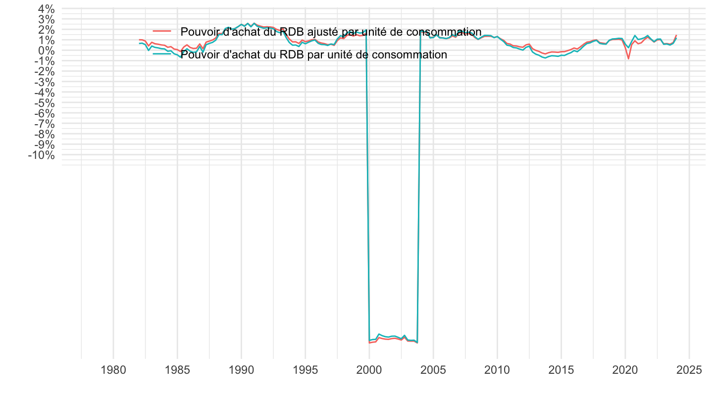
Glissement sur 5 ans
Code
t_pouvachat_val %>%
  filter(variable %in% c("(B6/P3prix)/UC", "(B7/P4prix)/UC")) %>%
  left_join(variable, by = "variable") %>%
  na.omit %>%
  group_by(variable) %>%
  arrange(date) %>%
  mutate(value = value/100,
         ga = ((1+value)*(1+lag(value,1))*(1+lag(value,2))*(1+lag(value,3))*(1+lag(value,4))*(1+lag(value,5))*(1+lag(value,6))*(1+lag(value,7))*(1+lag(value,8))*(1+lag(value,9))*(1+lag(value,10))*(1+lag(value,11))*(1+lag(value,12))*(1+lag(value,13))*(1+lag(value,14))*(1+lag(value,15))*(1+lag(value,16))*(1+lag(value,17))*(1+lag(value,18))*(1+lag(value,19)))^(1/5)-1) %>%
  ggplot + geom_line(aes(x = date, y = ga, color = Variable)) +
  xlab("") + ylab("") + theme_minimal() +
  scale_x_date(breaks = seq.Date(from = as.Date("1900-01-01"), to = as.Date("2100-10-01"), by = "5 years"),
               labels = date_format("%Y")) +
  scale_y_continuous(breaks = 0.01*seq(-10, 100, 1),
                labels = percent_format(accuracy = 1)) +
  theme(legend.position = c(0.4, 0.9),
        legend.title = element_blank(),
        legend.direction = "vertical")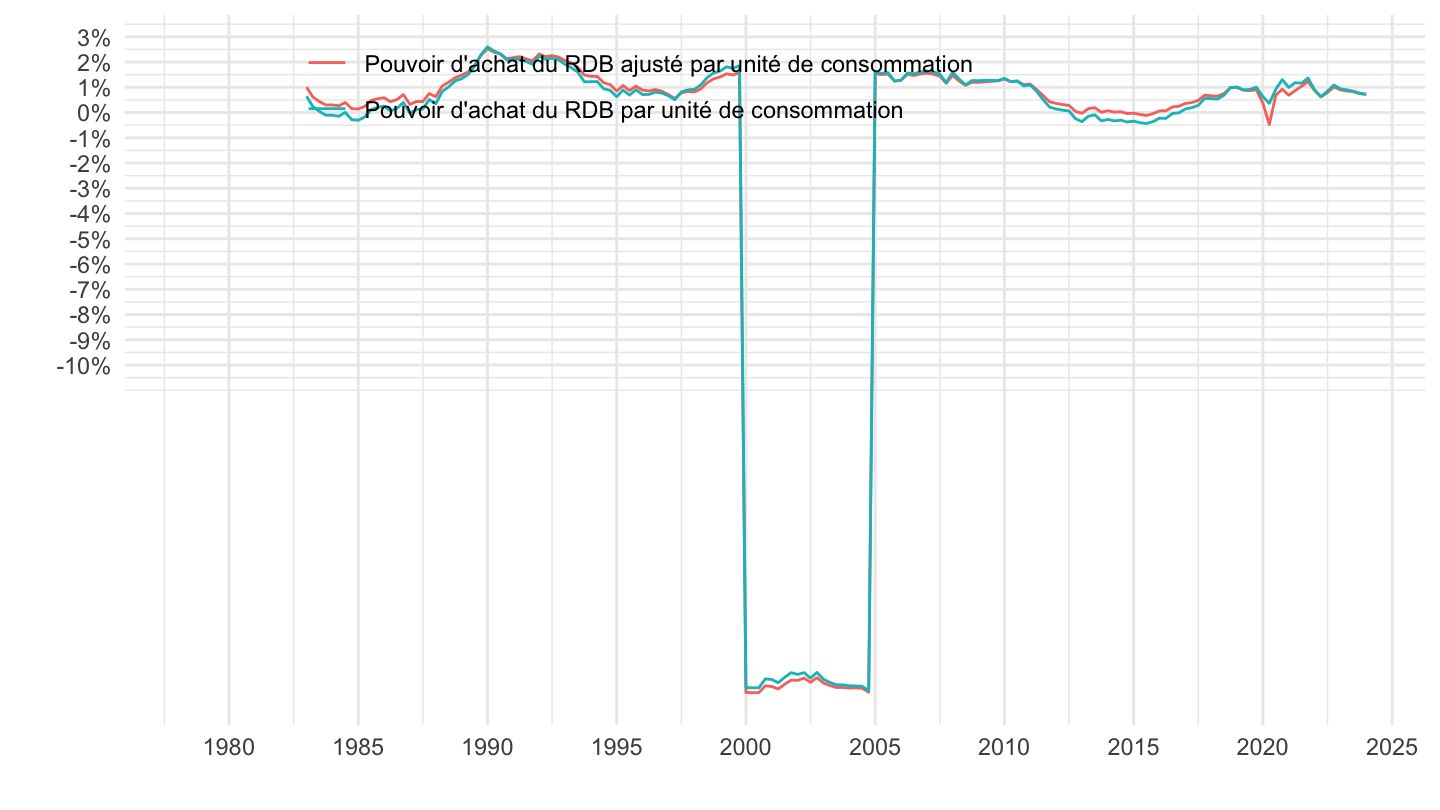
2017T2-
Code
t_pouvachat_val %>%
  filter(variable %in% c("(B6/P3prix)/UC", "(B7/P4prix)/UC", "B6 / P3prix", "B7/P4prix"),
         date >= as.Date("2017-04-01")) %>%
  mutate(date = zoo::as.yearqtr(date)) %>%
  left_join(variable, by = "variable") %>%
  na.omit %>%
  ggplot + geom_line(aes(x = date, y = value/100, color = Variable)) +
  xlab("") + ylab("") + theme_minimal() +
  zoo::scale_x_yearqtr(labels = date_format("%YT%q"),
                       breaks = expand.grid(2017:2100, c(2, 4)) %>%
                         mutate(breaks = zoo::as.yearqtr(paste0(Var1, "Q", Var2))) %>%
                         pull(breaks)) +
  scale_y_continuous(breaks = 0.01*seq(-10, 100, 1),
                labels = percent_format(accuracy = 1)) +
  theme(legend.position = c(0.4, 0.8),
        legend.title = element_blank(),
        axis.text.x = element_text(angle = 45, vjust = 1, hjust = 1))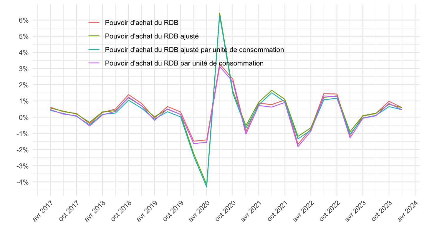
3 years
Code
t_pouvachat_val %>%
  filter(variable %in% c("(B6/P3prix)/UC", "(B7/P4prix)/UC", "B6 / P3prix", "B7/P4prix"),
         date >= max(date) - years(3)) %>%
  mutate(date = zoo::as.yearqtr(date)) %>%
  left_join(variable, by = "variable") %>%
  na.omit %>%
  ggplot + geom_line(aes(x = date, y = value/100, color = Variable)) +
  xlab("") + ylab("") + theme_minimal() +
  zoo::scale_x_yearqtr(labels = date_format("%YT%q"),
                       breaks = expand.grid(2017:2100, 1:4) %>%
                         mutate(breaks = zoo::as.yearqtr(paste0(Var1, "Q", Var2))) %>%
                         pull(breaks)) +
  scale_y_continuous(breaks = 0.01*seq(-10, 100, 1),
                labels = percent_format(accuracy = 1)) +
  theme(legend.position = c(0.4, 0.8),
        legend.title = element_blank(),
        axis.text.x = element_text(angle = 45, vjust = 1, hjust = 1))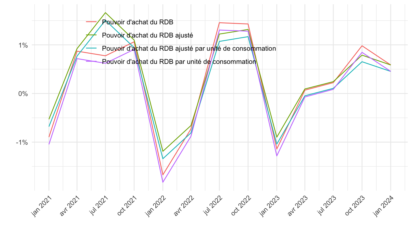
2 years
Trimestriel
Code
t_pouvachat_val %>%
  filter(variable %in% c("(B6/P3prix)/UC", "(B7/P4prix)/UC", "B6 / P3prix", "B7/P4prix"),
         date >= max(date) - years(2)) %>%
  mutate(date = zoo::as.yearqtr(date)) %>%
  left_join(variable, by = "variable") %>%
  na.omit %>%
  ggplot + geom_line(aes(x = date, y = value/100, color = Variable)) +
  xlab("") + ylab("") + theme_minimal() +
  zoo::scale_x_yearqtr(labels = date_format("%YT%q"),
                       breaks = expand.grid(2017:2100, 1:4) %>%
                         mutate(breaks = zoo::as.yearqtr(paste0(Var1, "Q", Var2))) %>%
                         pull(breaks)) +
  scale_y_continuous(breaks = 0.01*seq(-10, 100, 1),
                labels = percent_format(accuracy = 1)) +
  theme(legend.position = c(0.4, 0.8),
        legend.title = element_blank(),
        axis.text.x = element_text(angle = 45, vjust = 1, hjust = 1))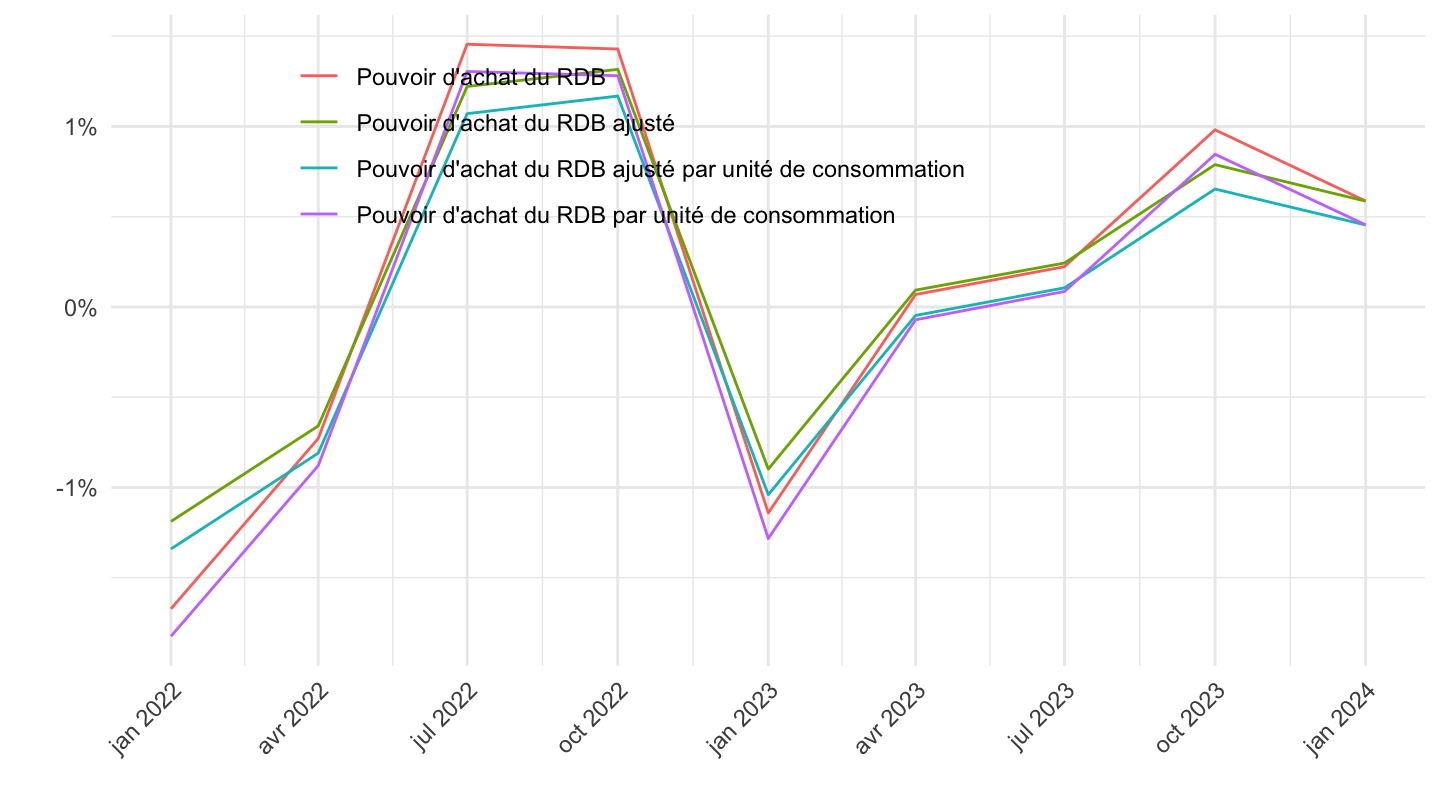
Glissement sur 1 an
Code
t_pouvachat_val %>%
  filter(variable %in% c("(B6/P3prix)/UC", "(B7/P4prix)/UC", "B6 / P3prix", "B7/P4prix")) %>%
  left_join(variable, by = "variable") %>%
  na.omit %>%
  group_by(variable) %>%
  arrange(date) %>%
  mutate(value = value/100,
         ga = (1+value)*(1+lag(value,1))*(1+lag(value,2))*(1+lag(value,3))-1) %>%
  filter(date >= max(date) - years(2)) %>%
  ggplot + geom_line(aes(x = date, y = ga, color = Variable)) +
  xlab("") + ylab("") + theme_minimal() +
  scale_x_date(breaks = seq.Date(from = as.Date("1990-01-01"), to = as.Date("2100-10-01"), by = "3 months"),
               labels = date_format("%b %Y")) +
  scale_y_continuous(breaks = 0.01*seq(-10, 100, 1),
                labels = percent_format(accuracy = 1)) +
  theme(legend.position = c(0.7, 0.85),
        legend.title = element_blank(),
        axis.text.x = element_text(angle = 45, vjust = 1, hjust = 1))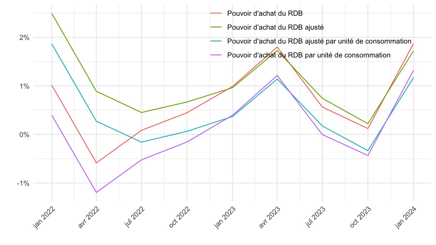
Taux d’épargne vs. d’épargne financière
Tous
Code
t_pouvachat_val %>%
  filter(variable %in% c("B9NF/(B6+D8)", "B8/(B6+D8)")) %>%
  left_join(variable, by = "variable") %>%
  na.omit %>%
  ggplot + geom_line(aes(x = date, y = value/100, color = Variable)) +
  xlab("") + ylab("") + theme_minimal() +
  scale_x_date(breaks = seq.Date(from = as.Date("1900-01-01"), to = as.Date("2100-10-01"), by = "5 years"),
               labels = date_format("%Y")) +
  scale_y_continuous(breaks = 0.01*seq(-10, 100, 2),
                labels = percent_format(accuracy = 1)) +
  theme(legend.position = c(0.2, 0.9),
        legend.title = element_blank(),
        legend.direction = "vertical")
1995-
Code
t_pouvachat_val %>%
  filter(variable %in% c("B9NF/(B6+D8)", "B8/(B6+D8)"),
         date >= as.Date("1995-01-01")) %>%
  left_join(variable, by = "variable") %>%
  na.omit %>%
  mutate(date = zoo::as.yearqtr(date, format = "%YT%q")) %>%
  ggplot + geom_line(aes(x = date, y = value/100, color = Variable)) +
  xlab("") + ylab("") + theme_minimal() +
  scale_x_yearqtr() +
  scale_y_continuous(breaks = 0.01*seq(-10, 100, 2),
                labels = percent_format(accuracy = 1)) +
  theme(legend.position = c(0.2, 0.9),
        legend.title = element_blank(),
        legend.direction = "vertical")
2005-
Code
t_pouvachat_val %>%
  filter(variable %in% c("B9NF/(B6+D8)", "B8/(B6+D8)"),
         date >= as.Date("2005-01-01")) %>%
  left_join(variable, by = "variable") %>%
  na.omit %>%
  mutate(date = zoo::as.yearqtr(date, format = "%YT%q")) %>%
  ggplot + geom_line(aes(x = date, y = value/100, color = Variable)) +
  xlab("") + ylab("") + theme_minimal() +
  scale_x_yearqtr() +
  scale_y_continuous(breaks = 0.01*seq(-10, 100, 2),
                labels = percent_format(accuracy = 1)) +
  theme(legend.position = c(0.2, 0.9),
        legend.title = element_blank(),
        legend.direction = "vertical")
2012-
Code
t_pouvachat_val %>%
  filter(variable %in% c("B9NF/(B6+D8)", "B8/(B6+D8)"),
         date >= as.Date("2012-01-01")) %>%
  left_join(variable, by = "variable") %>%
  na.omit %>%
  mutate(date = zoo::as.yearqtr(date, format = "%YT%q")) %>%
  ggplot + geom_line(aes(x = date, y = value/100, color = Variable)) +
  xlab("") + ylab("") + theme_minimal() +
  scale_x_yearqtr() +
  scale_y_continuous(breaks = 0.01*seq(-10, 100, 2),
                labels = percent_format(accuracy = 1)) +
  theme(legend.position = c(0.2, 0.9),
        legend.title = element_blank(),
        legend.direction = "vertical")
2017T2-
Code
t_pouvachat_val %>%
  filter(variable %in% c("B9NF/(B6+D8)", "B8/(B6+D8)"),
         date >= as.Date("2017-04-01")) %>%
  left_join(variable, by = "variable") %>%
  na.omit %>%
  mutate(date = zoo::as.yearqtr(date, format = "%YT%q")) %>%
  ggplot + geom_line(aes(x = date, y = value/100, color = Variable)) +
  xlab("") + ylab("") + theme_minimal() +
  scale_x_yearqtr(labels = date_format("%Y-T%q"),
                       breaks = expand.grid(2017:2100, c(2, 4)) %>%
                         mutate(breaks = zoo::as.yearqtr(paste0(Var1, "Q", Var2))) %>%
                         pull(breaks)) +
  scale_y_continuous(breaks = 0.01*seq(-10, 100, 2),
                labels = percent_format(accuracy = 1)) +
  theme(legend.position = c(0.2, 0.9),
        legend.title = element_blank(),
        legend.direction = "vertical",
        axis.text.x = element_text(angle = 45, vjust = 1, hjust = 1))
Taux d’épargne
2012-
Code
t_pouvachat_val %>%
  filter(variable %in% c("B8/(B6+D8)"),
         date >= as.Date("2014-01-01")) %>%
  left_join(variable, by = "variable") %>%
  na.omit %>%
  ggplot + geom_line(aes(x = date, y = value/100, color = Variable)) +
  xlab("") + ylab("Taux d'épargne (%)") + theme_minimal() +
  scale_x_date(breaks = seq.Date(from = as.Date("1995-01-01"), to = as.Date("2100-10-01"), by = "1 year"),
               labels = date_format("%Y")) +
  scale_y_continuous(breaks = 0.01*seq(-10, 100, 1),
                labels = percent_format(accuracy = 1)) +
  theme(legend.position = c(0.2, 0.9),
        legend.title = element_blank(),
        legend.direction = "vertical")