Target Balances
Data - ECB
Info
Data on monetary policy
| source | dataset | Title | .html | .rData |
|---|---|---|---|---|
| ecb | ILM_PUB | Internal Liquidity Management - Published series | 2026-07-23 | 2026-07-22 |
| bdf | FM | Marché financier, taux | 2026-07-22 | 2026-07-22 |
| bdf | MIR | Taux d'intérêt - Zone euro | 2026-07-22 | 2026-07-22 |
| bdf | MIR1 | Taux d'intérêt - France | 2026-07-23 | 2026-07-23 |
| bis | CBPOL | Policy Rates, Daily | 2026-07-18 | 2026-07-22 |
| ecb | BSI | Balance Sheet Items | 2026-07-23 | 2026-07-22 |
| ecb | BSI_PUB | Balance Sheet Items - Published series | 2026-07-23 | 2026-07-22 |
| ecb | FM | Financial market data | 2026-07-23 | 2026-07-22 |
| ecb | ILM | Internal Liquidity Management | 2026-07-23 | 2026-07-22 |
| ecb | MIR | MFI Interest Rate Statistics | 2026-07-23 | 2026-07-22 |
| ecb | RAI | Risk Assessment Indicators | 2026-07-23 | 2026-07-23 |
| ecb | SUP | Supervisory Banking Statistics | 2026-07-23 | 2026-07-23 |
| ecb | YC | Financial market data - yield curve | 2026-07-23 | 2026-07-23 |
| ecb | YC_PUB | Financial market data - yield curve - Published series | 2026-07-23 | 2026-07-23 |
| ecb | liq_daily | Daily Liquidity | 2026-07-23 | 2026-07-23 |
| eurostat | ei_mfir_m | Interest rates - monthly data | 2026-07-23 | 2026-07-23 |
| eurostat | irt_st_m | Money market interest rates - monthly data | 2026-07-23 | 2026-07-23 |
| fred | r | Interest Rates | 2026-07-22 | 2026-07-22 |
| oecd | MEI | Main Economic Indicators | 2024-04-16 | 2025-07-24 |
| oecd | MEI_FIN | Monthly Monetary and Financial Statistics (MEI) | 2024-09-15 | 2025-07-24 |
LAST_COMPILE
| LAST_COMPILE |
|---|
| 2026-07-24 |
Last
| TIME_PERIOD | FREQ | Nobs |
|---|---|---|
| 2026-05 | M | 46 |
FREQ
Code
TGB %>%
  group_by(FREQ) %>%
  summarise(Nobs = n()) %>%
  arrange(-Nobs) %>%
{if (is_html_output()) print_table(.) else .}| FREQ | Nobs |
|---|---|
| M | 11494 |
REF_AREA
Code
TGB %>%
  left_join(REF_AREA, by = "REF_AREA") %>%
  group_by(REF_AREA, Ref_area) %>%
  summarise(Nobs = n()) %>%
  arrange(-Nobs) %>%
  mutate(Loc = gsub(" ", "-", str_to_lower(Ref_area)),
         Loc = paste0('<img src="../../icon/flag/vsmall/', Loc, '.png" alt="Flag">')) %>%
  select(Loc, everything()) %>%
  {if (is_html_output()) datatable(., filter = 'top', rownames = F, escape = F) else .}
TIME_PER_COLLECT
Code
TGB %>%
  group_by(TIME_PER_COLLECT) %>%
  summarise(Nobs = n()) %>%
  arrange(-Nobs) %>%
{if (is_html_output()) print_table(.) else .}| TIME_PER_COLLECT | Nobs |
|---|---|
| A | 6715 |
| E | 4779 |
TIME_PERIOD
Code
TGB %>%
  group_by(TIME_PERIOD) %>%
  summarise(Nobs = n()) %>%
  arrange(desc(TIME_PERIOD)) %>%
  print_table_conditional()
Target Balances
Table
Code
TGB %>%
  filter(TIME_PER_COLLECT == "A",
         TIME_PERIOD %in% c("2019-02", "2020-06", "2020-10", max(TIME_PERIOD))) %>%
  left_join(REF_AREA, by = "REF_AREA") %>%
  mutate(Ref_area = ifelse(REF_AREA == "4F", "Europe", Ref_area),
         OBS_VALUE = round(OBS_VALUE)) %>%
  select(REF_AREA, Ref_area, TIME_PERIOD, OBS_VALUE) %>%
  spread(TIME_PERIOD, OBS_VALUE) %>%
  mutate(Change = `2020-10`-`2019-02`) %>%
  mutate(Loc = gsub(" ", "-", str_to_lower(Ref_area)),
         Loc = paste0('<img src="../../icon/flag/vsmall/', Loc, '.png" alt="Flag">')) %>%
  select(Loc, everything()) %>%
  {if (is_html_output()) datatable(., filter = 'top', rownames = F, escape = F) else .}
France, Germany, Italy, Greece
Tous
Code
TGB %>%
  filter(REF_AREA %in% c("FR", "DE", "IT", "GR"),
         TIME_PER_COLLECT == "A") %>%
  left_join(REF_AREA, by = "REF_AREA") %>%
  month_to_date() %>%
  filter(!is.na(OBS_VALUE)) %>%
  mutate(OBS_VALUE = OBS_VALUE/1000) %>%
  left_join(colors, by = c("Ref_area" = "country")) %>%
  mutate(color = ifelse(REF_AREA == "U2", color2, color)) %>%
  ggplot() + theme_minimal() +
  geom_line(aes(x = date, y = OBS_VALUE, color = color)) +
  add_flags(4) + scale_color_identity() +
  scale_x_date(breaks = seq(1920, 2100, 2) %>% paste0("-01-01") %>% as.Date,
               labels = date_format("%Y")) +
  theme(legend.position = c(0.35, 0.85),
        legend.title = element_blank()) +
  scale_y_continuous(breaks = seq(-3000, 3000, 100),
                     labels = dollar_format(accuracy = 1, prefix = "", suffix = " Bn€")) +
  ylab("Target Balances") + xlab("")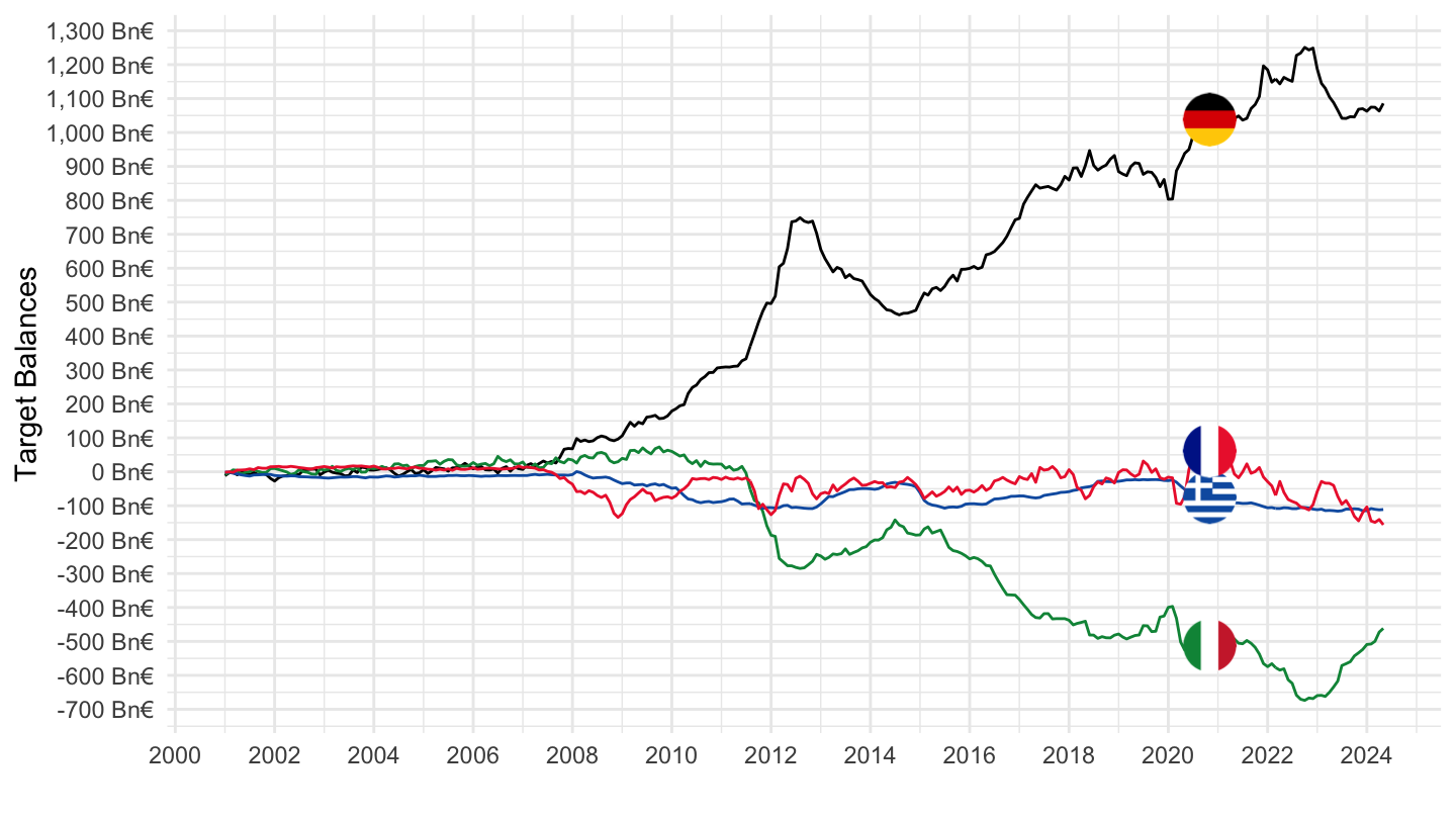
2010
Code
TGB %>%
  filter(REF_AREA %in% c("FR", "DE", "IT", "GR"),
         TIME_PER_COLLECT == "A") %>%
  left_join(REF_AREA, by = "REF_AREA") %>%
  month_to_date() %>%
  filter(date >= as.Date("2010-01-01")) %>%
  filter(!is.na(OBS_VALUE)) %>%
  mutate(OBS_VALUE = OBS_VALUE/1000) %>%
  left_join(colors, by = c("Ref_area" = "country")) %>%
  mutate(color = ifelse(REF_AREA == "U2", color2, color)) %>%
  ggplot() + theme_minimal() +
  geom_line(aes(x = date, y = OBS_VALUE, color = color)) +
  add_flags(4) + scale_color_identity() +
  scale_x_date(breaks = seq(1920, 2100, 2) %>% paste0("-01-01") %>% as.Date,
               labels = date_format("%Y")) +
  theme(legend.position = c(0.35, 0.85),
        legend.title = element_blank()) +
  scale_y_continuous(breaks = seq(-3000, 3000, 100),
                     labels = dollar_format(accuracy = 1, prefix = "", suffix = " Bn€")) +
  ylab("Target Balances") + xlab("")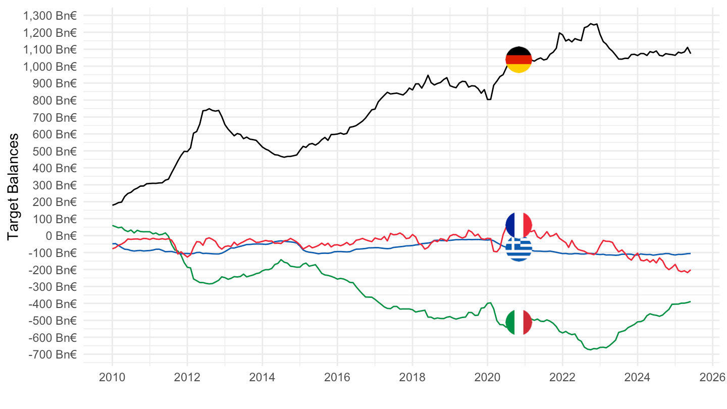
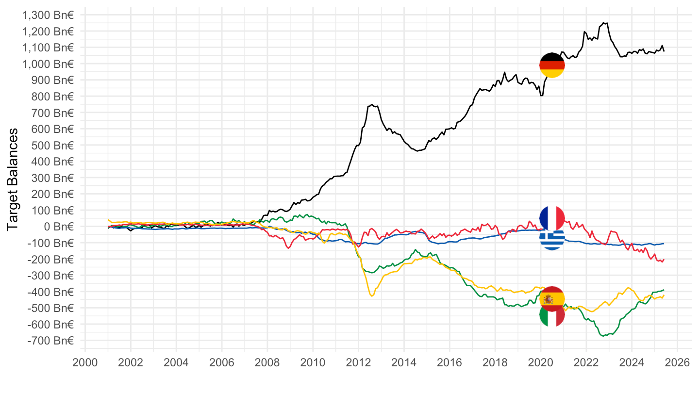
France, Germany, Italy, Greece, Spain,
Code
TGB %>%
  filter(REF_AREA %in% c("FR", "DE", "IT", "GR", "ES"),
         TIME_PER_COLLECT == "A") %>%
  left_join(REF_AREA, by = "REF_AREA") %>%
  month_to_date() %>%
  filter(!is.na(OBS_VALUE)) %>%
  mutate(OBS_VALUE = OBS_VALUE/1000) %>%
  left_join(colors, by = c("Ref_area" = "country")) %>%
  mutate(color = ifelse(REF_AREA == "U2", color2, color)) %>%
  ggplot() + theme_minimal() +
  geom_line(aes(x = date, y = OBS_VALUE, color = color)) +
  add_flags(5) + scale_color_identity() +
  scale_x_date(breaks = seq(1920, 2100, 2) %>% paste0("-01-01") %>% as.Date,
               labels = date_format("%Y")) +
  theme(legend.position = c(0.35, 0.85),
        legend.title = element_blank()) +
  scale_y_continuous(breaks = seq(-3000, 3000, 100),
                     labels = dollar_format(accuracy = 1, prefix = "", suffix = " Bn€")) +
  ylab("Target Balances") + xlab("")