Unit Labour Costs - Annual Indicators
Data - OECD
Info
Data on industry
| source | dataset | Title | .html | .rData |
|---|---|---|---|---|
| ec | INDUSTRY | Industry (sector data) | 2026-07-24 | 2026-07-24 |
| eurostat | ei_isin_m | Industry - monthly data - index (2015 = 100) (NACE Rev. 2) - ei_isin_m | 2026-07-22 | 2026-07-23 |
| eurostat | htec_trd_group4 | High-tech trade by high-tech group of products in million euro (from 2007, SITC Rev. 4) | 2026-07-22 | 2026-07-23 |
| eurostat | nama_10_a64 | National accounts aggregates by industry (up to NACE A*64) | 2026-07-17 | 2026-07-23 |
| eurostat | nama_10_a64_e | National accounts employment data by industry (up to NACE A*64) | 2026-07-24 | 2026-07-24 |
| eurostat | namq_10_a10_e | Employment A*10 industry breakdowns | 2026-07-24 | 2026-07-24 |
| eurostat | road_eqr_carmot | New registrations of passenger cars by type of motor energy and engine size - road_eqr_carmot | 2026-07-24 | 2026-07-23 |
| eurostat | sts_inpp_m | Producer prices in industry, total - monthly data | 2026-07-21 | 2026-07-24 |
| eurostat | sts_inppd_m | Producer prices in industry, domestic market - monthly data | 2026-07-21 | 2026-07-24 |
| eurostat | sts_inpr_m | Production in industry - monthly data | 2026-07-21 | 2026-07-23 |
| eurostat | sts_intvnd_m | Turnover in industry, non domestic market - monthly data - sts_intvnd_m | 2026-07-24 | 2026-07-24 |
| fred | industry | Manufacturing, Industry | 2026-07-24 | 2026-07-24 |
| oecd | ALFS_EMP | Employment by activities and status (ALFS) | 2026-07-24 | 2025-05-24 |
| oecd | BERD_MA_SOF | Business enterprise R&D expenditure by main activity (focussed) and source of funds | 2026-07-24 | 2023-09-09 |
| oecd | GBARD_NABS2007 | Government budget allocations for R and D | 2024-04-16 | 2023-11-22 |
| oecd | MEI_REAL | Production and Sales (MEI) | 2024-05-12 | 2025-05-24 |
| oecd | MSTI_PUB | Main Science and Technology Indicators | 2024-09-15 | 2025-05-24 |
| oecd | SNA_TABLE4 | PPPs and exchange rates | 2024-09-15 | 2025-05-24 |
| wdi | NV.IND.EMPL.KD | Industry, value added per worker (constant 2010 USD) | 2026-07-25 | 2026-07-24 |
| wdi | NV.IND.MANF.CD | Manufacturing, value added (current USD) | 2026-07-25 | 2026-07-24 |
| wdi | NV.IND.MANF.ZS | Manufacturing, value added (% of GDP) | 2026-07-25 | 2026-07-24 |
| wdi | NV.IND.TOTL.KD | Industry (including construction), value added (constant 2015 USD) - NV.IND.TOTL.KD | 2026-07-25 | 2026-07-24 |
| wdi | NV.IND.TOTL.ZS | Industry, value added (including construction) (% of GDP) | 2026-07-25 | 2026-07-24 |
| wdi | SL.IND.EMPL.ZS | Employment in industry (% of total employment) | 2026-07-25 | 2026-07-24 |
| wdi | TX.VAL.MRCH.CD.WT | Merchandise exports (current USD) | 2026-07-25 | 2026-07-24 |
LAST_COMPILE
| LAST_COMPILE |
|---|
| 2026-07-26 |
Last
| obsTime | Nobs |
|---|---|
| 2012 | 1177 |
Nobs
Code
ULC_ANN %>%
  left_join(ULC_ANN_var$SUBJECT, by = "SUBJECT") %>%
  left_join(ULC_ANN_var$SECTOR, by = "SECTOR") %>%
  group_by(SUBJECT, Subject, SECTOR, Sector, MEASURE) %>%
  summarise(Nobs = n()) %>%
  arrange(-Nobs) %>%
  print_table_conditional()
SUBJECT
Code
ULC_ANN %>%
  left_join(ULC_ANN_var$SUBJECT, by = "SUBJECT") %>%
  group_by(SUBJECT, Subject) %>%
  summarise(Nobs = n()) %>%
  arrange(-Nobs) %>%
print_table_conditional()| SUBJECT | Subject | Nobs |
|---|---|---|
| ULAILE99 | Labour Productivity per Person Employed | 20688 |
| ULABUL99 | Unit Labour Cost | 20517 |
| ULAICE99 | Labour Compensation per Employee | 18089 |
| ULAIPE99 | Labour Compensation per Employee (PPPs) | 17833 |
| ULAIEU99 | Exchange Rate Adjusted ULC | 14473 |
| ULAIRU99 | Labour Income Share (Real ULC) | 14317 |
| ULAILP99 | Labour Productivity per Unit Labour Input | 12692 |
| ULAICU99 | Labour Compensation per Unit Labour Input | 10874 |
| ULAILH99 | Labour Productivity per Hour | 10633 |
| ULAICH99 | Labour Compensation per Hour | 10289 |
| ULABRV99 | Real Output (millions) | 10243 |
| ULAIPH99 | Labour Compensation per Hour (PPPs) | 10133 |
| ULAIPU99 | Labour Compensation per Unit Labour Input (PPPs) | 9931 |
| ULARSE99 | Self-employment ratio | 9537 |
| ULABAC99 | Total Labour Cost (millions) | 9171 |
| ULAWVC99 | Nominal Output (millions) | 9137 |
| ULAREM99 | Employment ('000) | 7942 |
| ULAREY99 | Employees ('000) | 7073 |
| ULARHE99 | Hours Worked: Employment ('000) | 4125 |
| ULARHY99 | Hours Worked: Employees ('000) | 4028 |
SECTOR
Code
ULC_ANN %>%
  left_join(ULC_ANN_var$SECTOR, by = "SECTOR") %>%
  group_by(SECTOR, Sector) %>%
  summarise(Nobs = n()) %>%
print_table_conditional()| SECTOR | Sector | Nobs |
|---|---|---|
| 01 | Total Economy | 37138 |
| 02 | Manufacturing (D) | 27433 |
| 03 | Industry (C_E) | 28049 |
| 04 | Construction (F) | 27891 |
| 05 | Trade, transport and communication (G_I) | 27508 |
| 06 | Financial and business services (J_K) | 27626 |
| 07 | Market services (G_K) | 27971 |
| 08 | Business sector excl. Agriculture (C_K) | 28109 |
MEASURE
Code
ULC_ANN %>%
  left_join(ULC_ANN_var$MEASURE, by = "MEASURE") %>%
  group_by(MEASURE, Measure) %>%
  summarise(Nobs = n()) %>%
{if (is_html_output()) print_table(.) else .}| MEASURE | Measure | Nobs |
|---|---|---|
| AL | $US PPP-adjusted | 11700 |
| GY | Annual growth rate | 47708 |
| IXOB | Index OECD base year (2010=100) | 59939 |
| ST | Level, ratio or national currency | 112378 |
LOCATION
Code
ULC_ANN %>%
  left_join(ULC_ANN_var$LOCATION, by = "LOCATION") %>%
  group_by(LOCATION, Location) %>%
  summarise(Nobs = n()) %>%
  arrange(-Nobs) %>%
  mutate(Flag = gsub(" ", "-", str_to_lower(Location)),
         Flag = paste0('<img src="../../icon/flag/vsmall/', Flag, '.png" alt="Flag">')) %>%
  select(Flag, everything()) %>%
  {if (is_html_output()) datatable(., filter = 'top', rownames = F, escape = F) else .}
Total Economy
Labour Income Share (Real ULC)
Code
ULC_ANN %>%
  filter(SUBJECT == "ULAIRU99",
         MEASURE == "ST",
         SECTOR == "01",
         LOCATION %in% c("FRA", "DEU", "ITA")) %>%
  left_join(ULC_ANN_var$LOCATION, by = "LOCATION") %>%
  year_to_enddate %>%
  ggplot() + theme_minimal() + ylab("Labour Income Share, Real ULC") + xlab("") +
  geom_line(aes(x = date, y = obsValue, color = Location)) +
  scale_color_manual(values = c("#ED2939", "#000000", "#009246")) +
  theme(legend.position = c(0.8, 0.9),
        legend.title = element_blank()) +
  scale_x_date(breaks = seq(1920, 2100, 5) %>% paste0("-01-01") %>% as.Date,
               labels = date_format("%Y")) +
  scale_y_continuous(breaks = 0.01*seq(0, 100, 5))
Unit Labour Costs (1950-)
Code
ULC_ANN %>%
  filter(SUBJECT == "ULABUL99",
         MEASURE == "ST",
         SECTOR == "01",
         LOCATION %in% c("FRA", "DEU", "ITA", "GRC", "ESP")) %>%
  left_join(ULC_ANN_var$LOCATION, by = "LOCATION") %>%
  year_to_enddate %>%
  ggplot() + theme_minimal() + ylab("Unit Labour Costs") + xlab("") +
  geom_line(aes(x = date, y = obsValue, color = Location)) +
  theme(legend.position = c(0.8, 0.9),
        legend.title = element_blank()) +
  scale_x_date(breaks = seq(1920, 2100, 5) %>% paste0("-01-01") %>% as.Date,
               labels = date_format("%Y")) +
  scale_y_log10(breaks = seq(0, 200, 10))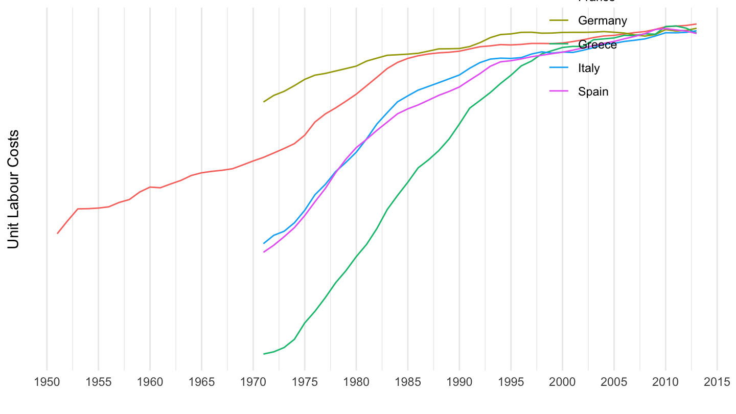
Unit Labour Costs (1995-2012)
Code
ULC_ANN %>%
  filter(SUBJECT == "ULABUL99",
         MEASURE == "ST",
         SECTOR == "01",
         LOCATION %in% c("FRA", "DEU", "ITA", "GRC", "ESP")) %>%
  left_join(ULC_ANN_var$LOCATION, by = "LOCATION") %>%
  year_to_date %>%
  filter(date >= as.Date("1995-01-01")) %>%
  group_by(Location) %>%
  mutate(obsValue = 100*obsValue / obsValue[date == as.Date("2000-01-01")]) %>%
  ggplot() + theme_minimal() + ylab("Unit Labour Costs") + xlab("") +
  geom_line(aes(x = date, y = obsValue, color = Location)) +
  theme(legend.position = c(0.15, 0.8),
        legend.title = element_blank()) +
  scale_x_date(breaks = seq(1920, 2100, 1) %>% paste0("-01-01") %>% as.Date,
               labels = date_format("%Y")) +
  scale_y_log10(breaks = seq(0, 200, 10))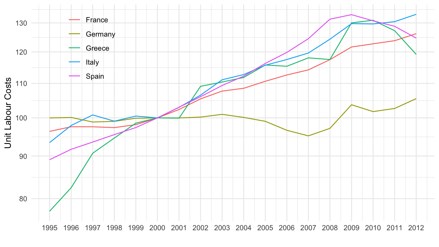
Unit Labour Costs (2000-)
Code
ULC_ANN %>%
  filter(SUBJECT == "ULABUL99",
         MEASURE == "ST",
         SECTOR == "01",
         LOCATION %in% c("FRA", "DEU", "ITA", "GRC", "ESP")) %>%
  left_join(ULC_ANN_var$LOCATION, by = "LOCATION") %>%
  year_to_date %>%
  filter(date >= as.Date("2000-01-01")) %>%
  group_by(Location) %>%
  mutate(obsValue = 100*obsValue / obsValue[date == as.Date("2000-01-01")]) %>%
  ggplot() + theme_minimal() + ylab("Unit Labour Costs") + xlab("") +
  geom_line(aes(x = date, y = obsValue, color = Location)) +
  theme(legend.position = c(0.15, 0.8),
        legend.title = element_blank()) +
  scale_x_date(breaks = seq(1920, 2100, 1) %>% paste0("-01-01") %>% as.Date,
               labels = date_format("%Y")) +
  scale_y_log10(breaks = seq(0, 200, 10))
Labour Income Share (Real ULC)
Total Economy
Code
ULC_ANN %>%
  filter(SUBJECT == "ULAIRU99",
         MEASURE == "ST",
         SECTOR == "01",
         LOCATION %in% c("FRA", "DEU")) %>%
  left_join(ULC_ANN_var$LOCATION, by = "LOCATION") %>%
  year_to_enddate %>%
  ggplot() + theme_minimal() + ylab("Labour Income Share, Real ULC") + xlab("") +
  geom_line(aes(x = date, y = obsValue, color = Location)) +
  scale_color_manual(values = c("#ED2939", "#000000")) +
  theme(legend.position = c(0.8, 0.9),
        legend.title = element_blank()) +
  scale_x_date(breaks = seq(1920, 2100, 5) %>% paste0("-01-01") %>% as.Date,
               labels = date_format("%Y")) +
  scale_y_continuous(breaks = 0.01*seq(0, 100, 5))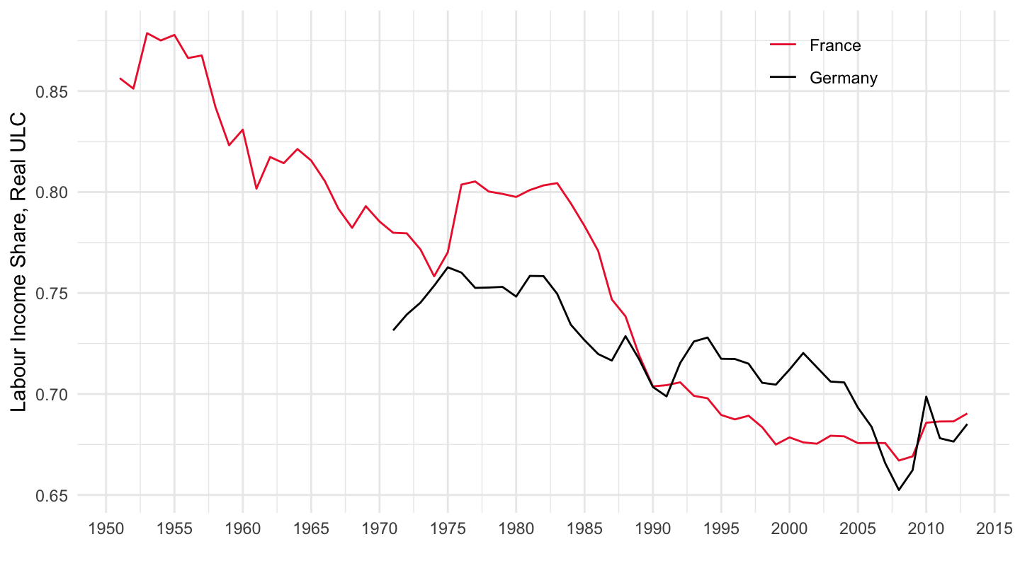
Manufacturing
Code
ULC_ANN %>%
  filter(SUBJECT == "ULAIRU99",
         MEASURE == "ST",
         SECTOR == "02",
         LOCATION %in% c("FRA", "DEU")) %>%
  left_join(ULC_ANN_var$LOCATION, by = "LOCATION") %>%
  year_to_enddate %>%
  ggplot() + theme_minimal() + ylab("Labour Income Share, Real ULC") + xlab("") +
  geom_line(aes(x = date, y = obsValue, color = Location)) +
  scale_color_manual(values = c("#ED2939", "#000000")) +
  theme(legend.position = c(0.8, 0.9),
        legend.title = element_blank()) +
  scale_x_date(breaks = seq(1920, 2100, 5) %>% paste0("-01-01") %>% as.Date,
               labels = date_format("%Y")) +
  scale_y_continuous(breaks = 0.01*seq(0, 100, 2))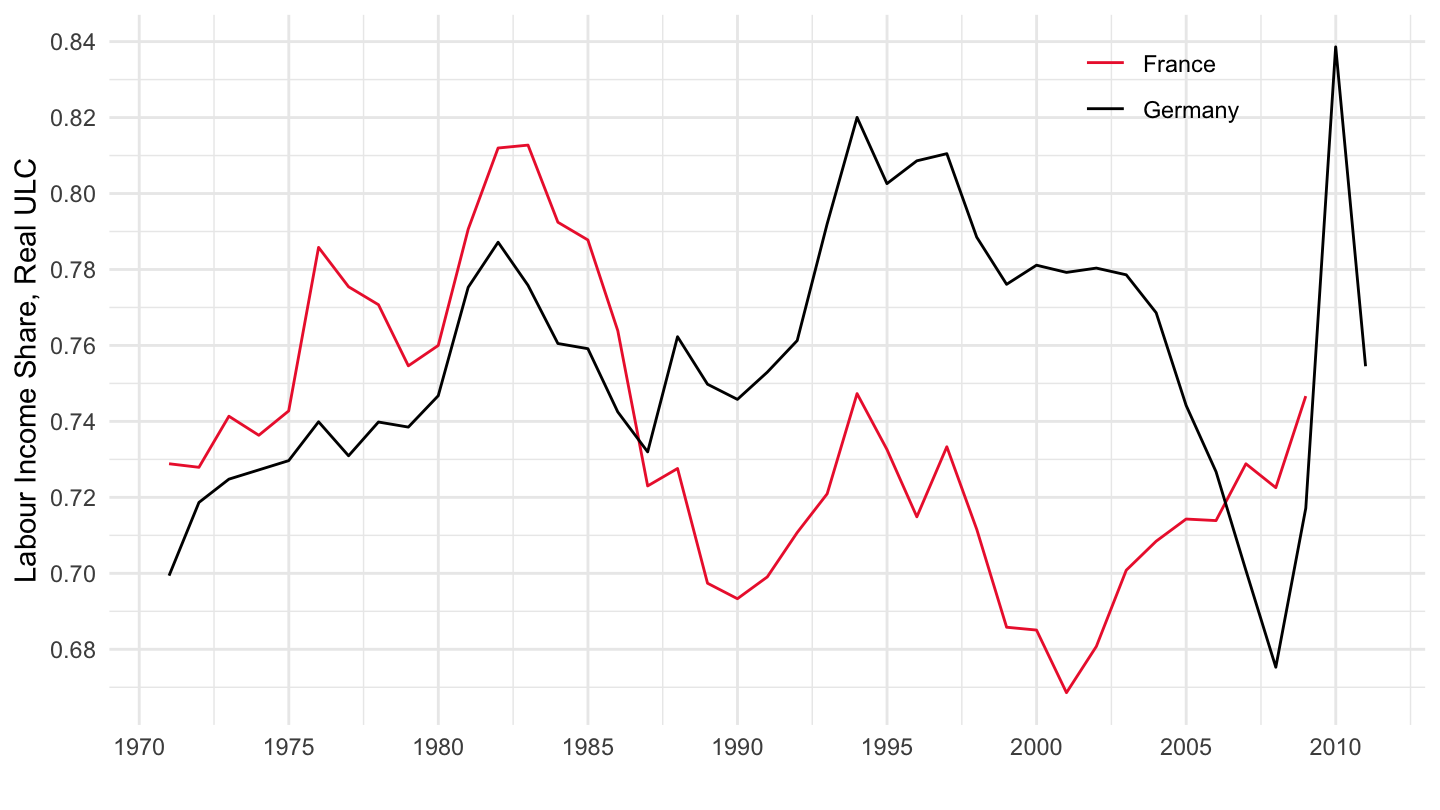
Industry
Code
ULC_ANN %>%
  filter(SUBJECT == "ULAIRU99",
         MEASURE == "ST",
         SECTOR == "03",
         LOCATION %in% c("FRA", "DEU")) %>%
  left_join(ULC_ANN_var$LOCATION, by = "LOCATION") %>%
  year_to_enddate %>%
  ggplot() + theme_minimal() + ylab("Labour Income Share, Real ULC") + xlab("") +
  geom_line(aes(x = date, y = obsValue, color = Location)) +
  scale_color_manual(values = c("#ED2939", "#000000")) +
  theme(legend.position = c(0.8, 0.9),
        legend.title = element_blank()) +
  scale_x_date(breaks = seq(1920, 2100, 5) %>% paste0("-01-01") %>% as.Date,
               labels = date_format("%Y")) +
  scale_y_continuous(breaks = 0.01*seq(0, 100, 2))
Construction
Code
ULC_ANN %>%
  filter(SUBJECT == "ULAIRU99",
         MEASURE == "ST",
         SECTOR == "04",
         LOCATION %in% c("FRA", "DEU")) %>%
  left_join(ULC_ANN_var$LOCATION, by = "LOCATION") %>%
  year_to_enddate %>%
  ggplot() + theme_minimal() + ylab("Labour Income Share, Real ULC") + xlab("") +
  geom_line(aes(x = date, y = obsValue, color = Location)) +
  scale_color_manual(values = c("#ED2939", "#000000")) +
  theme(legend.position = c(0.8, 0.9),
        legend.title = element_blank()) +
  scale_x_date(breaks = seq(1920, 2100, 5) %>% paste0("-01-01") %>% as.Date,
               labels = date_format("%Y")) +
  scale_y_continuous(breaks = 0.01*seq(0, 100, 2))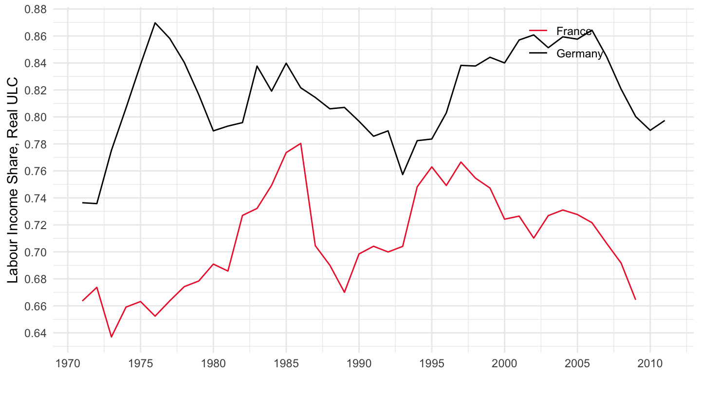
Competitiveness: Unit Labor cost
Total Economy
Code
ULC_ANN %>%
  filter(SUBJECT == "ULABUL99",
         MEASURE == "ST",
         SECTOR == "01",
         LOCATION %in% c("FRA", "DEU")) %>%
  left_join(ULC_ANN_var$LOCATION, by = "LOCATION") %>%
  year_to_date %>%
  filter(year(date) >= 1990) %>%
  arrange(Location) %>%
  ggplot() + geom_line(aes(x = date, y = obsValue, color = Location)) +
  scale_color_manual(values = c("#ED2939", "#000000")) +
  theme_minimal() + ylab("Unit Labour Cost (Total Economy)") + xlab("") +
  scale_x_date(breaks = seq(1920, 2100, 2) %>% paste0("-01-01") %>% as.Date,
               labels = date_format("%Y")) +
  theme(legend.position = c(0.2, 0.9),
        legend.title = element_blank()) +
  scale_y_continuous(breaks = 0.01*seq(0, 100, 5))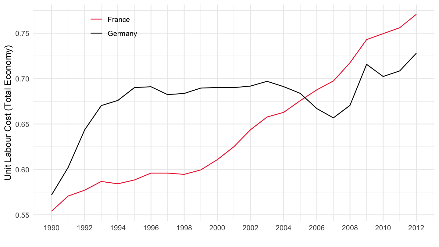
Manufacturing
Code
ULC_ANN %>%
  filter(SUBJECT == "ULABUL99",
         MEASURE == "ST",
         SECTOR == "02",
         LOCATION %in% c("FRA", "DEU")) %>%
  left_join(ULC_ANN_var$LOCATION, by = "LOCATION") %>%
  year_to_date %>%
  filter(year(date) >= 1990) %>%
  arrange(Location) %>%
  ggplot() + geom_line(aes(x = date, y = obsValue, color = Location)) +
  scale_color_manual(values = c("#ED2939", "#000000")) +
  theme_minimal() +
  scale_x_date(breaks = seq(1920, 2100, 2) %>% paste0("-01-01") %>% as.Date,
               labels = date_format("%Y")) +
  theme(legend.position = c(0.8, 0.9),
        legend.title = element_blank()) +
  scale_y_continuous(breaks = 0.01*seq(0, 100, 1)) +
  ylab("Unit Labour Cost (Manufacturing)") + xlab("")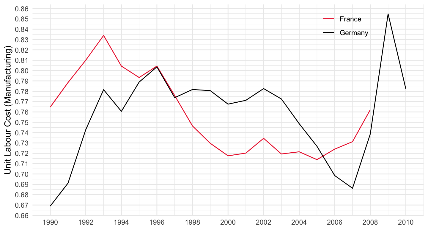
Industry
Code
ULC_ANN %>%
  filter(SUBJECT == "ULABUL99",
         MEASURE == "ST",
         SECTOR == "03",
         LOCATION %in% c("FRA", "DEU")) %>%
  left_join(ULC_ANN_var$LOCATION, by = "LOCATION") %>%
  year_to_date %>%
  filter(year(date) >= 1990) %>%
  arrange(Location) %>%
  ggplot() + geom_line(aes(x = date, y = obsValue, color = Location)) +
  scale_color_manual(values = c("#ED2939", "#000000")) +
  theme_minimal() +
  scale_x_date(breaks = seq(1920, 2100, 2) %>% paste0("-01-01") %>% as.Date,
               labels = date_format("%Y")) +
  theme(legend.position = c(0.8, 0.9),
        legend.title = element_blank()) +
  scale_y_continuous(breaks = 0.01*seq(0, 100, 1)) +
  ylab("Unit Labour Cost (Industry)") + xlab("")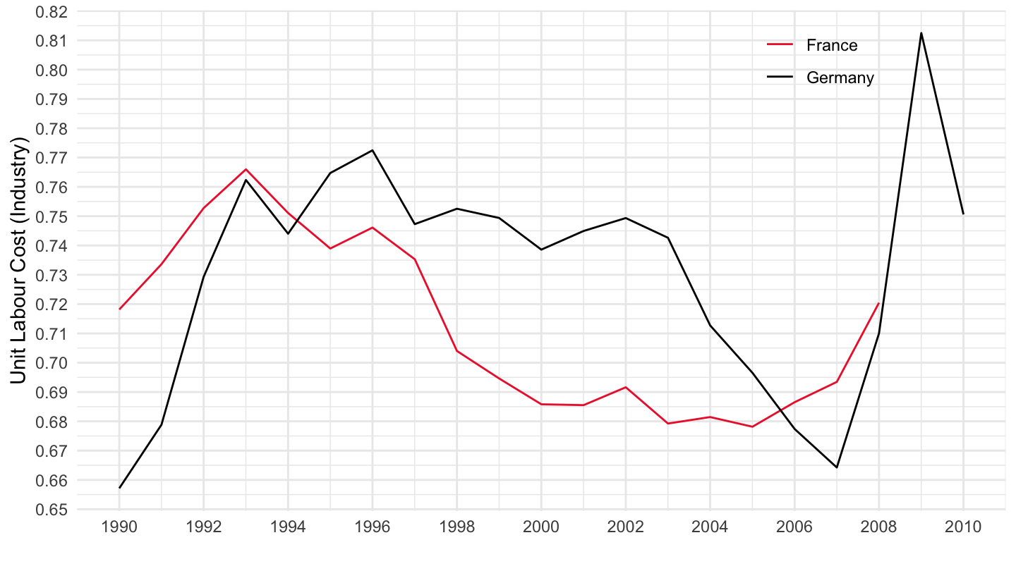
Construction
Code
ULC_ANN %>%
  filter(SUBJECT == "ULABUL99",
         MEASURE == "ST",
         SECTOR == "04",
         LOCATION %in% c("FRA", "DEU")) %>%
  left_join(ULC_ANN_var$LOCATION, by = "LOCATION") %>%
  year_to_date %>%
  filter(year(date) >= 1990) %>%
  arrange(Location) %>%
  ggplot() + geom_line(aes(x = date, y = obsValue, color = Location)) +
  scale_color_manual(values = c("#ED2939", "#000000")) +
  theme_minimal() +
  scale_x_date(breaks = seq(1920, 2100, 2) %>% paste0("-01-01") %>% as.Date,
               labels = date_format("%Y")) +
  theme(legend.position = c(0.8, 0.9),
        legend.title = element_blank()) +
  scale_y_continuous(breaks = 0.01*seq(0, 100, 5)) +
  ylab("Unit Labour Cost (Construction)") + xlab("")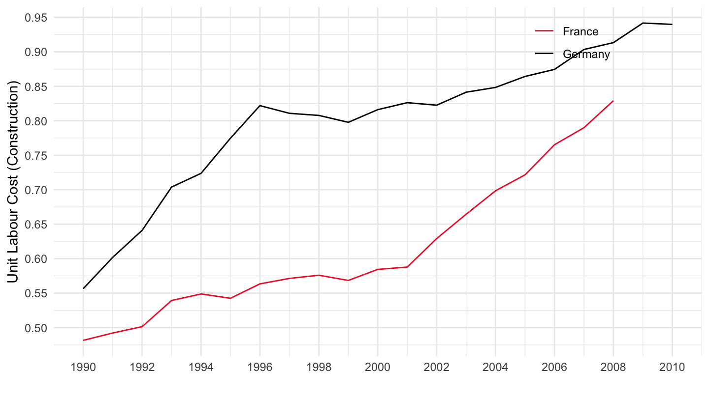
Trade, transport and communication (G_I)
Code
ULC_ANN %>%
  filter(SUBJECT == "ULABUL99",
         MEASURE == "ST",
         SECTOR == "05",
         LOCATION %in% c("FRA", "DEU")) %>%
  left_join(ULC_ANN_var$LOCATION, by = "LOCATION") %>%
  year_to_date %>%
  filter(year(date) >= 1990) %>%
  arrange(Location) %>%
  ggplot() + geom_line(aes(x = date, y = obsValue, color = Location)) +
  scale_color_manual(values = c("#ED2939", "#000000")) +
  theme_minimal() +
  scale_x_date(breaks = seq(1920, 2100, 2) %>% paste0("-01-01") %>% as.Date,
               labels = date_format("%Y")) +
  theme(legend.position = c(0.8, 0.9),
        legend.title = element_blank()) +
  scale_y_continuous(breaks = 0.01*seq(0, 100, 5)) +
  ylab("Unit Labour Cost (Trade, transport and communication") + xlab("")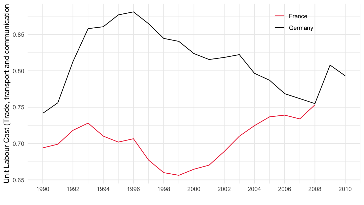
Financial and business services
Code
ULC_ANN %>%
  filter(SUBJECT == "ULABUL99",
         MEASURE == "ST",
         SECTOR == "06",
         LOCATION %in% c("FRA", "DEU")) %>%
  left_join(ULC_ANN_var$LOCATION, by = "LOCATION") %>%
  year_to_date %>%
  filter(year(date) >= 1990) %>%
  arrange(Location) %>%
  ggplot() + geom_line(aes(x = date, y = obsValue, color = Location)) +
  scale_color_manual(values = c("#ED2939", "#000000")) +
  theme_minimal() +
  scale_x_date(breaks = seq(1920, 2100, 2) %>% paste0("-01-01") %>% as.Date,
               labels = date_format("%Y")) +
  theme(legend.position = c(0.2, 0.9),
        legend.title = element_blank()) +
  scale_y_continuous(breaks = 0.01*seq(0, 100, 5)) +
  ylab("Unit Labour Cost (Financial and business services)") + xlab("")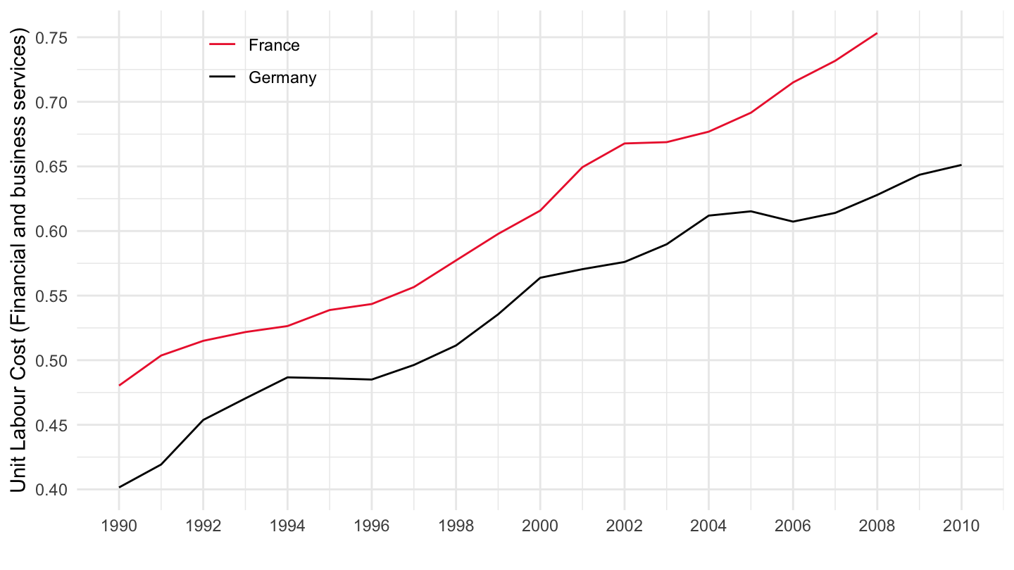
Market services
Code
ULC_ANN %>%
  filter(SUBJECT == "ULABUL99",
         MEASURE == "ST",
         SECTOR == "07",
         LOCATION %in% c("FRA", "DEU")) %>%
  left_join(ULC_ANN_var$LOCATION, by = "LOCATION") %>%
  year_to_date %>%
  filter(year(date) >= 1990) %>%
  arrange(Location) %>%
  ggplot() + geom_line(aes(x = date, y = obsValue, color = Location)) +
  scale_color_manual(values = c("#ED2939", "#000000")) +
  theme_minimal() +
  scale_x_date(breaks = seq(1920, 2100, 2) %>% paste0("-01-01") %>% as.Date,
               labels = date_format("%Y")) +
  theme(legend.position = c(0.2, 0.9),
        legend.title = element_blank()) +
  scale_y_continuous(breaks = 0.01*seq(0, 100, 5)) +
  ylab("Unit Labour Cost (Market services)") + xlab("")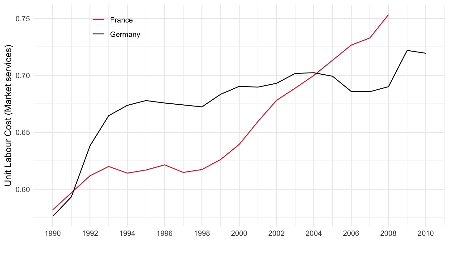
Business sector excl. Agriculture
Code
ULC_ANN %>%
  filter(SUBJECT == "ULABUL99",
         MEASURE == "ST",
         SECTOR == "08",
         LOCATION %in% c("FRA", "DEU")) %>%
  left_join(ULC_ANN_var$LOCATION, by = "LOCATION") %>%
  year_to_date %>%
  filter(year(date) >= 1990) %>%
  arrange(Location) %>%
  ggplot() + geom_line(aes(x = date, y = obsValue, color = Location)) +
  scale_color_manual(values = c("#ED2939", "#000000")) +
  theme_minimal() +
  scale_x_date(breaks = seq(1920, 2100, 2) %>% paste0("-01-01") %>% as.Date,
               labels = date_format("%Y")) +
  theme(legend.position = c(0.2, 0.9),
        legend.title = element_blank()) +
  scale_y_continuous(breaks = 0.01*seq(0, 100, 5)) +
  ylab("Unit Labour Cost (Business sector excl. Agriculture)") + xlab("")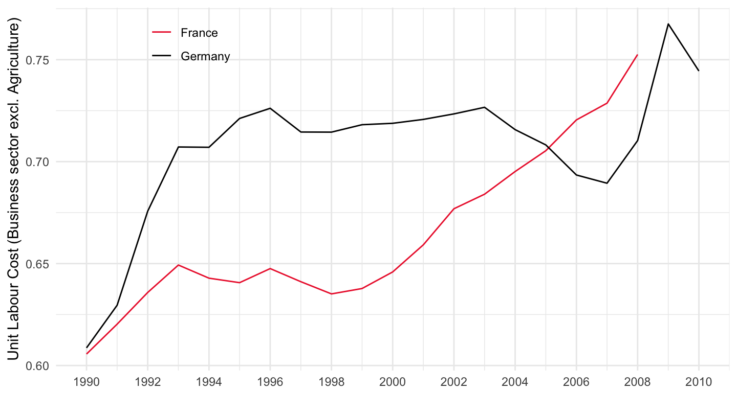
Competitiveness: Exchange Rate Adjusted ULC
Total Economy
Code
ULC_ANN %>%
  filter(SUBJECT == "ULAIEU99",
         MEASURE == "ST",
         SECTOR == "01",
         LOCATION %in% c("FRA", "DEU")) %>%
  left_join(ULC_ANN_var$LOCATION, by = "LOCATION") %>%
  year_to_date %>%
  filter(year(date) >= 1990) %>%
  arrange(Location) %>%
  ggplot() + geom_line(aes(x = date, y = obsValue, color = Location)) +
  scale_color_manual(values = c("#ED2939", "#000000")) +
  theme_minimal() +
  scale_x_date(breaks = seq(1920, 2100, 2) %>% paste0("-01-01") %>% as.Date,
               labels = date_format("%Y")) +
  theme(legend.position = c(0.2, 0.9),
        legend.title = element_blank()) +
  scale_y_continuous(breaks = 0.01*seq(0, 100, 5)) +
  ylab("Exchange Rate Adjusted ULC (Total Economy)") + xlab("")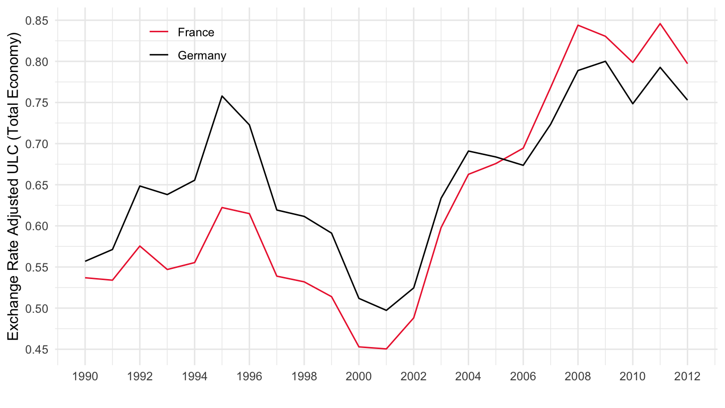
Manufacturing
Code
ULC_ANN %>%
  filter(SUBJECT == "ULAIEU99",
         MEASURE == "ST",
         SECTOR == "02",
         LOCATION %in% c("FRA", "DEU")) %>%
  left_join(ULC_ANN_var$LOCATION, by = "LOCATION") %>%
  year_to_date %>%
  filter(year(date) >= 1990) %>%
  arrange(Location) %>%
  ggplot() + geom_line(aes(x = date, y = obsValue, color = Location)) +
  scale_color_manual(values = c("#ED2939", "#000000")) +
  theme_minimal() +
  scale_x_date(breaks = seq(1920, 2100, 2) %>% paste0("-01-01") %>% as.Date,
               labels = date_format("%Y")) +
  theme(legend.position = c(0.8, 0.9),
        legend.title = element_blank()) +
  scale_y_continuous(breaks = 0.01*seq(0, 100, 1)) +
  ylab("Exchange Rate Adjusted ULC (Manufacturing)") + xlab("")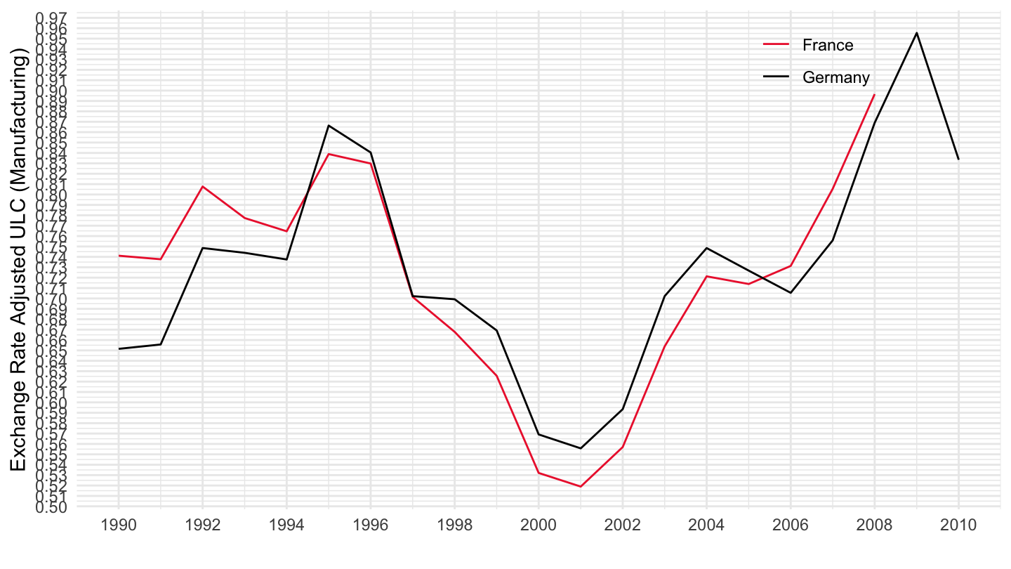
Industry
Code
ULC_ANN %>%
  filter(SUBJECT == "ULAIEU99",
         MEASURE == "ST",
         SECTOR == "03",
         LOCATION %in% c("FRA", "DEU")) %>%
  left_join(ULC_ANN_var$LOCATION, by = "LOCATION") %>%
  year_to_date %>%
  filter(year(date) >= 1990) %>%
  arrange(Location) %>%
  ggplot() + geom_line(aes(x = date, y = obsValue, color = Location)) +
  scale_color_manual(values = c("#ED2939", "#000000")) +
  theme_minimal() +
  scale_x_date(breaks = seq(1920, 2100, 2) %>% paste0("-01-01") %>% as.Date,
               labels = date_format("%Y")) +
  theme(legend.position = c(0.8, 0.9),
        legend.title = element_blank()) +
  scale_y_continuous(breaks = 0.01*seq(0, 100, 1)) +
  ylab("Exchange Rate Adjusted ULC (Industry)") + xlab("")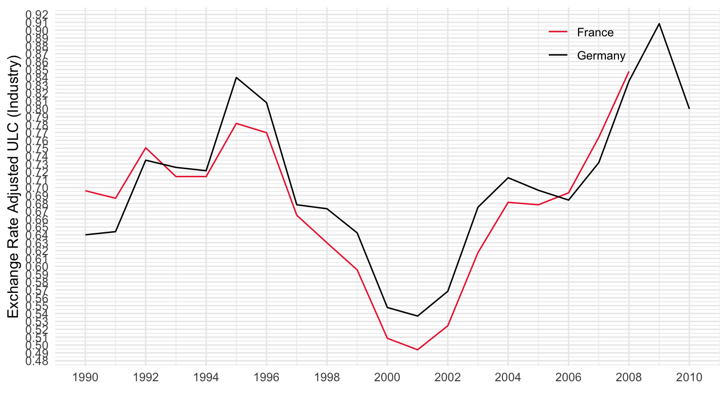
Construction
Code
ULC_ANN %>%
  filter(SUBJECT == "ULAIEU99",
         MEASURE == "ST",
         SECTOR == "04",
         LOCATION %in% c("FRA", "DEU")) %>%
  left_join(ULC_ANN_var$LOCATION, by = "LOCATION") %>%
  year_to_date %>%
  filter(year(date) >= 1990) %>%
  arrange(Location) %>%
  ggplot() + geom_line(aes(x = date, y = obsValue, color = Location)) +
  scale_color_manual(values = c("#ED2939", "#000000")) +
  theme_minimal() +
  scale_x_date(breaks = seq(1920, 2100, 2) %>% paste0("-01-01") %>% as.Date,
               labels = date_format("%Y")) +
  theme(legend.position = c(0.8, 0.9),
        legend.title = element_blank()) +
  scale_y_continuous(breaks = 0.01*seq(0, 100, 5)) +
  ylab("Exchange Rate Adjusted ULC (Construction)") + xlab("")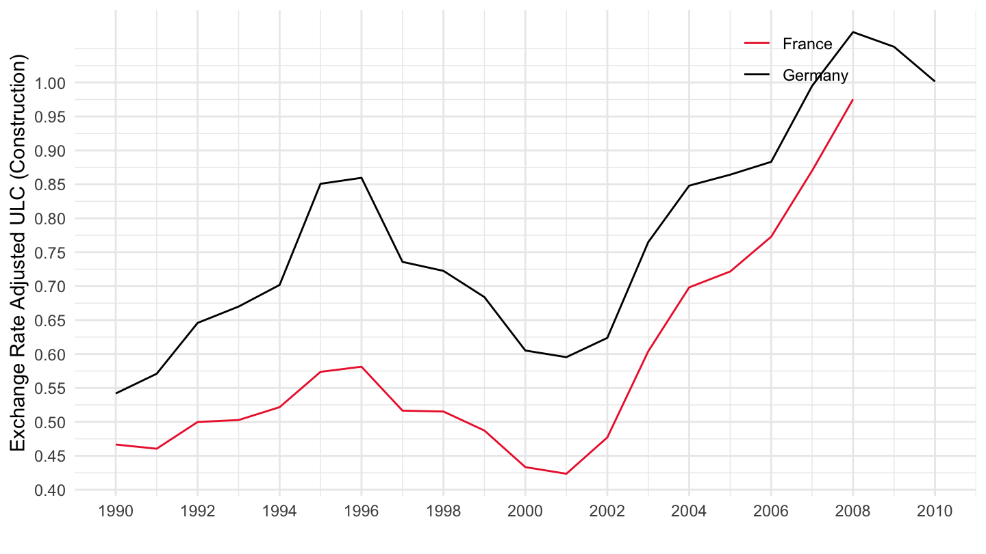
Trade, transport and communication (G_I)
Code
ULC_ANN %>%
  filter(SUBJECT == "ULAIEU99",
         MEASURE == "ST",
         SECTOR == "05",
         LOCATION %in% c("FRA", "DEU")) %>%
  left_join(ULC_ANN_var$LOCATION, by = "LOCATION") %>%
  year_to_date %>%
  filter(year(date) >= 1990) %>%
  arrange(Location) %>%
  ggplot() + geom_line(aes(x = date, y = obsValue, color = Location)) +
  scale_color_manual(values = c("#ED2939", "#000000")) +
  theme_minimal() +
  scale_x_date(breaks = seq(1920, 2100, 2) %>% paste0("-01-01") %>% as.Date,
               labels = date_format("%Y")) +
  theme(legend.position = c(0.8, 0.9),
        legend.title = element_blank()) +
  scale_y_continuous(breaks = 0.01*seq(0, 100, 5)) +
  ylab("Exchange Rate Adjusted ULC (Trade, transport and communication)") + xlab("")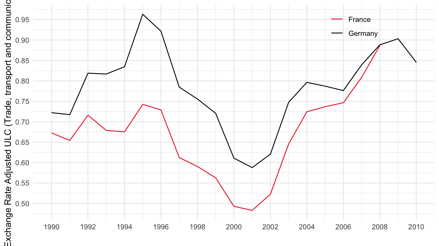
Financial and business services
Code
ULC_ANN %>%
  filter(SUBJECT == "ULAIEU99",
         MEASURE == "ST",
         SECTOR == "06",
         LOCATION %in% c("FRA", "DEU")) %>%
  left_join(ULC_ANN_var$LOCATION, by = "LOCATION") %>%
  year_to_date %>%
  filter(year(date) >= 1990) %>%
  arrange(Location) %>%
  ggplot() + geom_line(aes(x = date, y = obsValue, color = Location)) +
  scale_color_manual(values = c("#ED2939", "#000000")) +
  theme_minimal() +
  scale_x_date(breaks = seq(1920, 2100, 2) %>% paste0("-01-01") %>% as.Date,
               labels = date_format("%Y")) +
  theme(legend.position = c(0.2, 0.9),
        legend.title = element_blank()) +
  scale_y_continuous(breaks = 0.01*seq(0, 100, 5)) +
  ylab("Exchange Rate Adjusted ULC (Financial and business services)") + xlab("")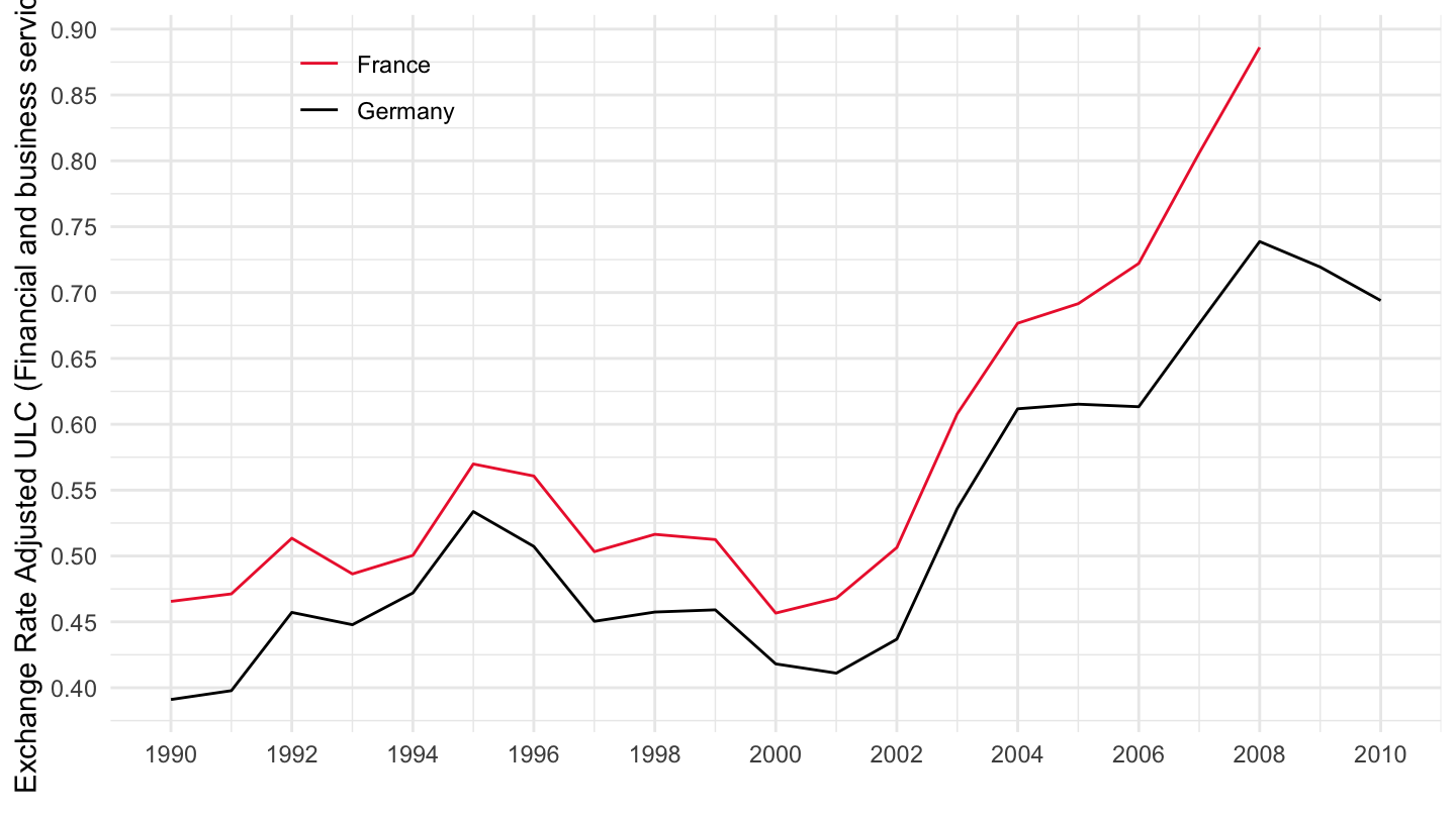
Market services
Code
ULC_ANN %>%
  filter(SUBJECT == "ULAIEU99",
         MEASURE == "ST",
         SECTOR == "07",
         LOCATION %in% c("FRA", "DEU")) %>%
  left_join(ULC_ANN_var$LOCATION, by = "LOCATION") %>%
  year_to_date %>%
  filter(year(date) >= 1990) %>%
  arrange(Location) %>%
  ggplot() + geom_line(aes(x = date, y = obsValue, color = Location)) +
  scale_color_manual(values = c("#ED2939", "#000000")) +
  theme_minimal() +
  scale_x_date(breaks = seq(1920, 2100, 2) %>% paste0("-01-01") %>% as.Date,
               labels = date_format("%Y")) +
  theme(legend.position = c(0.2, 0.9),
        legend.title = element_blank()) +
  scale_y_continuous(breaks = 0.01*seq(0, 100, 5)) +
  ylab("Exchange Rate Adjusted ULC (Market services)") + xlab("")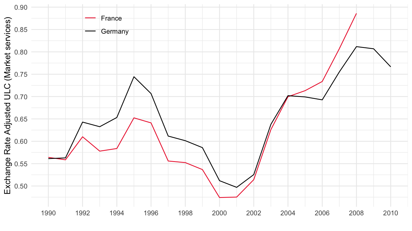
Business sector excl. Agriculture
Code
ULC_ANN %>%
  filter(SUBJECT == "ULAIEU99",
         MEASURE == "ST",
         SECTOR == "08",
         LOCATION %in% c("FRA", "DEU")) %>%
  left_join(ULC_ANN_var$LOCATION, by = "LOCATION") %>%
  year_to_date %>%
  filter(year(date) >= 1990) %>%
  arrange(Location) %>%
  ggplot() + geom_line(aes(x = date, y = obsValue, color = Location)) +
  scale_color_manual(values = c("#ED2939", "#000000")) +
  theme_minimal() +
  scale_x_date(breaks = seq(1920, 2100, 2) %>% paste0("-01-01") %>% as.Date,
               labels = date_format("%Y")) +
  theme(legend.position = c(0.2, 0.9),
        legend.title = element_blank()) +
  scale_y_continuous(breaks = 0.01*seq(0, 100, 5)) +
  ylab("Exchange Rate Adjusted ULC (Business sector excl. Agriculture)") + xlab("")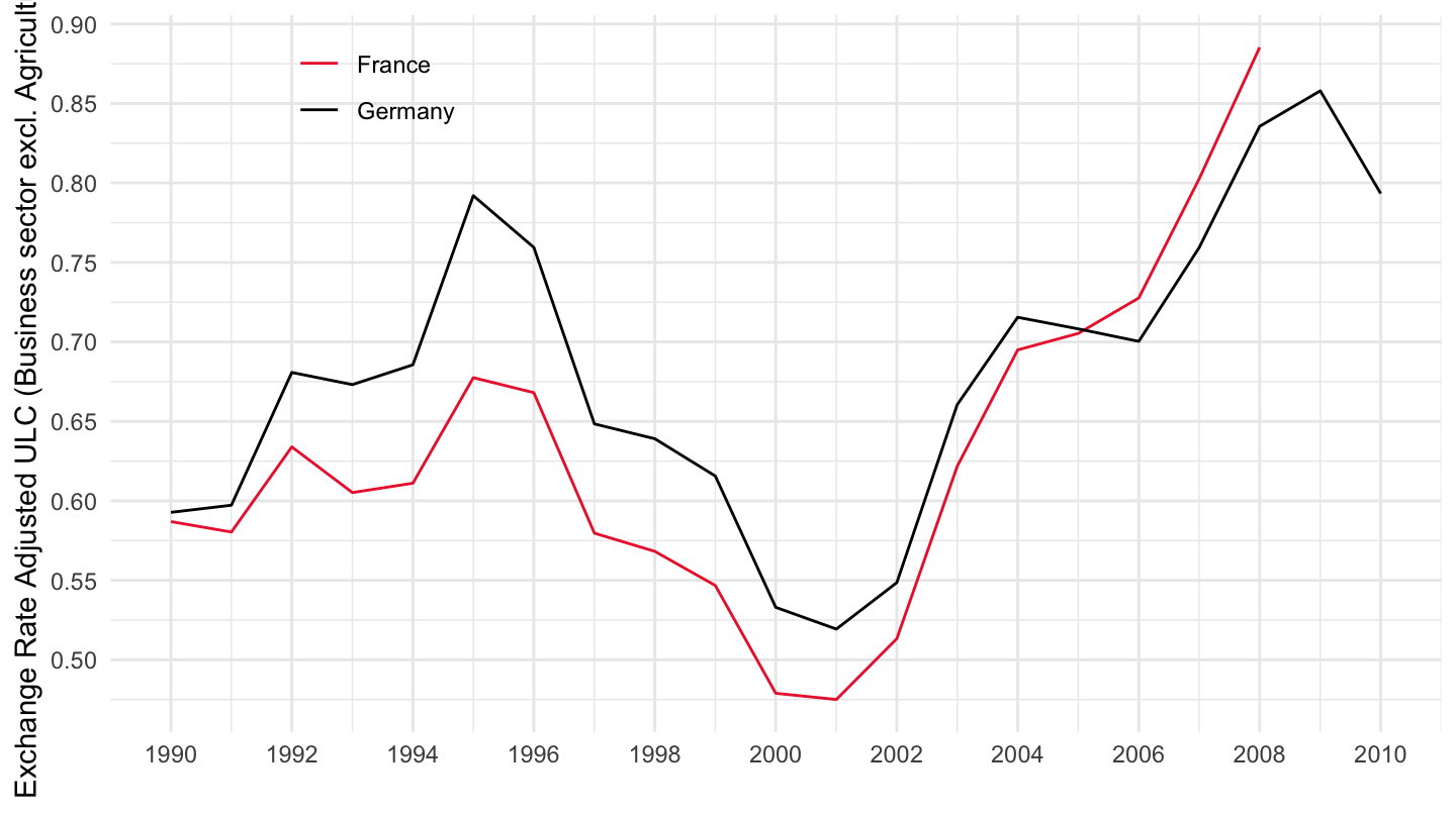
Competitiveness: Labour Income Share (Real ULC)
Total Economy
Code
ULC_ANN %>%
  filter(SUBJECT == "ULAIRU99",
         MEASURE == "ST",
         SECTOR == "01",
         LOCATION %in% c("FRA", "DEU")) %>%
  left_join(ULC_ANN_var$LOCATION, by = "LOCATION") %>%
  year_to_date %>%
  filter(year(date) >= 1990) %>%
  arrange(Location) %>%
  ggplot() + geom_line(aes(x = date, y = obsValue, color = Location)) +
  scale_color_manual(values = c("#ED2939", "#000000")) +
  theme_minimal() +
  scale_x_date(breaks = seq(1920, 2100, 2) %>% paste0("-01-01") %>% as.Date,
               labels = date_format("%Y")) +
  theme(legend.position = c(0.8, 0.9),
        legend.title = element_blank()) +
  scale_y_continuous(breaks = 0.01*seq(0, 100, 1)) +
  ylab("Labour Income Share (Real ULC) (Total Economy)") + xlab("")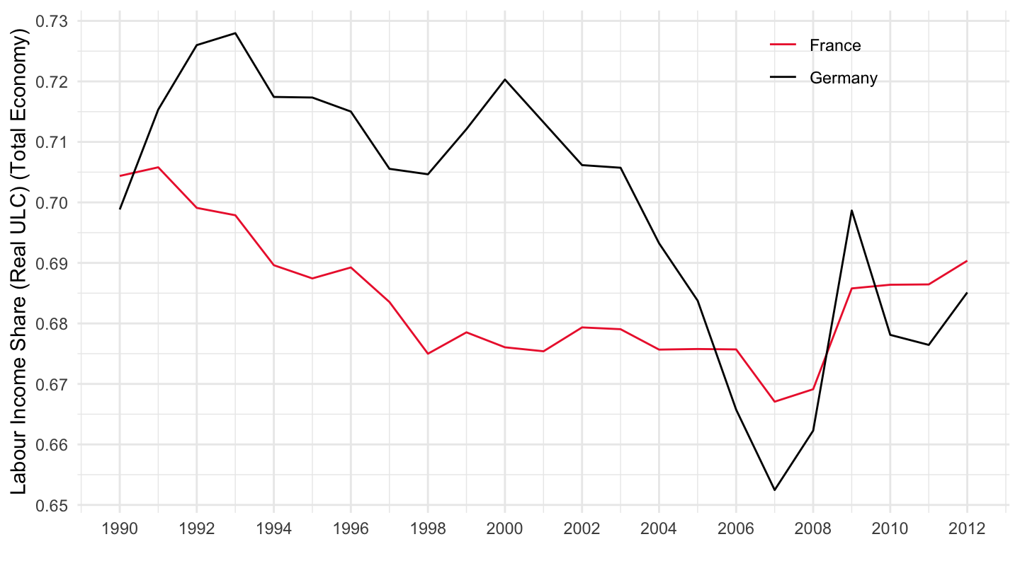
Manufacturing
Code
ULC_ANN %>%
  filter(SUBJECT == "ULAIRU99",
         MEASURE == "ST",
         SECTOR == "02",
         LOCATION %in% c("FRA", "DEU")) %>%
  left_join(ULC_ANN_var$LOCATION, by = "LOCATION") %>%
  year_to_date %>%
  filter(year(date) >= 1990) %>%
  arrange(Location) %>%
  ggplot() + geom_line(aes(x = date, y = obsValue, color = Location)) +
  scale_color_manual(values = c("#ED2939", "#000000")) +
  theme_minimal() +
  scale_x_date(breaks = seq(1920, 2100, 2) %>% paste0("-01-01") %>% as.Date,
               labels = date_format("%Y")) +
  theme(legend.position = c(0.8, 0.9),
        legend.title = element_blank()) +
  scale_y_continuous(breaks = 0.01*seq(0, 100, 1)) +
  ylab("Labour Income Share (Real ULC) (Manufacturing)") + xlab("")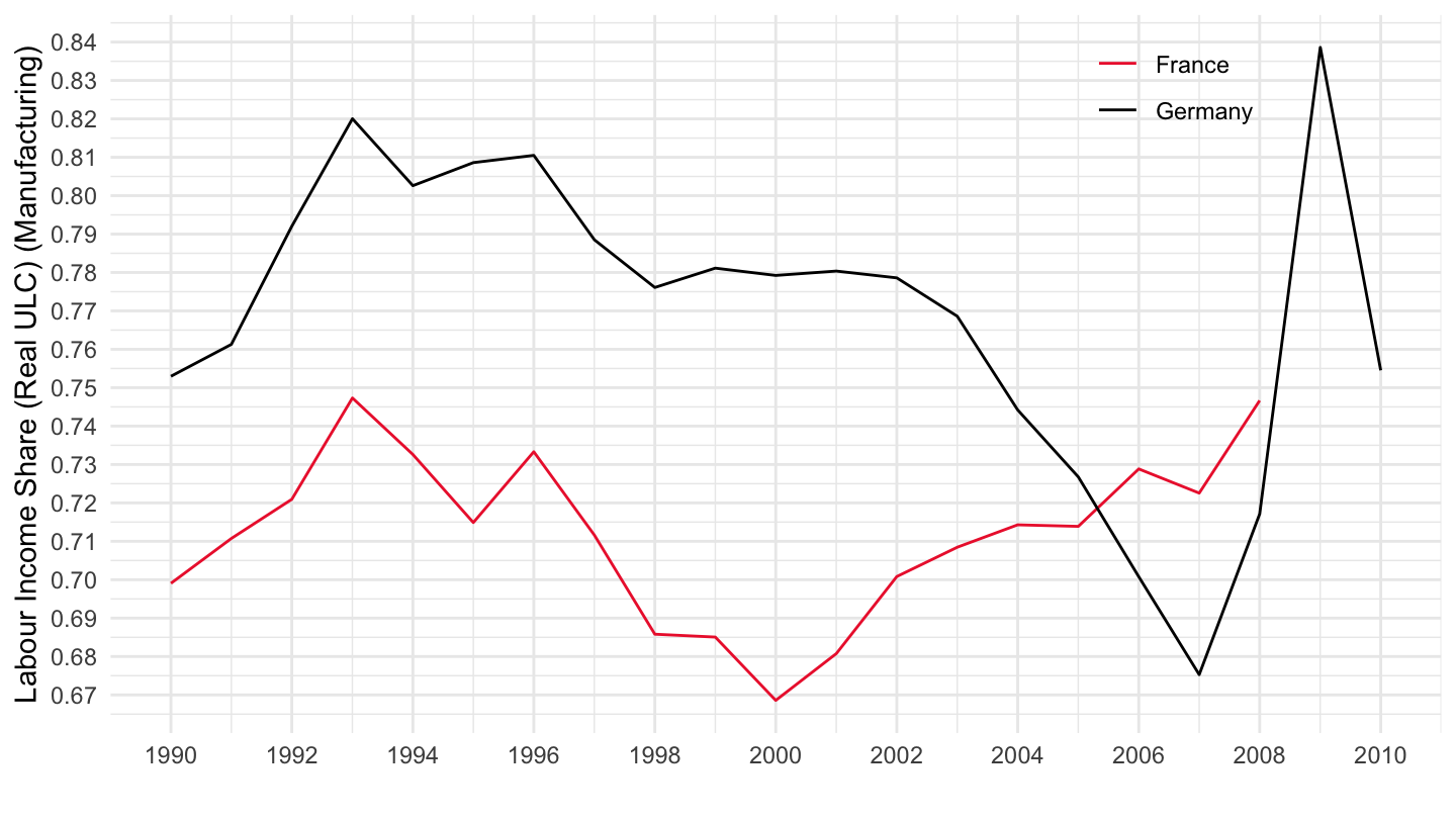
Industry
Code
ULC_ANN %>%
  filter(SUBJECT == "ULAIRU99",
         MEASURE == "ST",
         SECTOR == "03",
         LOCATION %in% c("FRA", "DEU")) %>%
  left_join(ULC_ANN_var$LOCATION, by = "LOCATION") %>%
  year_to_date %>%
  filter(year(date) >= 1990) %>%
  arrange(Location) %>%
  ggplot() + geom_line(aes(x = date, y = obsValue, color = Location)) +
  scale_color_manual(values = c("#ED2939", "#000000")) +
  theme_minimal() +
  scale_x_date(breaks = seq(1920, 2100, 2) %>% paste0("-01-01") %>% as.Date,
               labels = date_format("%Y")) +
  theme(legend.position = c(0.8, 0.9),
        legend.title = element_blank()) +
  scale_y_continuous(breaks = 0.01*seq(0, 100, 1)) +
  ylab("Labour Income Share (Real ULC) (Industry)") + xlab("")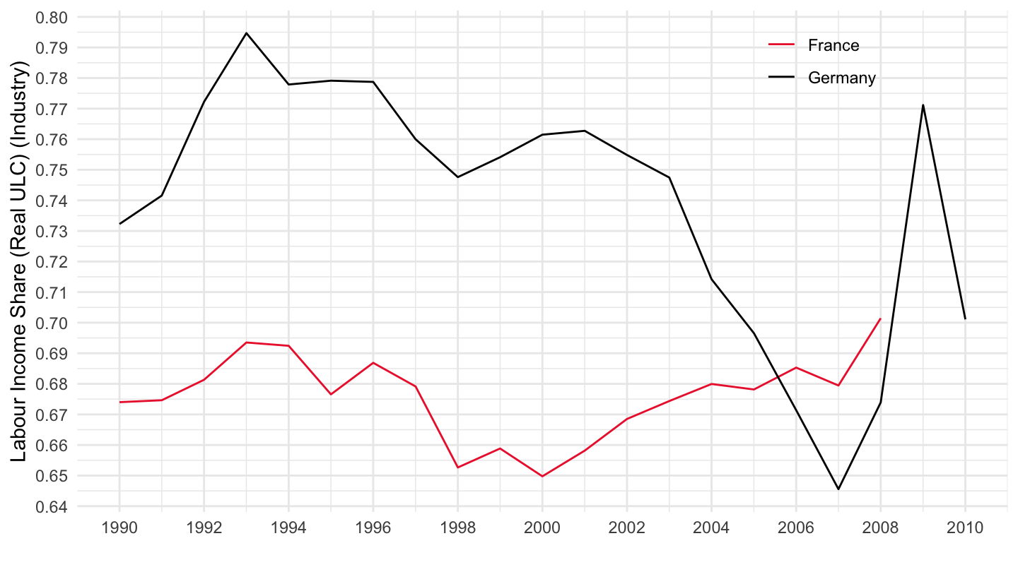
Construction
Code
ULC_ANN %>%
  filter(SUBJECT == "ULAIRU99",
         MEASURE == "ST",
         SECTOR == "04",
         LOCATION %in% c("FRA", "DEU")) %>%
  left_join(ULC_ANN_var$LOCATION, by = "LOCATION") %>%
  year_to_date %>%
  filter(year(date) >= 1990) %>%
  arrange(Location) %>%
  ggplot() + geom_line(aes(x = date, y = obsValue, color = Location)) +
  scale_color_manual(values = c("#ED2939", "#000000")) +
  theme_minimal() +
  scale_x_date(breaks = seq(1920, 2100, 2) %>% paste0("-01-01") %>% as.Date,
               labels = date_format("%Y")) +
  theme(legend.position = c(0.8, 0.9),
        legend.title = element_blank()) +
  scale_y_continuous(breaks = 0.01*seq(0, 100, 5)) +
  ylab("Labour Income Share (Real ULC) (Construction)") + xlab("")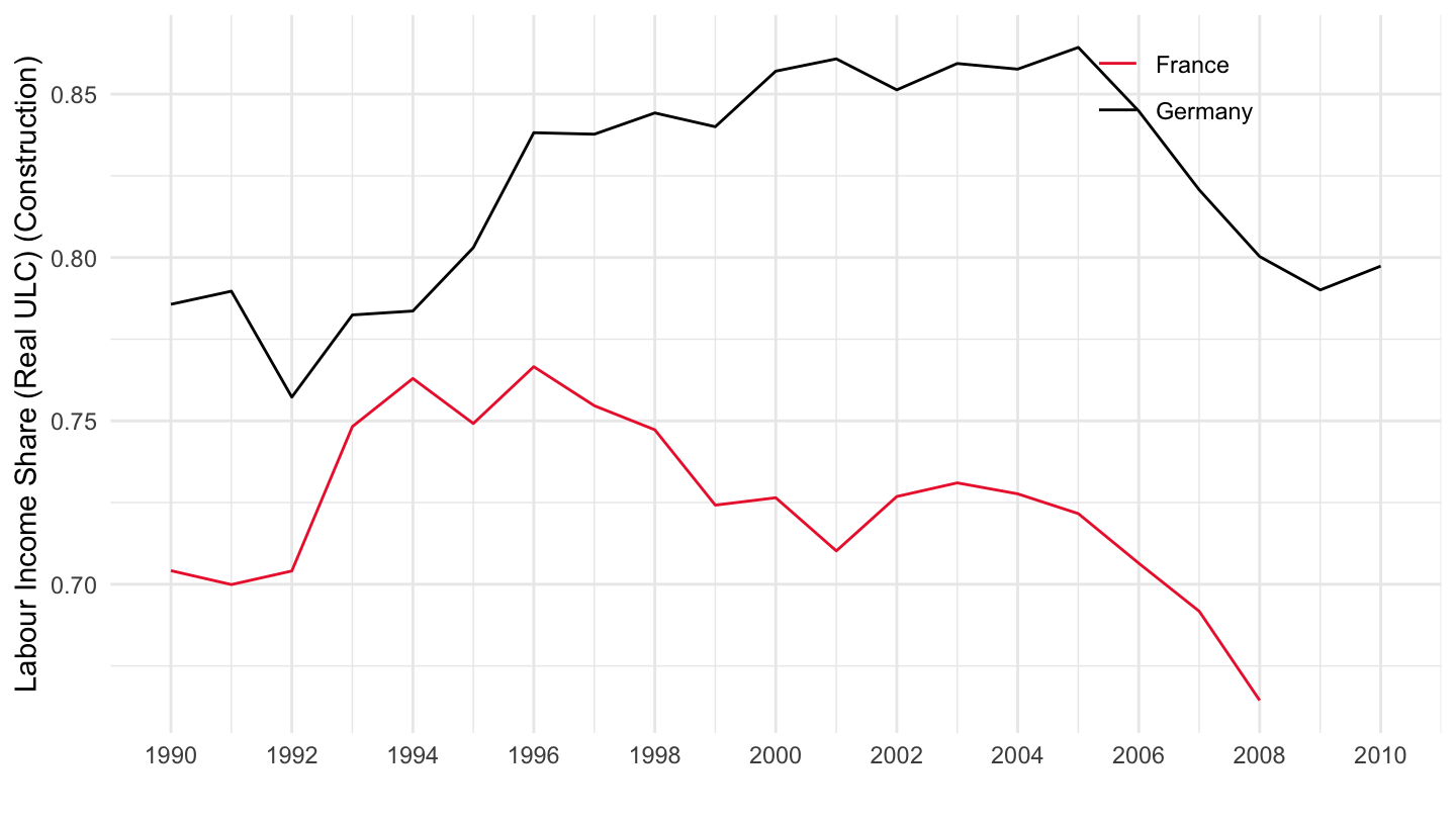
Trade, transport and communication (G_I)
Code
ULC_ANN %>%
  filter(SUBJECT == "ULAIRU99",
         MEASURE == "ST",
         SECTOR == "05",
         LOCATION %in% c("FRA", "DEU")) %>%
  left_join(ULC_ANN_var$LOCATION, by = "LOCATION") %>%
  year_to_date %>%
  filter(year(date) >= 1990) %>%
  arrange(Location) %>%
  ggplot() + geom_line(aes(x = date, y = obsValue, color = Location)) +
  scale_color_manual(values = c("#ED2939", "#000000")) +
  theme_minimal() +
  scale_x_date(breaks = seq(1920, 2100, 2) %>% paste0("-01-01") %>% as.Date,
               labels = date_format("%Y")) +
  theme(legend.position = c(0.8, 0.9),
        legend.title = element_blank()) +
  scale_y_continuous(breaks = 0.01*seq(0, 100, 5)) +
  ylab("Labour Income Share (Real ULC) (Trade, transport and communication)") + xlab("")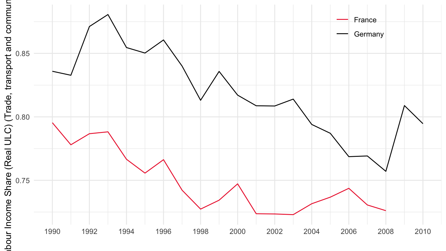
Financial and business services
Code
ULC_ANN %>%
  filter(SUBJECT == "ULAIRU99",
         MEASURE == "ST",
         SECTOR == "06",
         LOCATION %in% c("FRA", "DEU")) %>%
  left_join(ULC_ANN_var$LOCATION, by = "LOCATION") %>%
  year_to_date %>%
  filter(year(date) >= 1990) %>%
  arrange(Location) %>%
  ggplot() + geom_line(aes(x = date, y = obsValue, color = Location)) +
  scale_color_manual(values = c("#ED2939", "#000000")) +
  theme_minimal() +
  scale_x_date(breaks = seq(1920, 2100, 2) %>% paste0("-01-01") %>% as.Date,
               labels = date_format("%Y")) +
  theme(legend.position = c(0.2, 0.9),
        legend.title = element_blank()) +
  scale_y_continuous(breaks = 0.01*seq(0, 100, 5)) +
  ylab("Labour Income Share (Real ULC) (Financial and business services)") + xlab("")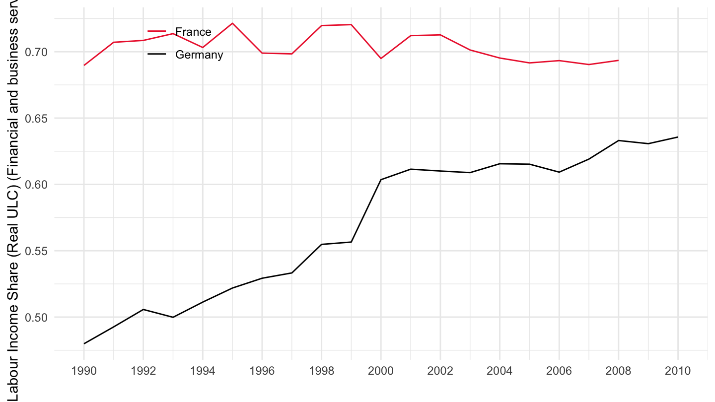
Market services
Code
ULC_ANN %>%
  filter(SUBJECT == "ULAIRU99",
         MEASURE == "ST",
         SECTOR == "07",
         LOCATION %in% c("FRA", "DEU")) %>%
  left_join(ULC_ANN_var$LOCATION, by = "LOCATION") %>%
  year_to_date %>%
  filter(year(date) >= 1990) %>%
  arrange(Location) %>%
  ggplot() + geom_line(aes(x = date, y = obsValue, color = Location)) +
  scale_color_manual(values = c("#ED2939", "#000000")) +
  theme_minimal() +
  scale_x_date(breaks = seq(1920, 2100, 2) %>% paste0("-01-01") %>% as.Date,
               labels = date_format("%Y")) +
  theme(legend.position = c(0.2, 0.9),
        legend.title = element_blank()) +
  scale_y_continuous(breaks = 0.01*seq(0, 100, 5)) +
  ylab("Labour Income Share (Real ULC) (Market services)") + xlab("")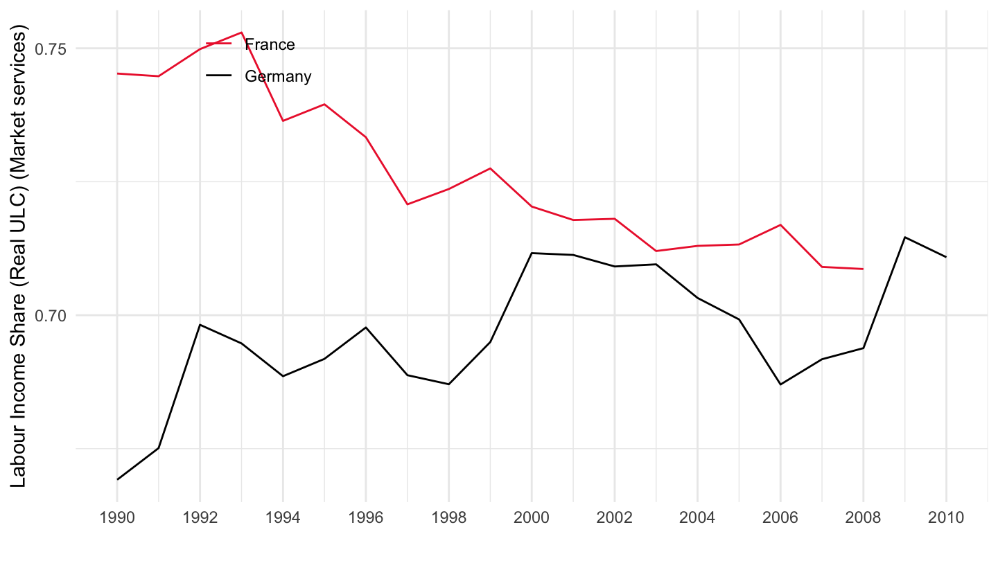
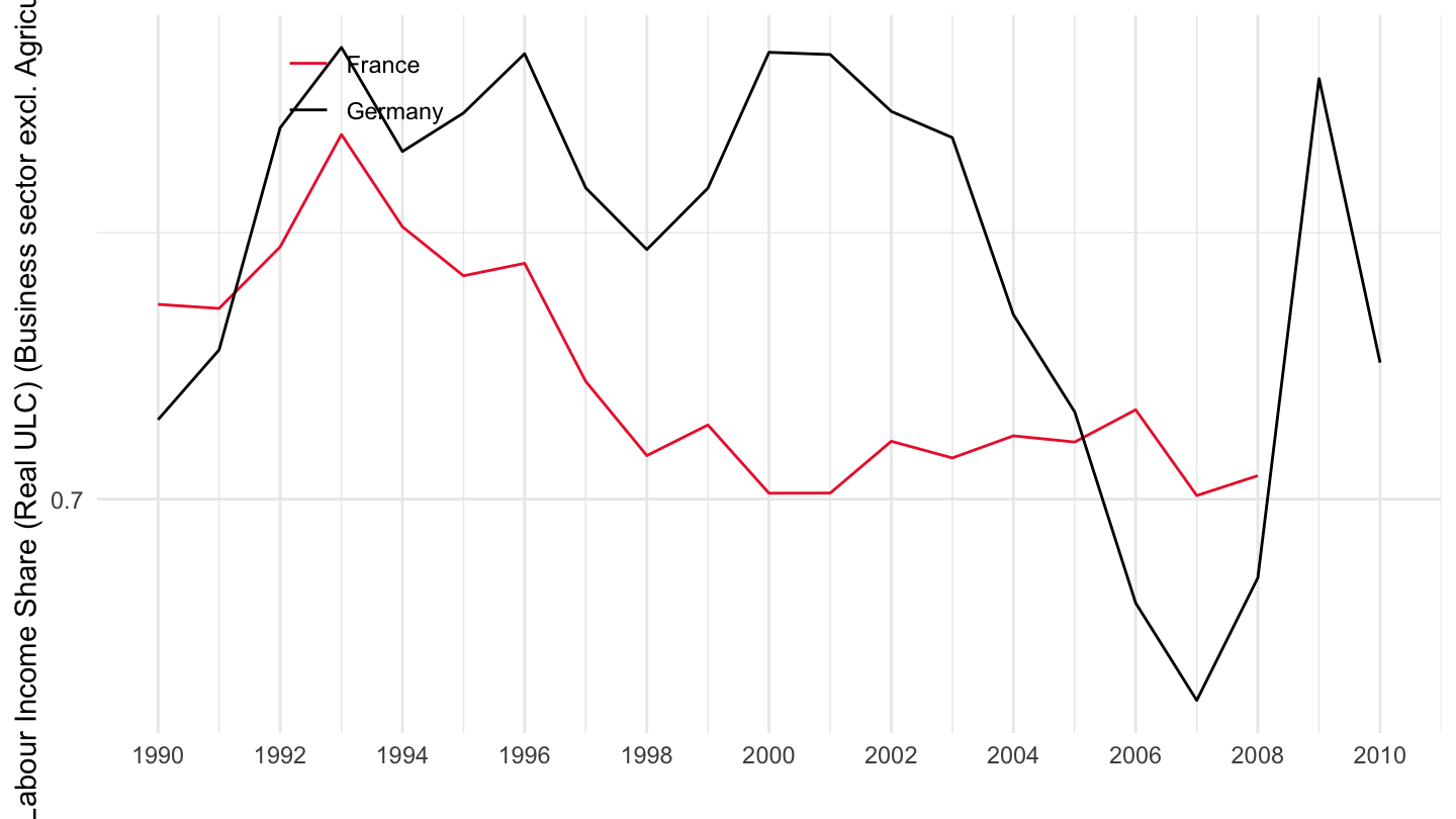
Business sector excl. Agriculture
Code
ULC_ANN %>%
  filter(SUBJECT == "ULAIRU99",
         MEASURE == "ST",
         SECTOR == "08",
         LOCATION %in% c("FRA", "DEU")) %>%
  left_join(ULC_ANN_var$LOCATION, by = "LOCATION") %>%
  year_to_date %>%
  filter(year(date) >= 1990) %>%
  arrange(Location) %>%
  ggplot() + geom_line(aes(x = date, y = obsValue, color = Location)) +
  scale_color_manual(values = c("#ED2939", "#000000")) +
  theme_minimal() +
  scale_x_date(breaks = seq(1920, 2100, 2) %>% paste0("-01-01") %>% as.Date,
               labels = date_format("%Y")) +
  theme(legend.position = c(0.2, 0.9),
        legend.title = element_blank()) +
  scale_y_continuous(breaks = 0.01*seq(0, 100, 5)) +
  ylab("Labour Income Share (Real ULC) (Business sector excl. Agriculture)") + xlab("")