
Last observation: Q2 2023 (N = 1034) · 2022 (N = 1136)
First observation: 1960 (N = 159) · Q1 1960 (N = 153)
Last data update: 02 août 2026, 09:06
Last compile: 09 oct. 2026, 23:40
QNA |>
  filter(FREQUENCY == "A") |>
  left_join(QNA_var$MEASURE, by = "MEASURE") |>
  group_by(MEASURE, Measure) |>
  summarise(Nobs = n()) |>
  arrange(-Nobs) |>
print_table_conditional()| MEASURE | Measure | Nobs |
|---|---|---|
| CQR | National currency, current prices, quarterly levels | 4034 |
| CQRSA | National currency, current prices, quarterly levels, seasonally adjusted | 3919 |
| LNBQRSA | National currency, chained volume estimates, national reference year, quarterly levels, seasonally adjusted | 3854 |
| LNBQR | National currency, chained volume estimates, national reference year, quarterly levels | 3663 |
| CPCARSA | US dollars, current prices, current PPPs, annual levels, seasonally adjusted | 2738 |
| VPVOBARSA | US dollars, volume estimates, fixed PPPs, OECD reference year, annual levels, seasonally adjusted | 2736 |
| GPSA | Growth rate based on seasonally adjusted volume data, percentage change on the previous quarter | 2629 |
| GYSA | Growth rate based on seasonally adjusted volume data, percentage change on the same quarter of the previous year | 2629 |
| CARSA | National currency, current prices, annual levels, seasonally adjusted | 2519 |
| VOBARSA | National currency, volume estimates, OECD reference year, annual levels, seasonally adjusted | 2338 |
| DOBSA | Deflator, OECD reference year, seasonally adjusted | 2162 |
| VIXOBSA | Volume index, OECD reference year, seasonally adjusted | 2072 |
| DNBSA | Deflator, national base/reference year, seasonally adjusted | 1460 |
| HCPCARSA | Per Head, US $, current prices, current PPPs, seasonally adjusted | 1444 |
| HVPVOBARSA | Per Head, US dollars, volume estimates, fixed PPPs, OECD reference year, seasonally adjusted | 1443 |
| VNBQR | National currency, constant prices, national base year, quarterly levels | 345 |
| VNBQRSA | National currency, constant prices, national base year, quarterly levels, seasonally adjusted | 323 |
| LNBARSA | National currency, chained volume estimates, national reference year, annual levels, seasonally adjusted | 264 |
| CAR | National currency, current prices, annual levels | 234 |
| VNBARSA | National currency, constant prices, national base year, annual levels, seasonally adjusted | 199 |
| VNBAR | National currency, constant prices, national base year, annual levels | 109 |
QNA |>
  filter(SUBJECT %in% c("B1GVC"),
         FREQUENCY == "Q") |>
  left_join(QNA_var$LOCATION, by = "LOCATION") |>
  group_by(LOCATION, Location) |>
  quarter_to_date() |>
  summarise(first = first(date),
            last = last(date),
            Nobs = n()) |>
  arrange(first) |>
  mutate(Loc = gsub(" ", "-", str_to_lower(Location)),
         Loc = paste0('<img src="../../icon/flag/vsmall/', Loc, '.png" alt="Flag">')) |>
  select(Loc, everything()) %>%
{if (is_html_output()) datatable(., filter = 'top', rownames = F, escape = F) else .}QNA |>
filter(SUBJECT %in% c("B1GVC"),
MEASURE == "CQRSA",
FREQUENCY == "Q") |>
left_join(QNA_var$LOCATION, by = "LOCATION") |>
group_by(LOCATION, Location) |>
quarter_to_date() |>
summarise(first = first(date),
last = last(date),
Nobs = n()) |>
arrange(first) |>
mutate(Loc = gsub(" ", "-", str_to_lower(Location)),
Loc = paste0('<img src="../../icon/flag/vsmall/', Loc, '.png" alt="Flag">')) |>
select(Loc, everything()) %>%
{if (is_html_output()) datatable(., filter = 'top', rownames = F, escape = F) else .}QNA |>
filter(SUBJECT %in% c("B1GVC", "B1_GE"),
MEASURE == "CQRSA",
FREQUENCY == "Q",
LOCATION %in% c("FRA", "DEU")) |>
left_join(QNA_var$LOCATION, by = "LOCATION") |>
quarter_to_date() |>
select(Location, SUBJECT, date, obsValue) |>
spread(SUBJECT, obsValue) |>
mutate(obsValue = B1GVC / B1_GE) |>
add_flag_color("Location") |>
ggplot() + geom_line(aes(x = date, y = obsValue, color = color)) +
scale_color_identity() + theme_minimal() + add_2flags +
scale_x_date(breaks = seq(1920, 2100, 5) |> paste0("-01-01") |> as.Date(),
labels = date_format("%Y")) +
scale_y_continuous(breaks = 0.01*seq(-60, 60, 1),
labels = scales::percent_format(accuracy = 1)) +
ylab("Manufacturing Value Added (% of GDP)") + xlab("")
QNA |>
  filter(SUBJECT %in% c("B1GVC", "B1_GE"),
         MEASURE == "CQRSA",
         FREQUENCY == "Q",
         LOCATION %in% c("FRA", "DEU", "JPN", "CHN", "GBR")) |>
  left_join(QNA_var$LOCATION, by = "LOCATION") |>
  quarter_to_date() |>
  filter(date >= as.Date("1995-01-01")) |>
  select(LOCATION, Location, SUBJECT, date, obsValue) |>
  spread(SUBJECT, obsValue) |>
  mutate(obsValue = B1GVC / B1_GE) |>
  add_flag_color("Location") |>
  ggplot() + geom_line(aes(x = date, y = obsValue, color = color)) +
  scale_color_identity() + theme_minimal() + add_4flags +
  scale_x_date(breaks = seq(1920, 2100, 2) |> paste0("-01-01") |> as.Date(),
               labels = date_format("%Y")) +
  scale_y_continuous(breaks = 0.01*seq(-60, 60, 1),
                     labels = scales::percent_format(accuracy = 1)) +
  ylab("Manufacturing Value Added (% of GDP)") + xlab("")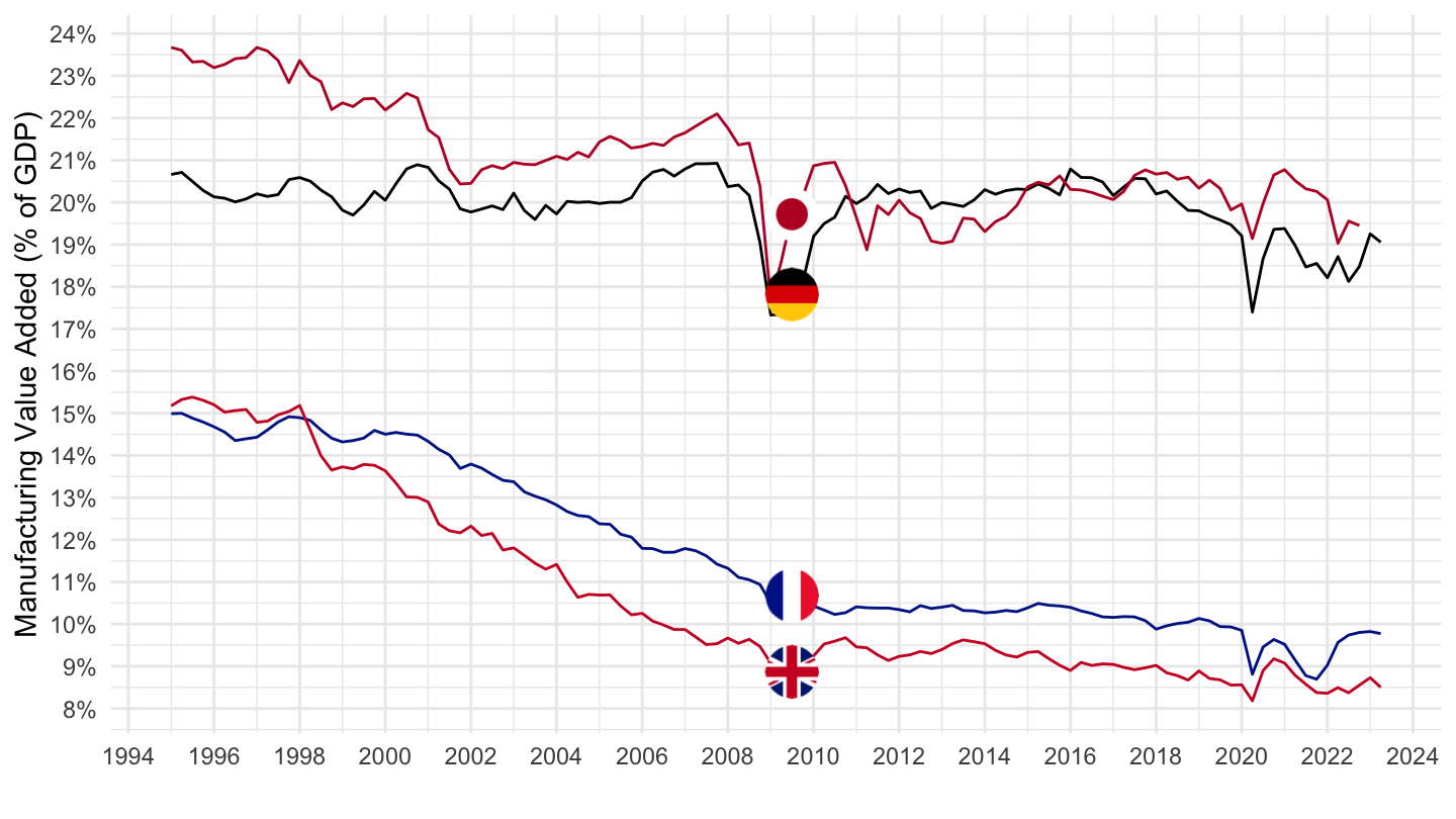
QNA |>
  filter(SUBJECT %in% c("B1GVC", "B1_GE"),
         MEASURE == "CQRSA",
         FREQUENCY == "Q",
         LOCATION %in% c("FRA", "DEU", "JPN", "CHN", "GBR")) |>
  left_join(QNA_var$LOCATION, by = "LOCATION") |>
  quarter_to_date() |>
  filter(date >= as.Date("1995-01-01")) |>
  select(LOCATION, Location, SUBJECT, date, obsValue) |>
  spread(SUBJECT, obsValue) |>
  mutate(obsValue = B1GVC / B1_GE) |>
  add_flag_color("Location") |>
  ggplot() + geom_line(aes(x = date, y = obsValue, color = color)) +
  scale_color_identity() + theme_minimal() + add_4flags +
  scale_x_date(breaks = seq(1920, 2100, 2) |> paste0("-01-01") |> as.Date(),
               labels = date_format("%Y")) +
  scale_y_continuous(breaks = 0.01*seq(-60, 60, 1),
                     labels = scales::percent_format(accuracy = 1)) +
  ylab("Manufacturing Value Added (% of GDP)") + xlab("")
QNA |>
  filter(SUBJECT %in% c("B1GVC", "B1_GE"),
         MEASURE == "CQRSA",
         FREQUENCY == "Q",
         LOCATION %in% c("ITA", "FRA", "DEU")) |>
  left_join(QNA_var$LOCATION, by = "LOCATION") |>
  quarter_to_date() |>
  select(Location, SUBJECT, date, obsValue) |>
  spread(SUBJECT, obsValue) |>
  mutate(obsValue = B1GVC / B1_GE) |>
  add_flag_color("Location") |>
  ggplot() + geom_line(aes(x = date, y = obsValue, color = color)) +
  scale_color_identity() + theme_minimal() + add_3flags +
  scale_x_date(breaks = seq(1920, 2100, 5) |> paste0("-01-01") |> as.Date(),
               labels = date_format("%Y")) +
  scale_y_continuous(breaks = 0.01*seq(-60, 60, 1),
                     labels = scales::percent_format(accuracy = 1)) +
  ylab("Manufacturing Value Added (% of GDP)") + xlab("")
QNA |>
  filter(SUBJECT %in% c("B1GVC", "B1_GE"),
         MEASURE == "CQRSA",
         FREQUENCY == "Q",
         LOCATION %in% c("CHE", "KOR", "NOR")) |>
  left_join(QNA_var$LOCATION, by = "LOCATION") |>
  quarter_to_date() |>
  select(Location, SUBJECT, date, obsValue) |>
  spread(SUBJECT, obsValue) |>
  mutate(obsValue = B1GVC / B1_GE) |>
  add_flag_color("Location") |>
  ggplot() + geom_line(aes(x = date, y = obsValue, color = color)) +
  scale_color_identity() + theme_minimal() + add_3flags +
  scale_x_date(breaks = seq(1920, 2100, 5) |> paste0("-01-01") |> as.Date(),
               labels = date_format("%Y")) +
  scale_y_continuous(breaks = 0.01*seq(-60, 60, 1),
                     labels = scales::percent_format(accuracy = 1)) +
  ylab("Manufacturing Value Added (% of GDP)") + xlab("")
QNA |>
  filter(SUBJECT %in% c("B1GVC", "B1_GE"),
         MEASURE == "CQRSA",
         FREQUENCY == "Q",
         LOCATION %in% c("FIN", "CRI", "SWE")) |>
  left_join(QNA_var$LOCATION, by = "LOCATION") |>
  quarter_to_date() |>
  select(Location, SUBJECT, date, obsValue) |>
  spread(SUBJECT, obsValue) |>
  mutate(obsValue = B1GVC / B1_GE) |>
  add_flag_color("Location") |>
  ggplot() + geom_line(aes(x = date, y = obsValue, color = color)) +
  scale_color_identity() + theme_minimal() + add_3flags +
  scale_x_date(breaks = seq(1920, 2100, 2) |> paste0("-01-01") |> as.Date(),
               labels = date_format("%Y")) +
  scale_y_continuous(breaks = 0.01*seq(-60, 60, 1),
                     labels = scales::percent_format(accuracy = 1)) +
  ylab("Manufacturing Value Added (% of GDP)") + xlab("")
QNA |>
  filter(SUBJECT %in% c("B1GVC", "B1_GE"),
         MEASURE == "LNBQRSA",
         FREQUENCY == "Q",
         LOCATION %in% c("ITA", "FRA", "DEU")) |>
  left_join(QNA_var$LOCATION, by = "LOCATION") |>
  quarter_to_date() |>
  select(Location, SUBJECT, date, obsValue) |>
  spread(SUBJECT, obsValue) |>
  mutate(obsValue = B1GVC / B1_GE) |>
  add_flag_color("Location") |>
  ggplot() + geom_line(aes(x = date, y = obsValue, color = color)) +
  scale_color_identity() + theme_minimal() + add_3flags +
  scale_x_date(breaks = seq(1920, 2100, 5) |> paste0("-01-01") |> as.Date(),
               labels = date_format("%Y")) +
  scale_y_continuous(breaks = 0.01*seq(-60, 60, 1),
                     labels = scales::percent_format(accuracy = 1)) +
  ylab("Manufacturing Value Added (% of GDP)") + xlab("")
QNA |>
  filter(SUBJECT %in% c("B1GVC", "B1_GE"),
         MEASURE == "LNBQRSA",
         FREQUENCY == "Q",
         LOCATION %in% c("FRA", "DEU")) |>
  left_join(QNA_var$LOCATION, by = "LOCATION") |>
  quarter_to_date() |>
  select(Location, SUBJECT, date, obsValue) |>
  spread(SUBJECT, obsValue) |>
  mutate(obsValue = B1GVC / B1_GE) |>
  add_flag_color("Location") |>
  ggplot() + geom_line(aes(x = date, y = obsValue, color = color)) +
  scale_color_identity() + theme_minimal() + add_2flags +
  scale_x_date(breaks = seq(1920, 2100, 5) |> paste0("-01-01") |> as.Date(),
               labels = date_format("%Y")) +
  scale_y_continuous(breaks = 0.01*seq(-60, 60, 1),
                     labels = scales::percent_format(accuracy = 1)) +
  ylab("Manufacturing Value Added (% of GDP)") + xlab("")
QNA |>
  filter(SUBJECT %in% c("B1GVC", "B1_GE"),
         MEASURE == "LNBQRSA",
         FREQUENCY == "Q",
         LOCATION %in% c("FRA", "DEU")) |>
  left_join(QNA_var$LOCATION, by = "LOCATION") |>
  quarter_to_date() |>
  filter(date >= as.Date("1995-01-01")) |>
  select(Location, SUBJECT, date, obsValue) |>
  spread(SUBJECT, obsValue) |>
  mutate(obsValue = B1GVC / B1_GE) |>
  add_flag_color("Location") |>
  ggplot() + geom_line(aes(x = date, y = obsValue, color = color)) +
  scale_color_identity() + theme_minimal() + add_2flags +
  scale_x_date(breaks = seq(1920, 2100, 2) |> paste0("-01-01") |> as.Date(),
               labels = date_format("%Y")) +
  scale_y_continuous(breaks = 0.01*seq(-60, 60, 1),
                     labels = scales::percent_format(accuracy = 1)) +
  ylab("Manufacturing Value Added (% of GDP)") + xlab("")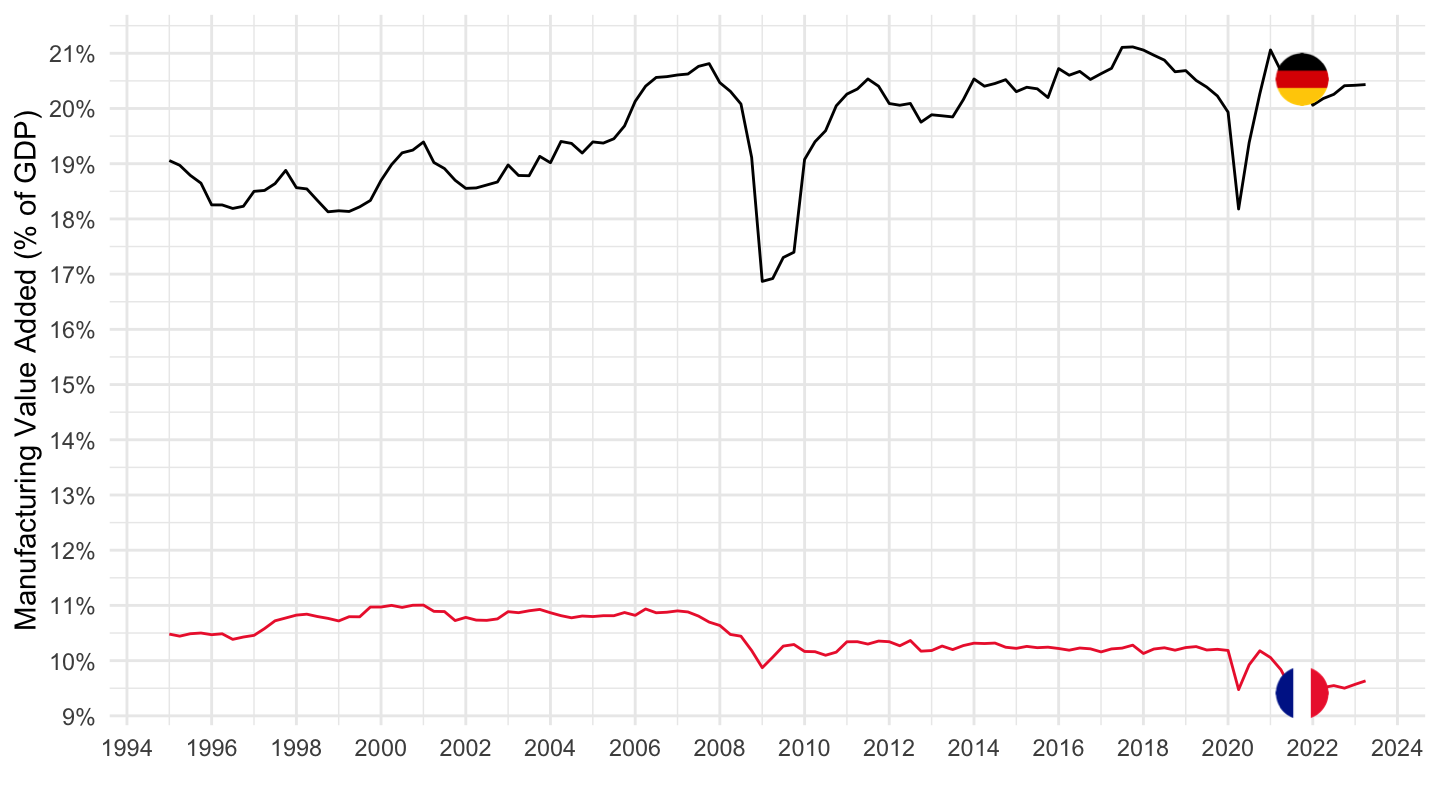
QNA |>
  filter(SUBJECT %in% c("B1GVB_E"),
         MEASURE == "CQRSA",
         FREQUENCY == "Q") |>
  left_join(QNA_var$LOCATION, by = "LOCATION") |>
  group_by(LOCATION, Location) |>
  quarter_to_date() |>
  summarise(first = first(date),
            last = last(date),
            Nobs = n()) |>
  arrange(first) |>
  mutate(Loc = gsub(" ", "-", str_to_lower(Location)),
         Loc = paste0('<img src="../../icon/flag/vsmall/', Loc, '.png" alt="Flag">')) |>
  select(Loc, everything()) %>%
{if (is_html_output()) datatable(., filter = 'top', rownames = F, escape = F) else .}QNA |>
filter(SUBJECT %in% c("B1GVB_E", "B1_GE"),
MEASURE == "CQRSA",
FREQUENCY == "Q",
LOCATION %in% c("FRA", "DEU")) |>
left_join(QNA_var$LOCATION, by = "LOCATION") |>
quarter_to_date() |>
select(Location, SUBJECT, date, obsValue) |>
spread(SUBJECT, obsValue) |>
mutate(obsValue = B1GVB_E / B1_GE) |>
add_flag_color("Location") |>
ggplot() + geom_line(aes(x = date, y = obsValue, color = color)) +
scale_color_identity() + theme_minimal() + add_2flags +
scale_x_date(breaks = seq(1920, 2100, 5) |> paste0("-01-01") |> as.Date(),
labels = date_format("%Y")) +
scale_y_continuous(breaks = 0.01*seq(-60, 60, 1),
labels = scales::percent_format(accuracy = 1)) +
ylab("Industry Value Added (% of GDP)") + xlab("")
QNA |>
  filter(SUBJECT %in% c("B1GVB_E", "B1_GE"),
         MEASURE == "CQRSA",
         FREQUENCY == "Q",
         LOCATION %in% c("FRA", "DEU")) |>
  left_join(QNA_var$LOCATION, by = "LOCATION") |>
  quarter_to_date() |>
  filter(date >= as.Date("1995-01-01")) |>
  select(Location, SUBJECT, date, obsValue) |>
  spread(SUBJECT, obsValue) |>
  mutate(obsValue = B1GVB_E / B1_GE) |>
  add_flag_color("Location") |>
  ggplot() + geom_line(aes(x = date, y = obsValue, color = color)) +
  scale_color_identity() + theme_minimal() + add_2flags +
  scale_x_date(breaks = seq(1920, 2100, 5) |> paste0("-01-01") |> as.Date(),
               labels = date_format("%Y")) +
  scale_y_continuous(breaks = 0.01*seq(-60, 60, 1),
                     labels = scales::percent_format(accuracy = 1)) +
  ylab("Industry Value Added (% of GDP)") + xlab("")
QNA |>
  filter(SUBJECT %in% c("B1GVB_E", "B1_GE"),
         MEASURE == "CQRSA",
         FREQUENCY == "Q",
         LOCATION %in% c("ITA", "FRA", "DEU")) |>
  left_join(QNA_var$LOCATION, by = "LOCATION") |>
  quarter_to_date() |>
  select(Location, SUBJECT, date, obsValue) |>
  spread(SUBJECT, obsValue) |>
  mutate(obsValue = B1GVB_E / B1_GE) |>
  add_flag_color("Location") |>
  ggplot() + geom_line(aes(x = date, y = obsValue, color = color)) +
  scale_color_identity() + theme_minimal() + add_3flags +
  scale_x_date(breaks = seq(1920, 2100, 5) |> paste0("-01-01") |> as.Date(),
               labels = date_format("%Y")) +
  scale_y_continuous(breaks = 0.01*seq(-60, 60, 1),
                     labels = scales::percent_format(accuracy = 1)) +
  ylab("Industry Value Added (% of GDP)") + xlab("")
QNA |>
  filter(SUBJECT %in% c("B1GVB_E", "B1_GE"),
         MEASURE == "CQRSA",
         FREQUENCY == "Q",
         LOCATION %in% c("ITA", "FRA", "DEU")) |>
  left_join(QNA_var$LOCATION, by = "LOCATION") |>
  quarter_to_date() |>
  filter(date >= as.Date("1995-01-01")) |>
  select(Location, SUBJECT, date, obsValue) |>
  spread(SUBJECT, obsValue) |>
  mutate(obsValue = B1GVB_E / B1_GE) |>
  add_flag_color("Location") |>
  ggplot() + geom_line(aes(x = date, y = obsValue, color = color)) +
  scale_color_identity() + theme_minimal() + add_3flags +
  scale_x_date(breaks = seq(1920, 2100, 2) |> paste0("-01-01") |> as.Date(),
               labels = date_format("%Y")) +
  scale_y_continuous(breaks = 0.01*seq(-60, 60, 1),
                     labels = scales::percent_format(accuracy = 1)) +
  ylab("Industry Value Added (% of GDP)") + xlab("")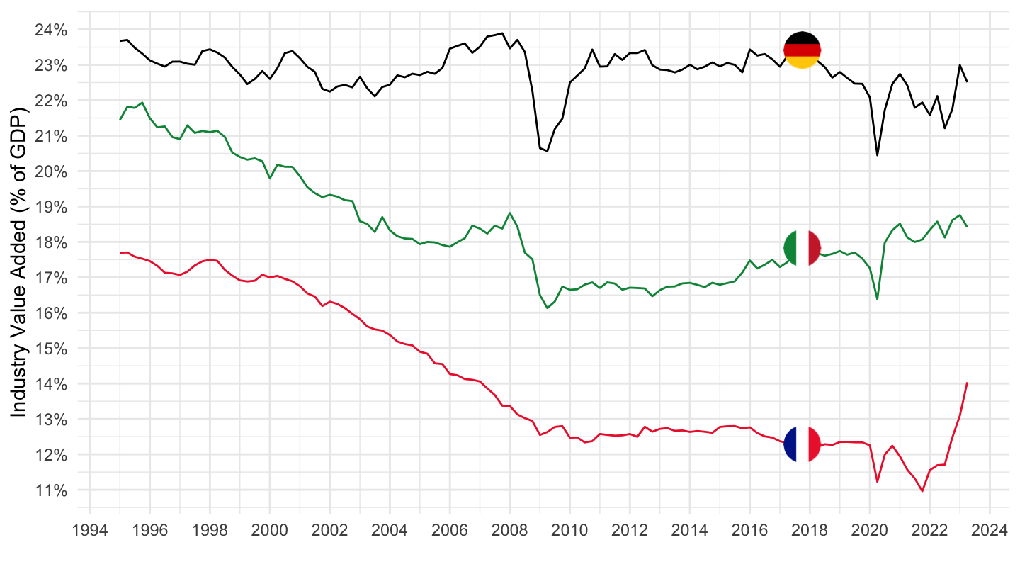
| source | dataset | Title | Updated |
|---|---|---|---|
| source | dataset | Title | Updated |
|---|---|---|---|




