Info

source	dataset	.html	.RData
oecd	QNA	2024-04-15	2024-04-15
oecd	SNA_TABLE3	2024-04-15	2024-04-11

Data on macro

source	dataset	.html	.RData
eurostat	nama_10_a10	2024-04-15	2024-04-09
eurostat	nama_10_a10_e	2024-04-15	2024-04-09
eurostat	nama_10_gdp	2024-04-15	2024-04-09
eurostat	nama_10_lp_ulc	2024-04-15	2024-04-15
eurostat	namq_10_a10	2024-04-15	2024-04-15
eurostat	namq_10_a10_e	2024-04-15	2024-04-15
eurostat	namq_10_gdp	2024-04-15	2024-04-09
eurostat	namq_10_lp_ulc	2024-04-15	2024-04-09
eurostat	namq_10_pc	2024-04-15	2024-04-09
eurostat	nasa_10_nf_tr	2024-04-15	2024-04-09
eurostat	nasq_10_nf_tr	2024-04-15	2024-04-15
fred	gdp	2024-04-15	2024-04-15
oecd	QNA	2024-04-15	2024-04-15
oecd	SNA_TABLE1	2024-04-15	2024-04-15
oecd	SNA_TABLE14A	2024-04-15	2024-04-15
oecd	SNA_TABLE2	2024-04-15	2024-04-11
oecd	SNA_TABLE6A	2024-04-15	2024-04-15
wdi	NE.RSB.GNFS.ZS	2024-04-14	2024-04-14
wdi	NY.GDP.MKTP.CD	2024-04-14	2024-04-14
wdi	NY.GDP.MKTP.PP.CD	2024-04-14	2024-04-14
wdi	NY.GDP.PCAP.CD	2024-04-14	2024-04-14
wdi	NY.GDP.PCAP.KD	2024-04-14	2024-04-14
wdi	NY.GDP.PCAP.PP.CD	2024-04-14	2024-04-14
wdi	NY.GDP.PCAP.PP.KD	2024-04-14	2024-04-14

Last

obsTime	Nobs
2023-Q4	1916

Real GDP Last

QNA Live

QNA %>%
  filter(FREQUENCY == "Q",
         SUBJECT == "B1_GE",
         MEASURE == "VOBARSA") %>%
  quarter_to_date %>%
  filter(date >= as.Date("2019-10-01")) %>%
  group_by(LOCATION) %>%
  arrange(date) %>%
  mutate(obsValue = 100*obsValue/obsValue[date == as.Date("2019-10-01")],
         obsValue = cumsum(obsValue) / seq_along(obsValue)) %>%
  group_by(LOCATION) %>%
  do(tail(., 1)) %>%
  left_join(LOCATION, by = "LOCATION") %>%
  select(LOCATION, Location, date, obsValue) %>%
  arrange(obsValue) %>%
  mutate(Flag = gsub(" ", "-", str_to_lower(Location)),
         Flag = paste0('<img src="../../icon/flag/vsmall/', Flag, '.png" alt="Flag">')) %>%
  select(Flag, everything()) %>%
  {if (is_html_output()) datatable(., filter = 'top', rownames = F, escape = F) else .}

Last, France

QNA %>%
  filter(LOCATION == "FRA",
         FREQUENCY == "Q") %>%
  left_join(QNA_var$SUBJECT, by = "SUBJECT") %>%
  left_join(QNA_var$MEASURE, by = "MEASURE") %>%
  select(SUBJECT, Subject, MEASURE, Measure, obsTime, obsValue) %>%
  arrange(SUBJECT, MEASURE) %>%
  group_by(SUBJECT, Subject, MEASURE, Measure) %>%
  summarise(first_t = first(obsTime),
            last_t = last(obsTime),
            first_v = first(obsValue),
            last_v = last(obsValue)) %>%
  {if (is_html_output()) datatable(., filter = 'top', rownames = F, escape = F) else .}

Last, Germany

QNA %>%
  filter(LOCATION == "DEU",
         FREQUENCY == "Q") %>%
  left_join(QNA_var$SUBJECT, by = "SUBJECT") %>%
  left_join(QNA_var$MEASURE, by = "MEASURE") %>%
  select(SUBJECT, Subject, MEASURE, Measure, obsTime, obsValue) %>%
  arrange(SUBJECT, MEASURE) %>%
  group_by(SUBJECT, Subject, MEASURE, Measure) %>%
  summarise(first_t = first(obsTime),
            last_t = last(obsTime),
            first_v = first(obsValue),
            last_v = last(obsValue)) %>%
  {if (is_html_output()) datatable(., filter = 'top', rownames = F, escape = F) else .}

Horse Races

Greece

Germany, US VS France

2007-

QNA %>%
  filter(LOCATION %in% c("USA", "DEU", "GRC", "FRA"),
         SUBJECT == "B1_GE",
         MEASURE == "VOBARSA",
         FREQUENCY == "Q") %>%
  quarter_to_date %>%
  left_join(QNA_var$LOCATION, by = "LOCATION") %>%
  mutate(Location = ifelse(LOCATION == "EA20", "Europe", Location)) %>%
  select(LOCATION, Location, date, B1_GE_VOBARSA = obsValue) %>%
  left_join(SNA_TABLE3 %>%
              filter(TRANSACT == "POPNC",
                     MEASURE == "PER") %>%
              year_to_date %>%
              select(LOCATION, date, POPNC_PER = obsValue), 
            by = c("date", "LOCATION")) %>%
  filter(date >= as.Date("1999-10-01"),
         month(date) %% 3 == 1) %>%
  mutate(date = date + months(3) -days(1)) %>%
  select(LOCATION, Location, date, B1_GE_VOBARSA, POPNC_PER) %>%
  group_by(LOCATION, Location) %>%
  mutate(POPNC_PER_i = spline(x = date, y = POPNC_PER, xout = date)$y,
         obsValue = B1_GE_VOBARSA/POPNC_PER_i) %>%
  arrange(date) %>%
  mutate(obsValue = 100 * obsValue / obsValue[date == as.Date("2007-06-30")]) %>%
  left_join(colors, by = c("Location" = "country")) %>%
  ggplot(.) + theme_minimal() + xlab("") + ylab("PIB par habitant (2007 = 100)") +
  geom_line(aes(x = date, y = obsValue, color = color)) + add_4flags +
  scale_color_identity() +
  scale_x_date(breaks = seq(1960, 2030, 2) %>% paste0("-01-01") %>% as.Date,
               labels = date_format("%Y")) +
  theme(legend.position = "none") +
  scale_y_log10(breaks = seq(50, 200, 5))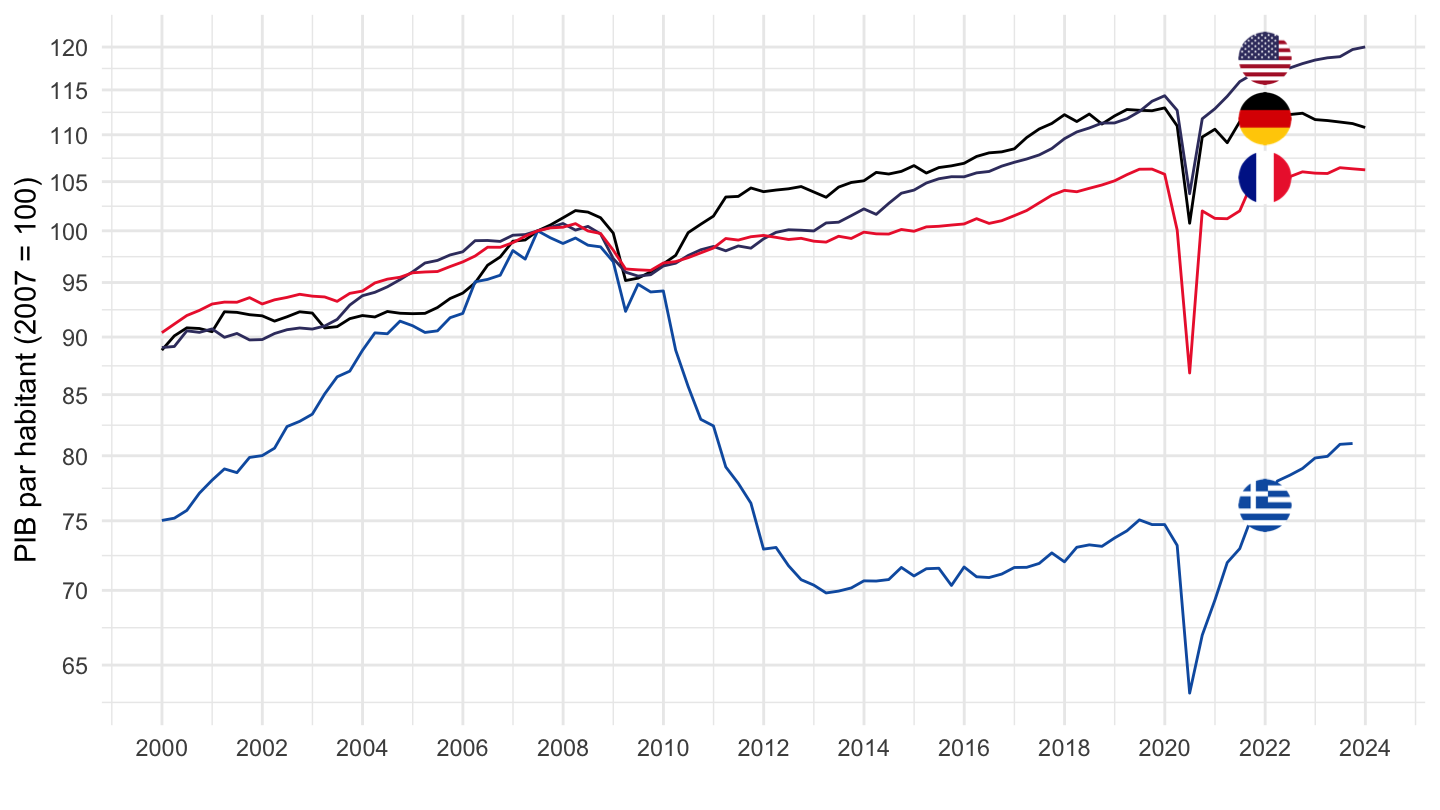

2001- (introduction Euro)

QNA %>%
  filter(LOCATION %in% c("USA", "DEU", "GRC", "FRA"),
         SUBJECT == "B1_GE",
         MEASURE == "VOBARSA",
         FREQUENCY == "Q") %>%
  quarter_to_date %>%
  left_join(QNA_var$LOCATION, by = "LOCATION") %>%
  mutate(Location = ifelse(LOCATION == "EA20", "Europe", Location)) %>%
  select(LOCATION, Location, date, B1_GE_VOBARSA = obsValue) %>%
  left_join(SNA_TABLE3 %>%
              filter(TRANSACT == "POPNC",
                     MEASURE == "PER") %>%
              year_to_date %>%
              select(LOCATION, date, POPNC_PER = obsValue), 
            by = c("date", "LOCATION")) %>%
  filter(date >= as.Date("2000-10-01"),
         month(date) %% 3 == 1) %>%
  mutate(date = date + months(3) -days(1)) %>%
  select(LOCATION, Location, date, B1_GE_VOBARSA, POPNC_PER) %>%
  group_by(LOCATION, Location) %>%
  mutate(POPNC_PER_i = spline(x = date, y = POPNC_PER, xout = date)$y,
         obsValue = B1_GE_VOBARSA/POPNC_PER_i) %>%
  arrange(date) %>%
  mutate(obsValue = 100 * obsValue / obsValue[date == as.Date("2000-12-31")]) %>%
  left_join(colors, by = c("Location" = "country")) %>%
  ggplot(.) + theme_minimal() + xlab("") + ylab("GDP Per Capita (2001 = 100)") +
  geom_line(aes(x = date, y = obsValue, color = color)) + add_4flags +
  scale_color_identity() +
  scale_x_date(breaks = seq(1961, 2030, 2) %>% paste0("-01-01") %>% as.Date,
               labels = date_format("%Y")) +
  theme(legend.position = "none") +
  scale_y_log10(breaks = seq(50, 200, 5)) + 
  geom_hline(yintercept = 100, linetype = "dashed")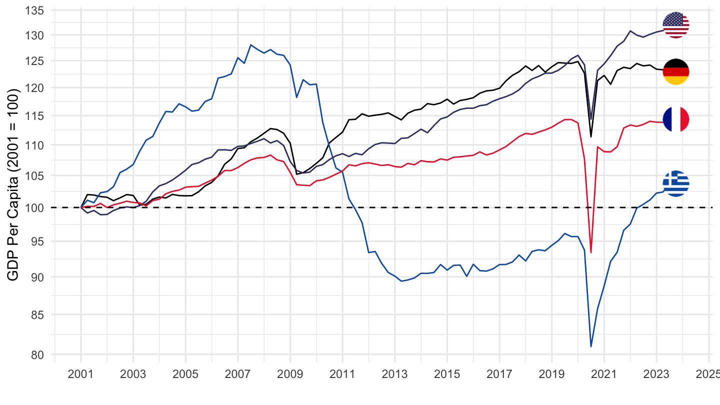

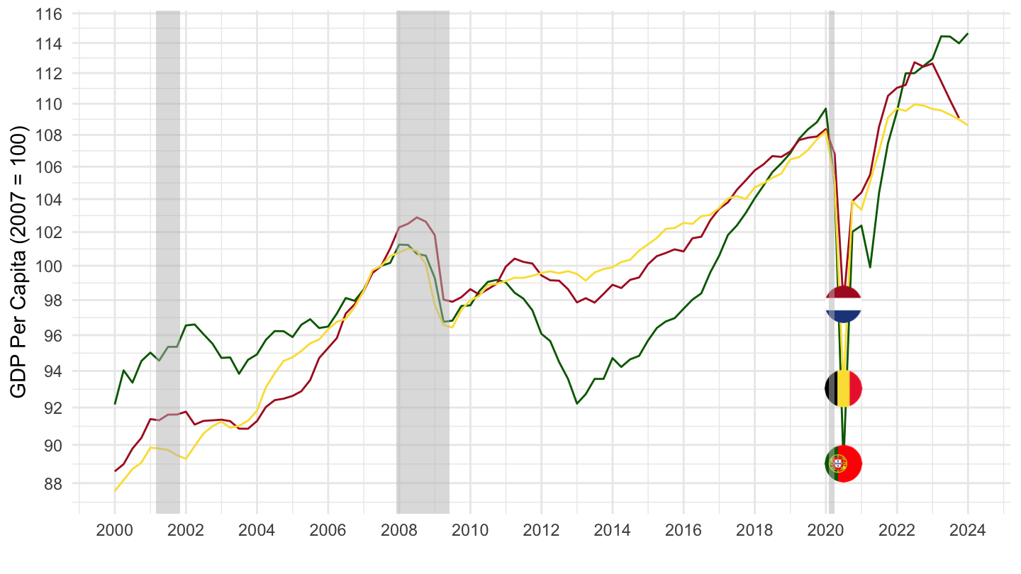
With Italy

Base 2007

QNA %>%
  filter(LOCATION %in% c("USA", "DEU", "GRC", "FRA", "ITA"),
         SUBJECT == "B1_GE",
         MEASURE == "VOBARSA",
         FREQUENCY == "Q") %>%
  quarter_to_date %>%
  left_join(QNA_var$LOCATION, by = "LOCATION") %>%
  mutate(Location = ifelse(LOCATION == "EA20", "Europe", Location)) %>%
  select(LOCATION, Location, date, B1_GE_VOBARSA = obsValue) %>%
  left_join(SNA_TABLE3 %>%
              filter(TRANSACT == "POPNC",
                     MEASURE == "PER") %>%
              year_to_date %>%
              select(LOCATION, date, POPNC_PER = obsValue), 
            by = c("date", "LOCATION")) %>%
  filter(date >= as.Date("1999-10-01"),
         month(date) %% 3 == 1) %>%
  mutate(date = date + months(3) -days(1)) %>%
  select(LOCATION, Location, date, B1_GE_VOBARSA, POPNC_PER) %>%
  group_by(LOCATION, Location) %>%
  mutate(POPNC_PER_i = spline(x = date, y = POPNC_PER, xout = date)$y,
         obsValue = B1_GE_VOBARSA/POPNC_PER_i) %>%
  arrange(date) %>%
  mutate(obsValue = 100 * obsValue / obsValue[date == as.Date("2007-06-30")]) %>%
  left_join(colors, by = c("Location" = "country")) %>%
  ggplot(.) + theme_minimal() + xlab("") + ylab("GDP Per Capita (2007 = 100)") +
  geom_line(aes(x = date, y = obsValue, color = color)) + add_5flags +
  scale_color_identity() +
  scale_x_date(breaks = seq(1960, 2030, 2) %>% paste0("-01-01") %>% as.Date,
               labels = date_format("%Y")) +
  theme(legend.position = "none") +
  scale_y_log10(breaks = seq(50, 200, 5))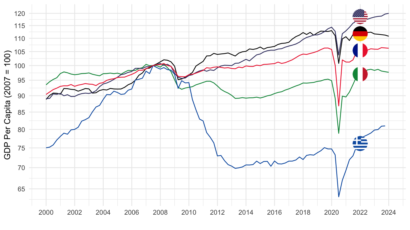

Base 2001

QNA %>%
  filter(LOCATION %in% c("USA", "DEU", "GRC", "FRA", "ITA"),
         SUBJECT == "B1_GE",
         MEASURE == "VOBARSA",
         FREQUENCY == "Q") %>%
  quarter_to_date %>%
  left_join(QNA_var$LOCATION, by = "LOCATION") %>%
  mutate(Location = ifelse(LOCATION == "EA20", "Europe", Location)) %>%
  select(LOCATION, Location, date, B1_GE_VOBARSA = obsValue) %>%
  left_join(SNA_TABLE3 %>%
              filter(TRANSACT == "POPNC",
                     MEASURE == "PER") %>%
              year_to_date %>%
              select(LOCATION, date, POPNC_PER = obsValue), 
            by = c("date", "LOCATION")) %>%
  filter(date >= as.Date("2000-10-01"),
         month(date) %% 3 == 1) %>%
  mutate(date = date + months(3) -days(1)) %>%
  select(LOCATION, Location, date, B1_GE_VOBARSA, POPNC_PER) %>%
  group_by(LOCATION, Location) %>%
  mutate(POPNC_PER_i = spline(x = date, y = POPNC_PER, xout = date)$y,
         obsValue = B1_GE_VOBARSA/POPNC_PER_i) %>%
  arrange(date) %>%
  mutate(obsValue = 100 * obsValue / obsValue[date == as.Date("2000-12-31")]) %>%
  left_join(colors, by = c("Location" = "country")) %>%
  ggplot(.) + theme_minimal() + xlab("") + ylab("GDP Per Capita (2001 = 100)") +
  geom_line(aes(x = date, y = obsValue, color = color)) + add_5flags +
  scale_color_identity() +
  scale_x_date(breaks = seq(1960, 2030, 2) %>% paste0("-01-01") %>% as.Date,
               labels = date_format("%Y")) +
  theme(legend.position = "none") +
  scale_y_log10(breaks = seq(50, 200, 5))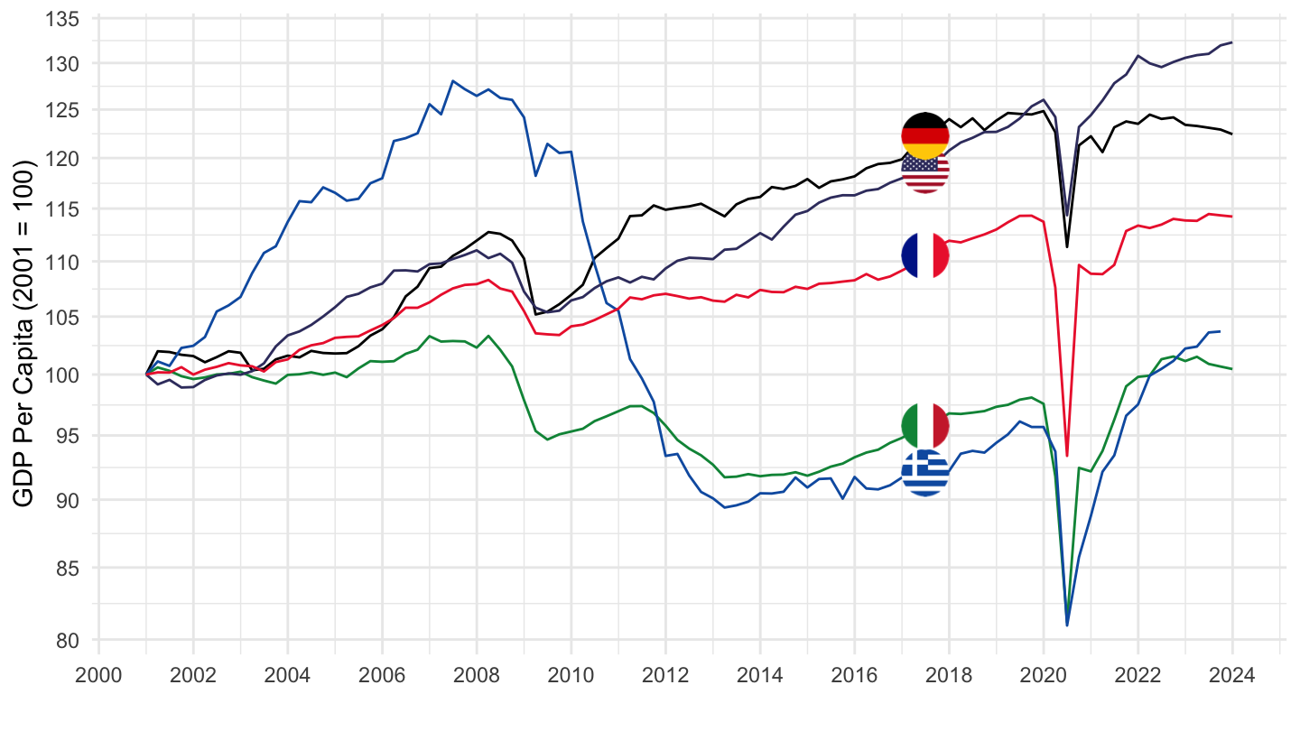

French

QNA %>%
  filter(LOCATION %in% c("GRC", "FRA", "ISL"),
         SUBJECT == "B1_GE",
         MEASURE == "VOBARSA",
         FREQUENCY == "Q") %>%
  quarter_to_date %>%
  left_join(QNA_var$LOCATION, by = "LOCATION") %>%
  mutate(Location = ifelse(LOCATION == "EA20", "Europe", Location)) %>%
  select(LOCATION, Location, date, B1_GE_VOBARSA = obsValue) %>%
  left_join(SNA_TABLE3 %>%
              filter(TRANSACT == "POPNC",
                     MEASURE == "PER") %>%
              year_to_date %>%
              select(LOCATION, date, POPNC_PER = obsValue), 
            by = c("date", "LOCATION")) %>%
  filter(date >= as.Date("1999-10-01"),
         month(date) %% 3 == 1) %>%
  mutate(date = date + months(3) -days(1)) %>%
  select(LOCATION, Location, date, B1_GE_VOBARSA, POPNC_PER) %>%
  group_by(LOCATION, Location) %>%
  mutate(POPNC_PER_i = spline(x = date, y = POPNC_PER, xout = date)$y,
         obsValue = B1_GE_VOBARSA/POPNC_PER_i) %>%
  arrange(date) %>%
  mutate(obsValue = 100 * obsValue / obsValue[date == as.Date("2007-06-30")]) %>%
  left_join(colors, by = c("Location" = "country")) %>%
  ggplot(.) + theme_minimal() + xlab("") + ylab("PIB par habitant (100 = 2007)") +
  geom_line(aes(x = date, y = obsValue, color = color)) + add_3flags +
  scale_color_identity() +
  scale_x_date(breaks = seq(1960, 2030, 2) %>% paste0("-01-01") %>% as.Date,
               labels = date_format("%Y")) +
  theme(legend.position = "none") +
  scale_y_log10(breaks = seq(50, 200, 5))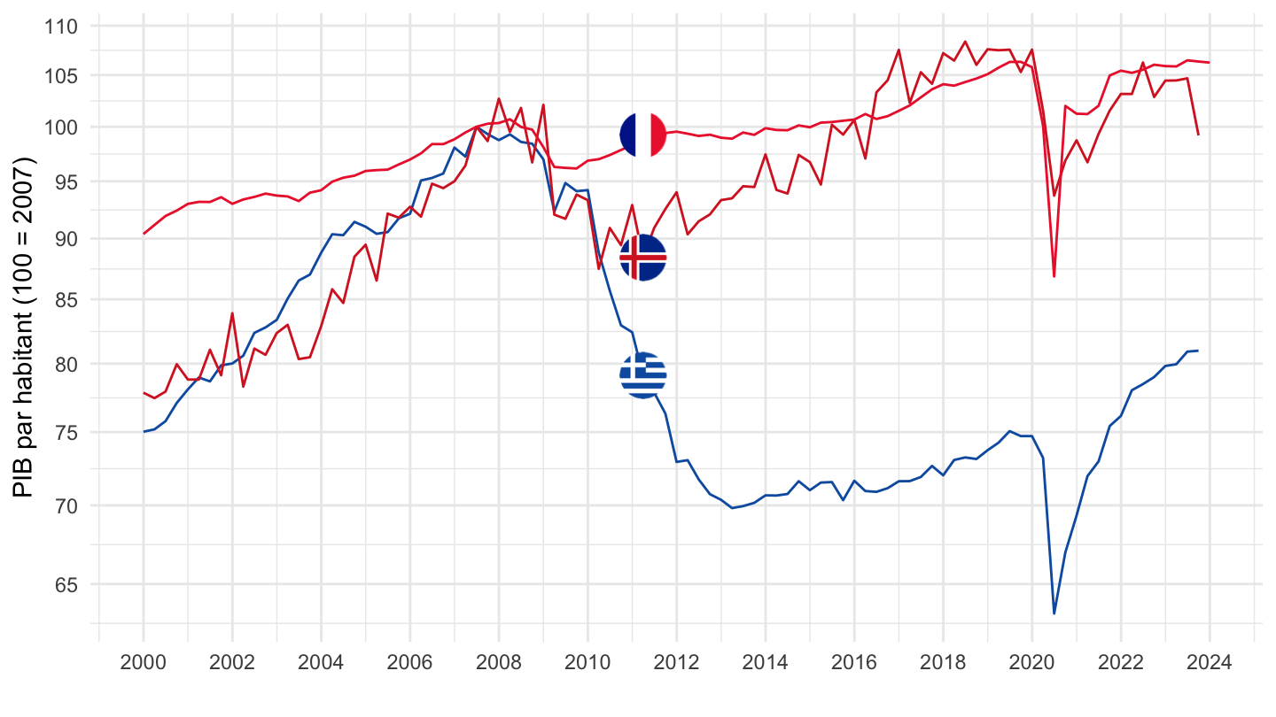

Eurozone VS Eurone

2000-

English

QNA %>%
  filter(LOCATION %in% c("EU27_2020", "EA20"),
         SUBJECT == "B1_GE",
         MEASURE == "VOBARSA",
         FREQUENCY == "Q") %>%
  quarter_to_date %>%
  left_join(QNA_var$LOCATION, by = "LOCATION") %>%
  select(LOCATION, Location, date, B1_GE_VOBARSA = obsValue) %>%
  left_join(SNA_TABLE3 %>%
              filter(TRANSACT == "POPNC",
                     MEASURE == "PER") %>%
              year_to_date %>%
              select(LOCATION, date, POPNC_PER = obsValue), 
            by = c("date", "LOCATION")) %>%
  filter(date >= as.Date("1999-10-01"),
         month(date) %% 3 == 1) %>%
  mutate(date = date + months(3) -days(1)) %>%
  mutate(Location2 = Location) %>%
  mutate(Location = ifelse(LOCATION == "EA20", "Europe", Location),
         Location = ifelse(LOCATION == "EU27_2020", "Europe", Location)) %>%
  select(Location2, Location, LOCATION, date, B1_GE_VOBARSA, POPNC_PER) %>%
  group_by(LOCATION) %>%
  mutate(POPNC_PER_i = spline(x = date, y = POPNC_PER, xout = date)$y,
         obsValue = B1_GE_VOBARSA/POPNC_PER_i) %>%
  arrange(date) %>%
  mutate(obsValue = 100 * obsValue / obsValue[date == as.Date("2007-06-30")]) %>%
  ggplot(.) + theme_minimal() + xlab("") + ylab("Real GDP Per Capita (2007 = 100)") +
  geom_line(aes(x = date, y = obsValue, color = Location2)) + add_2flags +
  geom_rect(data = nber_recessions %>%
              filter(Peak >= as.Date("1995-01-01")), 
            aes(xmin = Peak, xmax = Trough, ymin = 0, ymax = +Inf), 
            fill = 'grey', alpha = 0.5) +
  scale_color_manual(values = c("#003399", "#FFCC00")) +
  scale_x_date(breaks = seq(1960,2100,  2) %>% paste0("-01-01") %>% as.Date,
               labels = date_format("%Y")) +
  theme(legend.position = c(0.35, 0.9),
        legend.title = element_blank()) +
  #theme(legend.position = "none") +
  scale_y_log10(breaks = seq(70, 200, 2))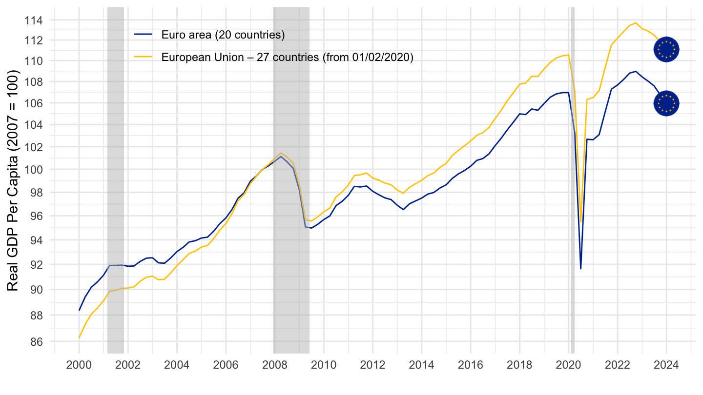

US VS Europe

2000-

population

QNA %>%
  filter(LOCATION %in% c("USA", "EA20"),
         SUBJECT %in% c("B1_GE"),
         MEASURE == "VOBARSA",
         FREQUENCY == "Q") %>%
  quarter_to_date %>%
  left_join(QNA_var$LOCATION, by = "LOCATION") %>%
  select(SUBJECT, LOCATION, Location, date, obsValue) %>%
  left_join(SNA_TABLE3 %>%
              filter(TRANSACT == "POPNC",
                     MEASURE == "PER") %>%
              year_to_date %>%
              select(LOCATION, date, POPNC_PER = obsValue), 
            by = c("date", "LOCATION")) %>%
  filter(date >= as.Date("1999-10-01"),
         month(date) %% 3 == 1) %>%
  mutate(date = date + months(3) -days(1)) %>%
  mutate(Location = ifelse(LOCATION == "EA20", "Euro area", "US")) %>%
  select(SUBJECT,Location, LOCATION, date, obsValue, POPNC_PER) %>%
  group_by(SUBJECT, LOCATION) %>%
  mutate(POPNC_PER_i = spline(x = date, y = POPNC_PER, xout = date)$y) %>%
  ungroup %>%
  select(LOCATION, date, POPNC_PER, POPNC_PER_i) %>%
  gather(variable, value, -date, -LOCATION) %>%
  ggplot(.) + theme_minimal() + xlab("") + ylab("2008Q1 = 100") +
  geom_line(aes(x = date, y = value, color = variable, linetype = LOCATION))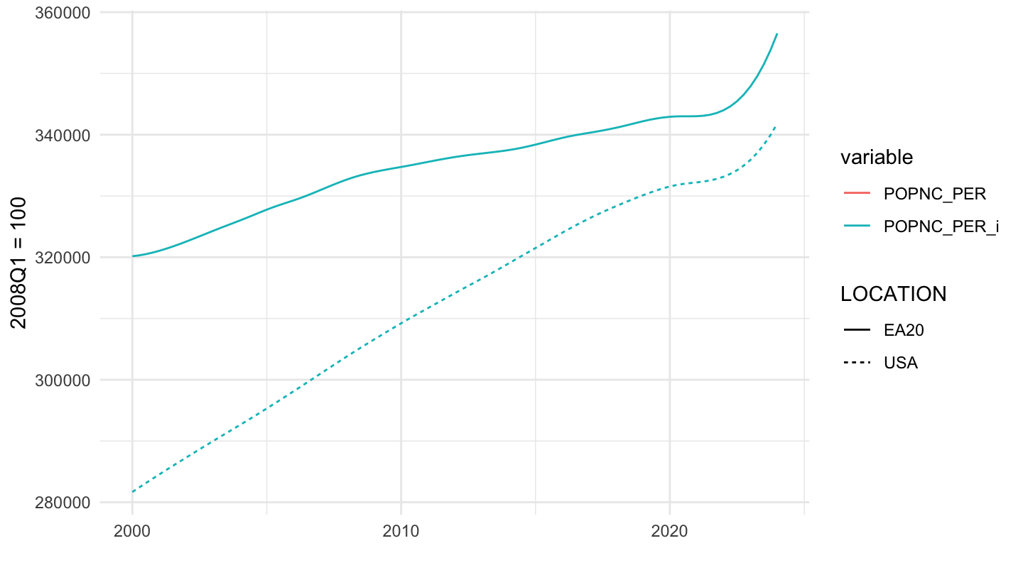

English

QNA %>%
  filter(LOCATION %in% c("USA", "EA20"),
         SUBJECT %in% c("B1_GE", "P31S14_S15", "P51"),
         MEASURE == "VOBARSA",
         FREQUENCY == "Q") %>%
  quarter_to_date %>%
  left_join(QNA_var$LOCATION, by = "LOCATION") %>%
  select(SUBJECT, LOCATION, Location, date, obsValue) %>%
  left_join(SNA_TABLE3 %>%
              filter(TRANSACT == "POPNC",
                     MEASURE == "PER") %>%
              year_to_date %>%
              select(LOCATION, date, POPNC_PER = obsValue), 
            by = c("date", "LOCATION")) %>%
  filter(date >= as.Date("1999-10-01"),
         month(date) %% 3 == 1) %>%
  mutate(date = date + months(3) -days(1)) %>%
  mutate(Location = ifelse(LOCATION == "EA20", "Euro area", "US")) %>%
  select(SUBJECT,Location, LOCATION, date, obsValue, POPNC_PER) %>%
  group_by(SUBJECT, LOCATION) %>%
  mutate(POPNC_PER_i = spline(x = date, y = POPNC_PER, xout = date)$y) %>%
  mutate(obsValue = obsValue/POPNC_PER_i) %>%
  arrange(date) %>%
  mutate(obsValue = 100 * obsValue / obsValue[date == as.Date("2007-12-31")]) %>%
  ungroup %>%
  mutate(Subject = case_when(SUBJECT == "B1_GE" ~ "GDP / capita",
                             SUBJECT == "P31S14_S15" ~ "Consumption / capita",
                             SUBJECT == "P51" ~ "Investment / capita")) %>%
  mutate(Subject = factor(Subject, levels = c("GDP / capita", "Consumption / capita", "Investment / capita"))) %>%
  ggplot(.) + theme_minimal() + xlab("") + ylab("2008Q1 = 100") +
  geom_line(aes(x = date, y = obsValue, color = Location)) + add_2flags +
  geom_rect(data = nber_recessions %>%
              filter(Peak >= as.Date("1995-01-01")), 
            aes(xmin = Peak, xmax = Trough, ymin = 0, ymax = +Inf), 
            fill = 'grey', alpha = 0.5) +
  scale_color_manual(values = c("#003399", "#BF0A30")) +
  scale_x_date(breaks = seq(1960,2100,  5) %>% paste0("-01-01") %>% as.Date,
               labels = date_format("%Y")) +
  theme(legend.position = "top",
        legend.title = element_blank(),
        axis.text.x = element_text(angle = 45, vjust = 1, hjust = 1)) +
  scale_y_log10(breaks = seq(70, 200, 2)) +
  facet_wrap(~ Subject)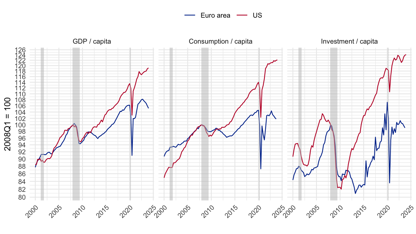

French

QNA %>%
  filter(LOCATION %in% c("USA", "EA20"),
         SUBJECT %in% c("B1_GE", "P31S14_S15", "P51"),
         MEASURE == "VOBARSA",
         FREQUENCY == "Q") %>%
  quarter_to_date %>%
  left_join(QNA_var$LOCATION, by = "LOCATION") %>%
  select(SUBJECT, LOCATION, Location, date, obsValue) %>%
  left_join(SNA_TABLE3 %>%
              filter(TRANSACT == "POPNC",
                     MEASURE == "PER") %>%
              year_to_date %>%
              select(LOCATION, date, POPNC_PER = obsValue), 
            by = c("date", "LOCATION")) %>%
  filter(date >= as.Date("1999-10-01"),
         month(date) %% 3 == 1) %>%
  mutate(date = date + months(3) -days(1)) %>%
  mutate(Location = ifelse(LOCATION == "EA20", "Zone euro", "États-Unis"),
         Location = factor(Location, levels = c("Zone euro", "États-Unis"))) %>%
  select(SUBJECT,Location, LOCATION, date, obsValue, POPNC_PER) %>%
  group_by(SUBJECT, LOCATION) %>%
  mutate(POPNC_PER_i = spline(x = date, y = POPNC_PER, xout = date)$y,
         obsValue = obsValue/POPNC_PER_i) %>%
  arrange(date) %>%
  mutate(obsValue = 100 * obsValue / obsValue[date == as.Date("2007-12-31")]) %>%
  ungroup %>%
  mutate(Subject = case_when(SUBJECT == "B1_GE" ~ "PIB / habitant",
                             SUBJECT == "P31S14_S15" ~ "Consommation / habitant",
                             SUBJECT == "P51" ~ "Investissement / habitant")) %>%
  mutate(Subject = factor(Subject, levels = c("PIB / habitant", "Consommation / habitant", "Investissement / habitant"))) %>%
  ggplot(.) + theme_minimal() + xlab("") + ylab("1er trimestre 2008 = 100") +
  geom_line(aes(x = date, y = obsValue, color = Location)) + add_2flags +
  geom_rect(data = nber_recessions %>%
              filter(Peak >= as.Date("1995-01-01")), 
            aes(xmin = Peak, xmax = Trough, ymin = 0, ymax = +Inf), 
            fill = 'grey', alpha = 0.5) +
  scale_color_manual(values = c("#003399", "#BF0A30")) +
  scale_x_date(breaks = seq(1960,2100,  5) %>% paste0("-01-01") %>% as.Date,
               labels = date_format("%Y")) +
  theme(legend.position = "top",
        legend.title = element_blank(),
        axis.text.x = element_text(angle = 45, vjust = 1, hjust = 1)) +
  scale_y_log10(breaks = seq(70, 200, 2)) +
  facet_wrap(~ Subject)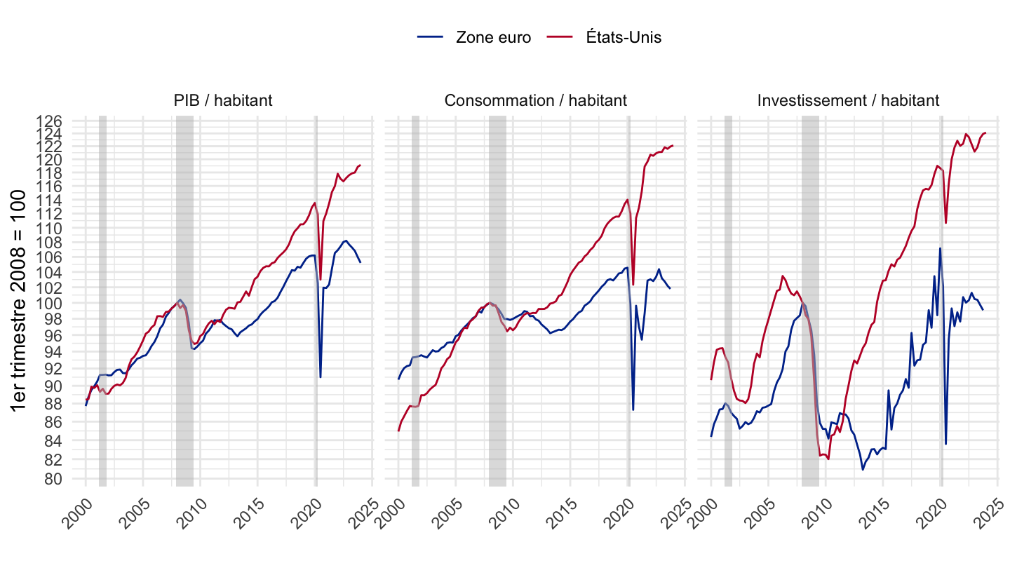

Flags

QNA %>%
  filter(LOCATION %in% c("USA", "EA20"),
         SUBJECT %in% c("B1_GE", "P31S14_S15", "P51"),
         MEASURE == "VOBARSA",
         FREQUENCY == "Q") %>%
  quarter_to_date %>%
  left_join(QNA_var$LOCATION, by = "LOCATION") %>%
  select(SUBJECT, LOCATION, Location, date, obsValue) %>%
  left_join(SNA_TABLE3 %>%
              filter(TRANSACT == "POPNC",
                     MEASURE == "PER") %>%
              year_to_date %>%
              select(LOCATION, date, POPNC_PER = obsValue), 
            by = c("date", "LOCATION")) %>%
  filter(date >= as.Date("1999-10-01"),
         month(date) %% 3 == 1) %>%
  mutate(date = date + months(3) -days(1)) %>%
  mutate(Location2 = ifelse(LOCATION == "EA20", "Zone euro", "États-Unis"),
         Location2 = factor(Location2, levels = c("Zone euro", "États-Unis"))) %>%
  mutate(Location = ifelse(LOCATION == "EA20", "Europe", "United States")) %>%
  select(SUBJECT,Location, Location2, LOCATION, date, obsValue, POPNC_PER) %>%
  group_by(SUBJECT, LOCATION) %>%
  mutate(POPNC_PER_i = spline(x = date, y = POPNC_PER, xout = date)$y,
         obsValue = obsValue/POPNC_PER_i) %>%
  arrange(date) %>%
  mutate(obsValue = 100 * obsValue / obsValue[date == as.Date("2007-12-31")]) %>%
  ungroup %>%
  mutate(Subject = case_when(SUBJECT == "B1_GE" ~ "PIB / habitant",
                             SUBJECT == "P31S14_S15" ~ "Consommation / habitant",
                             SUBJECT == "P51" ~ "Investissement / habitant")) %>%
  mutate(Subject = factor(Subject, levels = c("PIB / habitant", "Consommation / habitant", "Investissement / habitant"))) %>%
  ggplot(.) + theme_minimal() + xlab("") + ylab("1er trimestre 2008 = 100") +
  geom_line(aes(x = date, y = obsValue, color = Location2)) +
  geom_image(data = . %>%
               filter(date == as.Date("2015-12-31")) %>%
               mutate(image = paste0("../../icon/flag/round/", str_to_lower(gsub(" ", "-", Location)), ".png")),
             aes(x = date, y = obsValue, image = image), asp = 1.5) +
  geom_rect(data = nber_recessions %>%
              filter(Peak >= as.Date("1995-01-01")), 
            aes(xmin = Peak, xmax = Trough, ymin = 0, ymax = +Inf), 
            fill = 'grey', alpha = 0.5) +
  scale_color_manual(values = c("#003399", "#BF0A30")) +
  scale_x_date(breaks = seq(1960,2100,  5) %>% paste0("-01-01") %>% as.Date,
               labels = date_format("%Y")) +
  theme(legend.position = "top",
        legend.title = element_blank(),
        axis.text.x = element_text(angle = 45, vjust = 1, hjust = 1)) +
  scale_y_log10(breaks = seq(70, 200, 2)) +
  facet_wrap(~ Subject)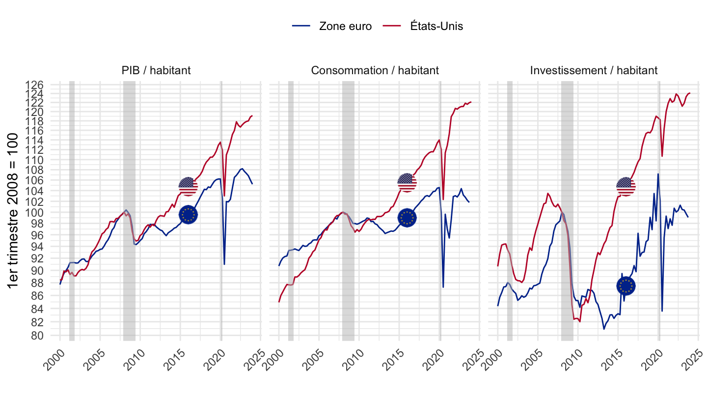

French

QNA %>%
  filter(LOCATION %in% c("USA", "EA20"),
         SUBJECT %in% c("B1_GE", "P31S14_S15"),
         MEASURE == "VOBARSA",
         FREQUENCY == "Q") %>%
  quarter_to_date %>%
  left_join(QNA_var$LOCATION, by = "LOCATION") %>%
  select(SUBJECT, LOCATION, Location, date, obsValue) %>%
  left_join(SNA_TABLE3 %>%
              filter(TRANSACT == "POPNC",
                     MEASURE == "PER") %>%
              year_to_date %>%
              select(LOCATION, date, POPNC_PER = obsValue), 
            by = c("date", "LOCATION")) %>%
  filter(date >= as.Date("1999-10-01"),
         month(date) %% 3 == 1) %>%
  mutate(date = date + months(3) -days(1)) %>%
  mutate(Location2 = ifelse(LOCATION == "EA20", "Zone euro", "États-Unis"),
         Location2 = factor(Location2, levels = c("Zone euro", "États-Unis"))) %>%
  mutate(Location = ifelse(LOCATION == "EA20", "Europe", "United States")) %>%
  select(SUBJECT,Location, Location2, LOCATION, date, obsValue, POPNC_PER) %>%
  group_by(SUBJECT, LOCATION) %>%
  mutate(POPNC_PER_i = spline(x = date, y = POPNC_PER, xout = date)$y,
         obsValue = obsValue/POPNC_PER_i) %>%
  arrange(date) %>%
  mutate(obsValue = 100 * obsValue / obsValue[date == as.Date("2007-12-31")]) %>%
  ungroup %>%
  mutate(Subject = case_when(SUBJECT == "B1_GE" ~ "PIB / habitant",
                             SUBJECT == "P31S14_S15" ~ "Consommation / habitant",
                             SUBJECT == "P51" ~ "Investissement / habitant")) %>%
  mutate(Subject = factor(Subject, levels = c("PIB / habitant", "Consommation / habitant", "Investissement / habitant"))) %>%
  ggplot(.) + theme_minimal() + xlab("") + ylab("1er trimestre 2008 = 100") +
  geom_line(aes(x = date, y = obsValue, color = Location2)) + add_2flags +
  geom_rect(data = nber_recessions %>%
              filter(Peak >= as.Date("1995-01-01")), 
            aes(xmin = Peak, xmax = Trough, ymin = 0, ymax = +Inf), 
            fill = 'grey', alpha = 0.5) +
  scale_color_manual(values = c("#003399", "#BF0A30")) + add_4flags +
  scale_x_date(breaks = seq(1960,2100,  5) %>% paste0("-01-01") %>% as.Date,
               labels = date_format("%Y")) +
  theme(legend.position = "top",
        legend.title = element_blank(),
        axis.text.x = element_text(angle = 45, vjust = 1, hjust = 1)) +
  scale_y_log10(breaks = seq(70, 200, 2)) +
  facet_wrap(~ Subject)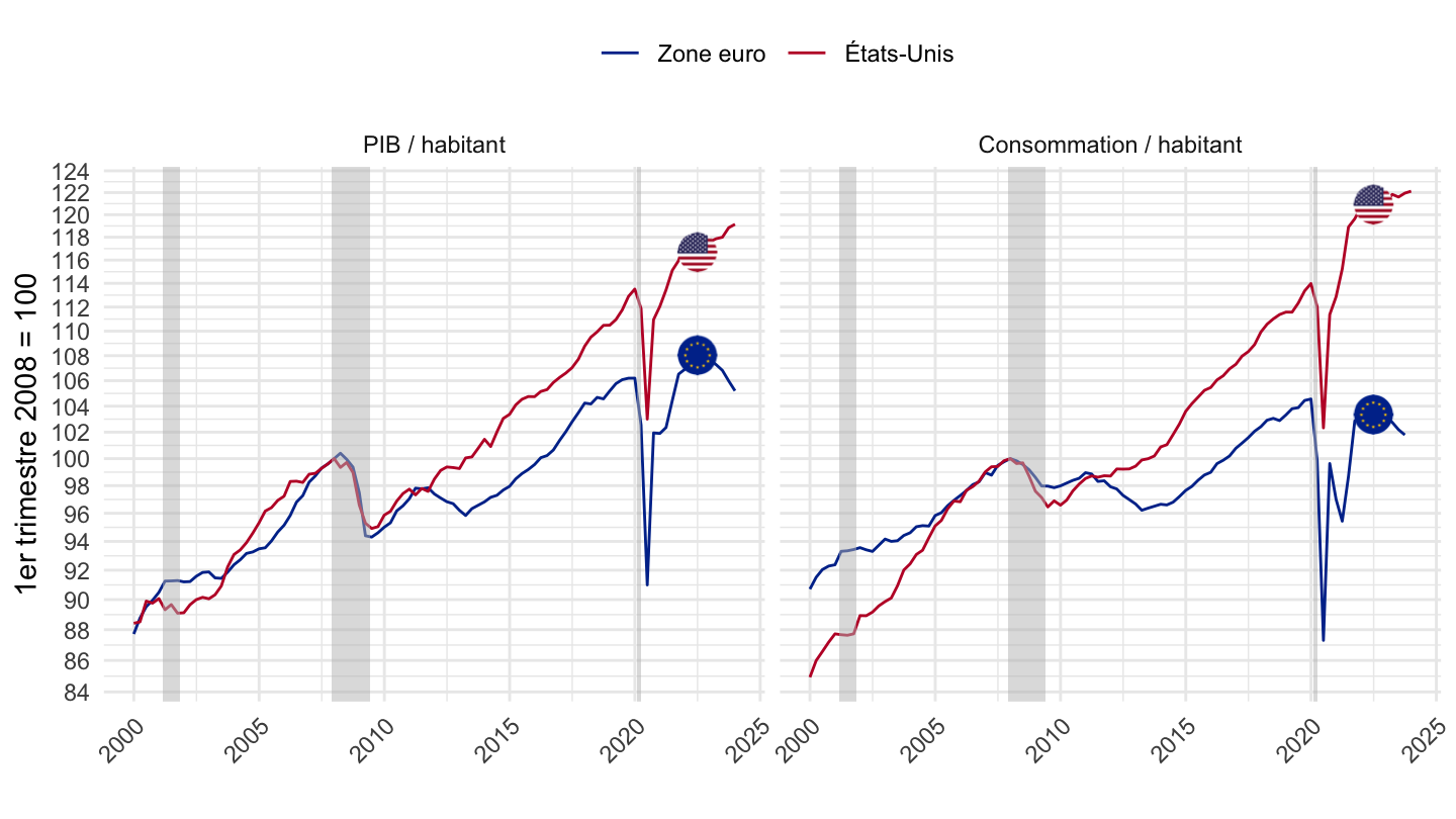

US VS Europe

2000-

English

QNA %>%
  filter(LOCATION %in% c("USA", "EA20"),
         SUBJECT == "B1_GE",
         MEASURE == "VOBARSA",
         FREQUENCY == "Q") %>%
  quarter_to_date %>%
  left_join(QNA_var$LOCATION, by = "LOCATION") %>%
  select(LOCATION, Location, date, B1_GE_VOBARSA = obsValue) %>%
  left_join(SNA_TABLE3 %>%
              filter(TRANSACT == "POPNC",
                     MEASURE == "PER") %>%
              year_to_date %>%
              select(LOCATION, date, POPNC_PER = obsValue), 
            by = c("date", "LOCATION")) %>%
  filter(date >= as.Date("1999-10-01"),
         month(date) %% 3 == 1) %>%
  mutate(date = date + months(3) -days(1)) %>%
  mutate(Location = ifelse(LOCATION == "EA20", "Europe", Location)) %>%
  select(Location, LOCATION, date, B1_GE_VOBARSA, POPNC_PER) %>%
  group_by(LOCATION) %>%
  mutate(POPNC_PER_i = spline(x = date, y = POPNC_PER, xout = date)$y,
         obsValue = B1_GE_VOBARSA/POPNC_PER_i) %>%
  arrange(date) %>%
  mutate(obsValue = 100 * obsValue / obsValue[date == as.Date("2007-06-30")]) %>%
  ggplot(.) + theme_minimal() + xlab("") + ylab("Real GDP Per Capita (2007 = 100)") +
  geom_line(aes(x = date, y = obsValue, color = Location)) + add_2flags +
  geom_rect(data = nber_recessions %>%
              filter(Peak >= as.Date("1995-01-01")), 
            aes(xmin = Peak, xmax = Trough, ymin = 0, ymax = +Inf), 
            fill = 'grey', alpha = 0.5) +
  scale_color_manual(values = c("#003399", "#BF0A30")) +
  scale_x_date(breaks = seq(1960,2100,  2) %>% paste0("-01-01") %>% as.Date,
               labels = date_format("%Y")) +
  theme(legend.position = "none") +
  scale_y_log10(breaks = seq(70, 200, 2))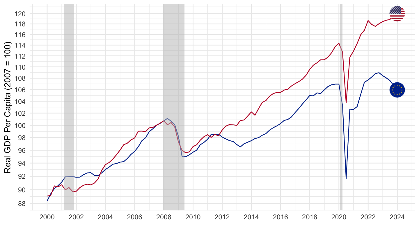

French (Base = 2007)

All

QNA %>%
  filter(LOCATION %in% c("USA", "EA20"),
         SUBJECT == "B1_GE",
         MEASURE == "VOBARSA",
         FREQUENCY == "Q") %>%
  quarter_to_date %>%
  left_join(QNA_var$LOCATION, by = "LOCATION") %>%
  select(LOCATION, Location, date, B1_GE_VOBARSA = obsValue) %>%
  left_join(SNA_TABLE3 %>%
              filter(TRANSACT == "POPNC",
                     MEASURE == "PER") %>%
              year_to_date %>%
              select(LOCATION, date, POPNC_PER = obsValue), 
            by = c("date", "LOCATION")) %>%
  filter(date >= as.Date("1999-10-01"),
         month(date) %% 3 == 1) %>%
  mutate(date = date + months(3) -days(1)) %>%
  mutate(Location = ifelse(LOCATION == "EA20", "Europe", Location)) %>%
  select(Location, LOCATION, date, B1_GE_VOBARSA, POPNC_PER) %>%
  group_by(LOCATION) %>%
  mutate(POPNC_PER_i = spline(x = date, y = POPNC_PER, xout = date)$y,
         obsValue = B1_GE_VOBARSA/POPNC_PER_i) %>%
  arrange(date) %>%
  mutate(obsValue = 100 * obsValue / obsValue[date == as.Date("2007-06-30")]) %>%
  ggplot(.) + theme_minimal() + xlab("") + ylab("PIB par habitant (2007 = 100)") +
  geom_line(aes(x = date, y = obsValue, color = Location)) + add_2flags +
  geom_rect(data = nber_recessions %>%
              filter(Peak >= as.Date("1995-01-01")), 
            aes(xmin = Peak, xmax = Trough, ymin = 0, ymax = +Inf), 
            fill = 'grey', alpha = 0.5) +
  scale_color_manual(values = c("#003399", "#BF0A30")) +
  scale_x_date(breaks = seq(1960,2100,  2) %>% paste0("-01-01") %>% as.Date,
               labels = date_format("%Y")) +
  theme(legend.position = "none") +
  scale_y_log10(breaks = seq(70, 200, 2))

With ticks

GDP per capita

QNA %>%
  filter(LOCATION %in% c("USA", "EA20"),
         SUBJECT == "B1_GE",
         MEASURE == "VOBARSA",
         FREQUENCY == "Q") %>%
  quarter_to_date %>%
  left_join(QNA_var$LOCATION, by = "LOCATION") %>%
  select(LOCATION, Location, date, B1_GE_VOBARSA = obsValue) %>%
  left_join(SNA_TABLE3 %>%
              filter(TRANSACT == "POPNC",
                     MEASURE == "PER") %>%
              year_to_date %>%
              select(LOCATION, date, POPNC_PER = obsValue), 
            by = c("date", "LOCATION")) %>%
  filter(date >= as.Date("1999-10-01"),
         month(date) %% 3 == 1) %>%
  mutate(date = date + months(3) -days(1)) %>%
  mutate(Location = ifelse(LOCATION == "EA20", "Europe", Location)) %>%
  select(Location, LOCATION, date, B1_GE_VOBARSA, POPNC_PER) %>%
  group_by(LOCATION) %>%
  mutate(POPNC_PER_i = spline(x = date, y = POPNC_PER, xout = date)$y,
         obsValue = B1_GE_VOBARSA/POPNC_PER_i) %>%
  arrange(date) %>%
  mutate(obsValue = 100 * obsValue / obsValue[date == as.Date("2007-06-30")]) %>%
  select(date, obsValue, Location) %>%
  ggplot(.) + theme_minimal() + xlab("") + ylab("PIB par habitant (2007 = 100)") +
  geom_line(aes(x = date, y = obsValue, color = Location)) + add_2flags +
  geom_rect(data = nber_recessions %>%
              filter(Peak >= as.Date("1995-01-01")), 
            aes(xmin = Peak, xmax = Trough, ymin = 0, ymax = +Inf), 
            fill = 'grey', alpha = 0.5) +
  scale_color_manual(values = c("#003399", "#BF0A30")) +
  scale_x_date(breaks = seq(1960,2100,  2) %>% paste0("-01-01") %>% as.Date,
               labels = date_format("%Y")) +
  theme(legend.position = "none") +
  scale_y_log10(breaks = seq(70, 200, 2)) +
  geom_text_repel(aes(x = date, y = obsValue, label = round(obsValue, 1)), 
                  fontface ="plain", color = "black", size = 3,
                  max.overlaps = 10)

Consumption per capita

QNA %>%
  filter(LOCATION %in% c("USA", "EA20"),
         SUBJECT == "P31S14_S15",
         MEASURE == "VOBARSA",
         FREQUENCY == "Q") %>%
  quarter_to_date %>%
  left_join(QNA_var$LOCATION, by = "LOCATION") %>%
  select(LOCATION, Location, date, B1_GE_VOBARSA = obsValue) %>%
  left_join(SNA_TABLE3 %>%
              filter(TRANSACT == "POPNC",
                     MEASURE == "PER") %>%
              year_to_date %>%
              select(LOCATION, date, POPNC_PER = obsValue), 
            by = c("date", "LOCATION")) %>%
  filter(date >= as.Date("1999-10-01"),
         month(date) %% 3 == 1) %>%
  mutate(date = date + months(3) -days(1)) %>%
  mutate(Location = ifelse(LOCATION == "EA20", "Europe", Location)) %>%
  select(Location, LOCATION, date, B1_GE_VOBARSA, POPNC_PER) %>%
  group_by(LOCATION) %>%
  mutate(POPNC_PER_i = spline(x = date, y = POPNC_PER, xout = date)$y,
         obsValue = B1_GE_VOBARSA/POPNC_PER_i) %>%
  arrange(date) %>%
  mutate(obsValue = 100 * obsValue / obsValue[date == as.Date("2007-06-30")]) %>%
  select(date, obsValue, Location) %>%
  ggplot(.) + theme_minimal() + xlab("") + ylab("Consommation par habitant (2007 = 100)") +
  geom_line(aes(x = date, y = obsValue, color = Location)) + add_2flags +
  geom_rect(data = nber_recessions %>%
              filter(Peak >= as.Date("1995-01-01")), 
            aes(xmin = Peak, xmax = Trough, ymin = 0, ymax = +Inf), 
            fill = 'grey', alpha = 0.5) +
  scale_color_manual(values = c("#003399", "#BF0A30")) +
  scale_x_date(breaks = seq(1960,2100,  2) %>% paste0("-01-01") %>% as.Date,
               labels = date_format("%Y")) +
  theme(legend.position = "none") +
  scale_y_log10(breaks = seq(70, 200, 2)) +
  geom_text_repel(aes(x = date, y = obsValue, label = round(obsValue, 1)), 
                  fontface ="plain", color = "black", size = 3,
                  max.overlaps = 12)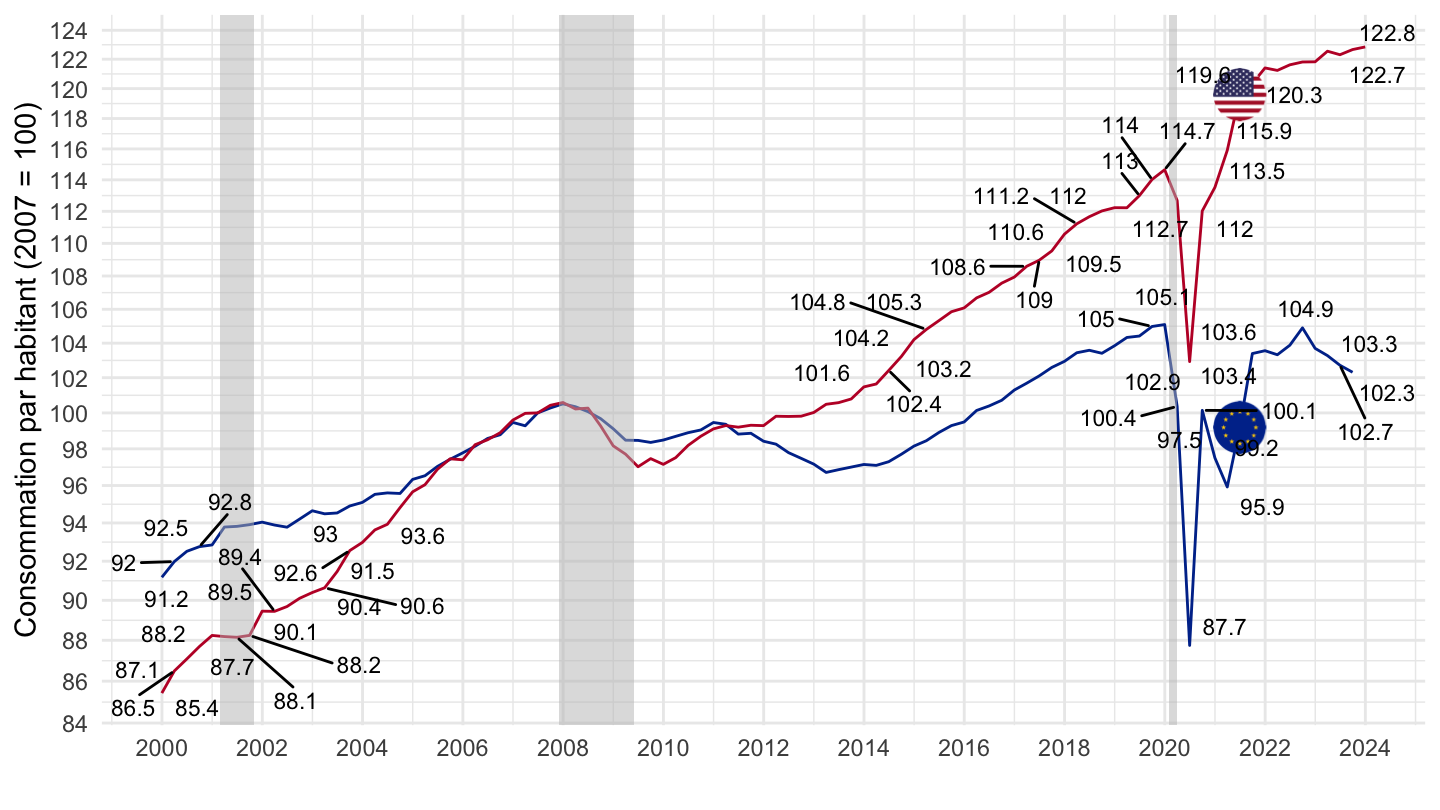

Investment per capita

QNA %>%
  filter(LOCATION %in% c("USA", "EA20"),
         SUBJECT == "P51",
         MEASURE == "VOBARSA",
         FREQUENCY == "Q") %>%
  quarter_to_date %>%
  left_join(QNA_var$LOCATION, by = "LOCATION") %>%
  select(LOCATION, Location, date, B1_GE_VOBARSA = obsValue) %>%
  left_join(SNA_TABLE3 %>%
              filter(TRANSACT == "POPNC",
                     MEASURE == "PER") %>%
              year_to_date %>%
              select(LOCATION, date, POPNC_PER = obsValue), 
            by = c("date", "LOCATION")) %>%
  filter(date >= as.Date("1999-10-01"),
         month(date) %% 3 == 1) %>%
  mutate(date = date + months(3) -days(1)) %>%
  mutate(Location = ifelse(LOCATION == "EA20", "Europe", Location)) %>%
  select(Location, LOCATION, date, B1_GE_VOBARSA, POPNC_PER) %>%
  group_by(LOCATION) %>%
  mutate(POPNC_PER_i = spline(x = date, y = POPNC_PER, xout = date)$y,
         obsValue = B1_GE_VOBARSA/POPNC_PER_i) %>%
  arrange(date) %>%
  mutate(obsValue = 100 * obsValue / obsValue[date == as.Date("2007-06-30")]) %>%
  select(date, obsValue, Location) %>%
  ggplot(.) + theme_minimal() + xlab("") + ylab("Investissement par habitant (2007 = 100)") +
  geom_line(aes(x = date, y = obsValue, color = Location)) + add_2flags +
  geom_rect(data = nber_recessions %>%
              filter(Peak >= as.Date("1995-01-01")), 
            aes(xmin = Peak, xmax = Trough, ymin = 0, ymax = +Inf), 
            fill = 'grey', alpha = 0.5) +
  scale_color_manual(values = c("#003399", "#BF0A30")) +
  scale_x_date(breaks = seq(1960,2100,  2) %>% paste0("-01-01") %>% as.Date,
               labels = date_format("%Y")) +
  theme(legend.position = "none") +
  scale_y_log10(breaks = seq(70, 200, 2)) +
  geom_text_repel(aes(x = date, y = obsValue, label = round(obsValue, 1)), 
                  fontface ="plain", color = "black", size = 3,
                  max.overlaps = 10)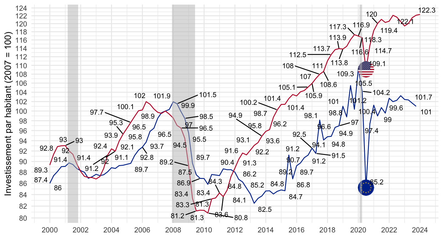

French (Base = 2014)

QNA %>%
  filter(LOCATION %in% c("USA", "EA20"),
         SUBJECT == "B1_GE",
         MEASURE == "VOBARSA",
         FREQUENCY == "Q") %>%
  quarter_to_date %>%
  left_join(QNA_var$LOCATION, by = "LOCATION") %>%
  select(LOCATION, Location, date, B1_GE_VOBARSA = obsValue) %>%
  left_join(SNA_TABLE3 %>%
              filter(TRANSACT == "POPNC",
                     MEASURE == "PER") %>%
              year_to_date %>%
              select(LOCATION, date, POPNC_PER = obsValue), 
            by = c("date", "LOCATION")) %>%
  filter(date >= as.Date("1999-10-01"),
         month(date) %% 3 == 1) %>%
  mutate(date = date + months(3) -days(1)) %>%
  mutate(Location = ifelse(LOCATION == "EA20", "Europe", Location)) %>%
  select(Location, LOCATION, date, B1_GE_VOBARSA, POPNC_PER) %>%
  group_by(LOCATION) %>%
  mutate(POPNC_PER_i = spline(x = date, y = POPNC_PER, xout = date)$y,
         obsValue = B1_GE_VOBARSA/POPNC_PER_i) %>%
  arrange(date) %>%
  mutate(obsValue = 100 * obsValue / obsValue[date == as.Date("2014-06-30")]) %>%
  ggplot(.) + theme_minimal() + xlab("") + ylab("PIB par habitant (2014 = 100)") +
  geom_line(aes(x = date, y = obsValue, color = Location)) + add_2flags +
  geom_rect(data = nber_recessions %>%
              filter(Peak >= as.Date("1995-01-01")), 
            aes(xmin = Peak, xmax = Trough, ymin = 0, ymax = +Inf), 
            fill = 'grey', alpha = 0.5) +
  scale_color_manual(values = c("#003399", "#BF0A30")) +
  scale_x_date(breaks = seq(1960,2100,  2) %>% paste0("-01-01") %>% as.Date,
               labels = date_format("%Y")) +
  theme(legend.position = "none") +
  scale_y_log10(breaks = seq(70, 200, 2))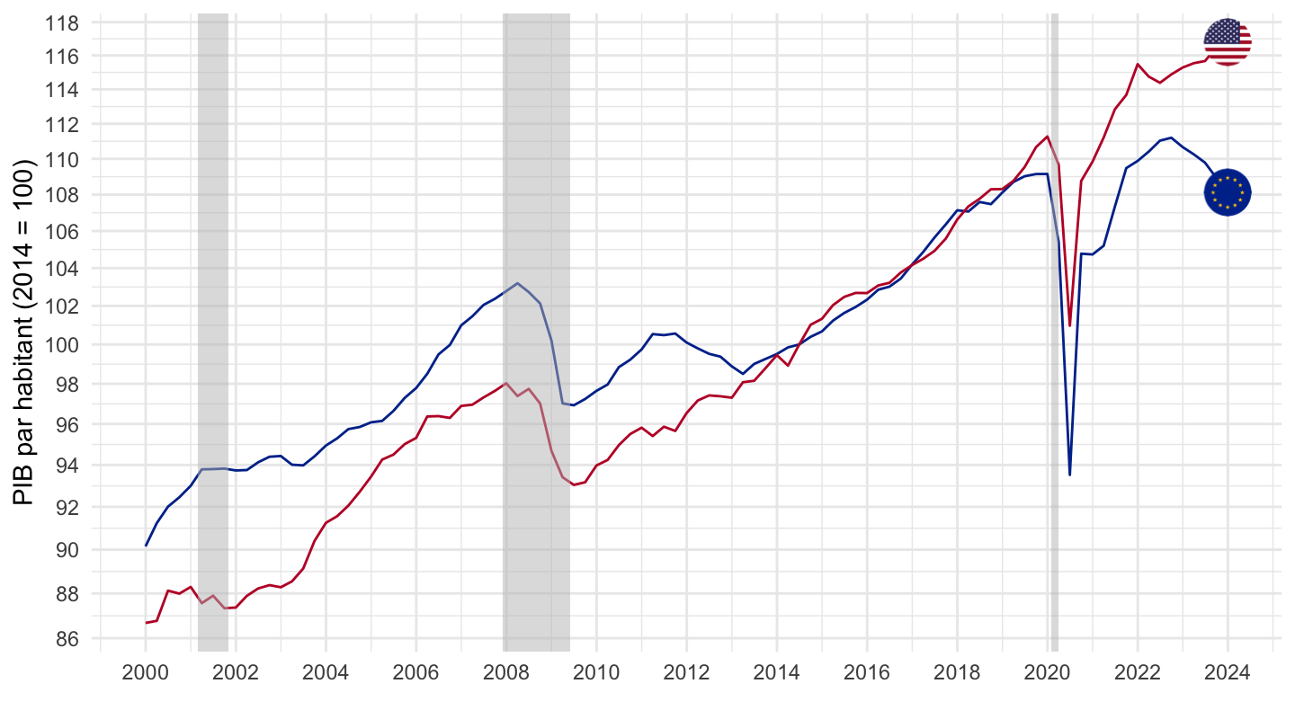

2010-

French (Base = 2007)

QNA %>%
  filter(LOCATION %in% c("USA", "EA20"),
         SUBJECT == "B1_GE",
         MEASURE == "VOBARSA",
         FREQUENCY == "Q") %>%
  quarter_to_date %>%
  left_join(QNA_var$LOCATION, by = "LOCATION") %>%
  select(LOCATION, Location, date, B1_GE_VOBARSA = obsValue) %>%
  left_join(SNA_TABLE3 %>%
              filter(TRANSACT == "POPNC",
                     MEASURE == "PER") %>%
              year_to_date %>%
              select(LOCATION, date, POPNC_PER = obsValue), 
            by = c("date", "LOCATION")) %>%
  filter(date >= as.Date("2010-01-01"),
         month(date) %% 3 == 1) %>%
  mutate(date = date + months(3) -days(1)) %>%
  mutate(Location = ifelse(LOCATION == "EA20", "Europe", Location)) %>%
  select(Location, LOCATION, date, B1_GE_VOBARSA, POPNC_PER) %>%
  group_by(LOCATION) %>%
  mutate(POPNC_PER_i = spline(x = date, y = POPNC_PER, xout = date)$y,
         obsValue = B1_GE_VOBARSA/POPNC_PER_i) %>%
  arrange(date) %>%
  mutate(obsValue = 100 * obsValue / obsValue[date == as.Date("2010-03-31")]) %>%
  ggplot(.) + theme_minimal() + xlab("") + ylab("PIB par habitant (2010 = 100)") +
  geom_line(aes(x = date, y = obsValue, color = Location)) + add_2flags +
  geom_rect(data = nber_recessions %>%
              filter(Peak >= as.Date("2010-01-01")), 
            aes(xmin = Peak, xmax = Trough, ymin = 0, ymax = +Inf), 
            fill = 'grey', alpha = 0.5) +
  scale_color_manual(values = c("#003399", "#BF0A30")) +
  scale_x_date(breaks = seq(1960,2100,  2) %>% paste0("-01-01") %>% as.Date,
               labels = date_format("%Y")) +
  theme(legend.position = "none") +
  scale_y_log10(breaks = seq(70, 200, 2))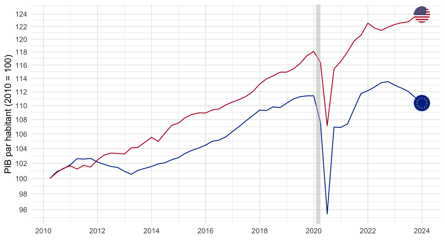

French (Base = 2014)

QNA %>%
  filter(LOCATION %in% c("USA", "EA20"),
         SUBJECT == "B1_GE",
         MEASURE == "VOBARSA",
         FREQUENCY == "Q") %>%
  quarter_to_date %>%
  left_join(QNA_var$LOCATION, by = "LOCATION") %>%
  select(LOCATION, Location, date, B1_GE_VOBARSA = obsValue) %>%
  left_join(SNA_TABLE3 %>%
              filter(TRANSACT == "POPNC",
                     MEASURE == "PER") %>%
              year_to_date %>%
              select(LOCATION, date, POPNC_PER = obsValue), 
            by = c("date", "LOCATION")) %>%
  filter(date >= as.Date("1999-10-01"),
         month(date) %% 3 == 1) %>%
  mutate(date = date + months(3) -days(1)) %>%
  mutate(Location = ifelse(LOCATION == "EA20", "Europe", Location)) %>%
  select(Location, LOCATION, date, B1_GE_VOBARSA, POPNC_PER) %>%
  group_by(LOCATION) %>%
  mutate(POPNC_PER_i = spline(x = date, y = POPNC_PER, xout = date)$y,
         obsValue = B1_GE_VOBARSA/POPNC_PER_i) %>%
  arrange(date) %>%
  mutate(obsValue = 100 * obsValue / obsValue[date == as.Date("2014-06-30")]) %>%
  ggplot(.) + theme_minimal() + xlab("") + ylab("PIB par habitant (2014 = 100)") +
  geom_line(aes(x = date, y = obsValue, color = Location)) + add_2flags +
  geom_rect(data = nber_recessions %>%
              filter(Peak >= as.Date("1995-01-01")), 
            aes(xmin = Peak, xmax = Trough, ymin = 0, ymax = +Inf), 
            fill = 'grey', alpha = 0.5) +
  scale_color_manual(values = c("#003399", "#BF0A30")) +
  scale_x_date(breaks = seq(1960,2100,  2) %>% paste0("-01-01") %>% as.Date,
               labels = date_format("%Y")) +
  theme(legend.position = "none") +
  scale_y_log10(breaks = seq(70, 200, 2))

1995-

French

QNA %>%
  filter(LOCATION %in% c("USA", "EA20"),
         SUBJECT == "B1_GE",
         MEASURE == "VOBARSA",
         FREQUENCY == "Q") %>%
  quarter_to_date %>%
  left_join(QNA_var$LOCATION, by = "LOCATION") %>%
  select(LOCATION, Location, date, B1_GE_VOBARSA = obsValue) %>%
  left_join(SNA_TABLE3 %>%
              filter(TRANSACT == "POPNC",
                     MEASURE == "PER") %>%
              year_to_date %>%
              select(LOCATION, date, POPNC_PER = obsValue), 
            by = c("date", "LOCATION")) %>%
  filter(date >= as.Date("1995-01-01"),
         month(date) %% 3 == 1) %>%
  mutate(Location = ifelse(LOCATION == "EA20", "Europe", Location)) %>%
  select(Location, LOCATION, date, B1_GE_VOBARSA, POPNC_PER) %>%
  group_by(LOCATION) %>%
  mutate(POPNC_PER_i = spline(x = date, y = POPNC_PER, xout = date)$y,
         obsValue = B1_GE_VOBARSA/POPNC_PER_i) %>%
  arrange(date) %>%
  mutate(obsValue = 100 * obsValue / obsValue[date == as.Date("1995-01-01")]) %>%
  ggplot(.) + theme_minimal() + xlab("") + ylab("PIB par habitant (1995 = 100)") +
  geom_line(aes(x = date, y = obsValue, color = Location)) + add_2flags +
  geom_rect(data = nber_recessions %>%
              filter(Peak >= as.Date("1995-01-01")), 
            aes(xmin = Peak, xmax = Trough, ymin = 0, ymax = +Inf), 
            fill = 'grey', alpha = 0.5) +
  scale_color_manual(values = c("#003399", "#BF0A30")) +
  scale_x_date(breaks = seq(1960, 2025, 5) %>% paste0("-01-01") %>% as.Date,
               labels = date_format("%Y")) +
  theme(legend.position = "none") +
  scale_y_log10(breaks = seq(70, 200, 5))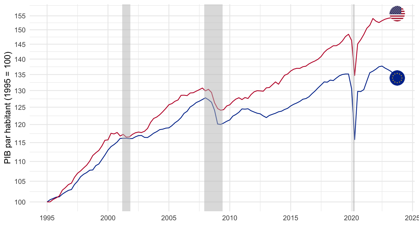

1996-

French

QNA %>%
  filter(LOCATION %in% c("USA", "EA20"),
         SUBJECT == "B1_GE",
         MEASURE == "VOBARSA",
         FREQUENCY == "Q") %>%
  quarter_to_date %>%
  left_join(QNA_var$LOCATION, by = "LOCATION") %>%
  select(LOCATION, Location, date, B1_GE_VOBARSA = obsValue) %>%
  left_join(SNA_TABLE3 %>%
              filter(TRANSACT == "POPNC",
                     MEASURE == "PER") %>%
              year_to_date %>%
              select(LOCATION, date, POPNC_PER = obsValue), 
            by = c("date", "LOCATION")) %>%
  filter(date >= as.Date("1996-01-01"),
         month(date) %% 3 == 1) %>%
  mutate(Location = ifelse(LOCATION == "EA20", "Europe", Location)) %>%
  select(Location, LOCATION, date, B1_GE_VOBARSA, POPNC_PER) %>%
  group_by(LOCATION) %>%
  mutate(POPNC_PER_i = spline(x = date, y = POPNC_PER, xout = date)$y,
         obsValue = B1_GE_VOBARSA/POPNC_PER_i) %>%
  arrange(date) %>%
  mutate(obsValue = 100 * obsValue / obsValue[date == as.Date("1996-01-01")]) %>%
  ggplot(.) + theme_minimal() + xlab("") + ylab("PIB par habitant (1996 = 100)") +
  geom_line(aes(x = date, y = obsValue, color = Location)) + add_2flags +
  geom_rect(data = nber_recessions %>%
              filter(Peak >= as.Date("1995-01-01")), 
            aes(xmin = Peak, xmax = Trough, ymin = 0, ymax = +Inf), 
            fill = 'grey', alpha = 0.5) +
  scale_color_manual(values = c("#003399", "#BF0A30")) +
  scale_x_date(breaks = seq(1960, 2025, 5) %>% paste0("-01-01") %>% as.Date,
               labels = date_format("%Y")) +
  theme(legend.position = "none") +
  scale_y_log10(breaks = seq(70, 200, 5))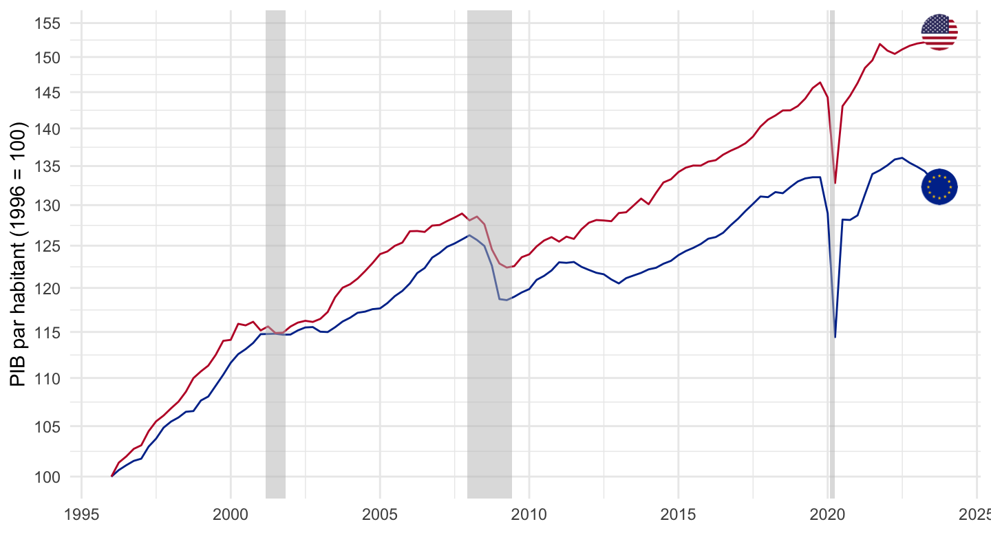

2000-

QNA %>%
  filter(LOCATION %in% c("USA", "EA20"),
         SUBJECT == "B1_GE",
         MEASURE == "VOBARSA",
         FREQUENCY == "Q") %>%
  quarter_to_date %>%
  select(LOCATION, date, B1_GE_VOBARSA = obsValue) %>%
  left_join(SNA_TABLE3 %>%
              filter(TRANSACT == "POPNC",
                     MEASURE == "PER") %>%
              year_to_date %>%
              select(LOCATION, date, POPNC_PER = obsValue), 
            by = c("date", "LOCATION")) %>%
  filter(date >= as.Date("1999-10-01"),
         month(date) %% 3 == 1) %>%
  mutate(date = date + months(3) -days(1)) %>%
  select(LOCATION, date, B1_GE_VOBARSA, POPNC_PER) %>%
  group_by(LOCATION) %>%
  mutate(POPNC_PER_i = spline(x = date, y = POPNC_PER, xout = date)$y,
         obsValue = B1_GE_VOBARSA/POPNC_PER_i) %>%
  left_join(QNA_var$LOCATION, by = "LOCATION") %>%
  mutate(Location = ifelse(LOCATION == "EA20", "Europe", Location)) %>%
  arrange(date) %>%
  mutate(obsValue = 100 * obsValue / obsValue[date == as.Date("2007-06-30")]) %>%
  left_join(colors, by = c("Location" = "country")) %>%
  mutate(color = ifelse(LOCATION == "USA", color2, color)) %>%
  ggplot(.) + theme_minimal() + xlab("") + ylab("GDP Per Capita (2007 = 100)") +
  geom_line(aes(x = date, y = obsValue, color = color)) +
  scale_color_identity() + add_2flags +
  geom_rect(data = nber_recessions %>%
              filter(Peak >= as.Date("1995-01-01")), 
            aes(xmin = Peak, xmax = Trough, ymin = 0, ymax = +Inf), 
            fill = 'grey', alpha = 0.5) +
  scale_x_date(breaks = seq(1960,2100,  2) %>% paste0("-01-01") %>% as.Date,
               labels = date_format("%Y")) +
  theme(legend.position = "none") +
  scale_y_log10(breaks = seq(70, 200, 2))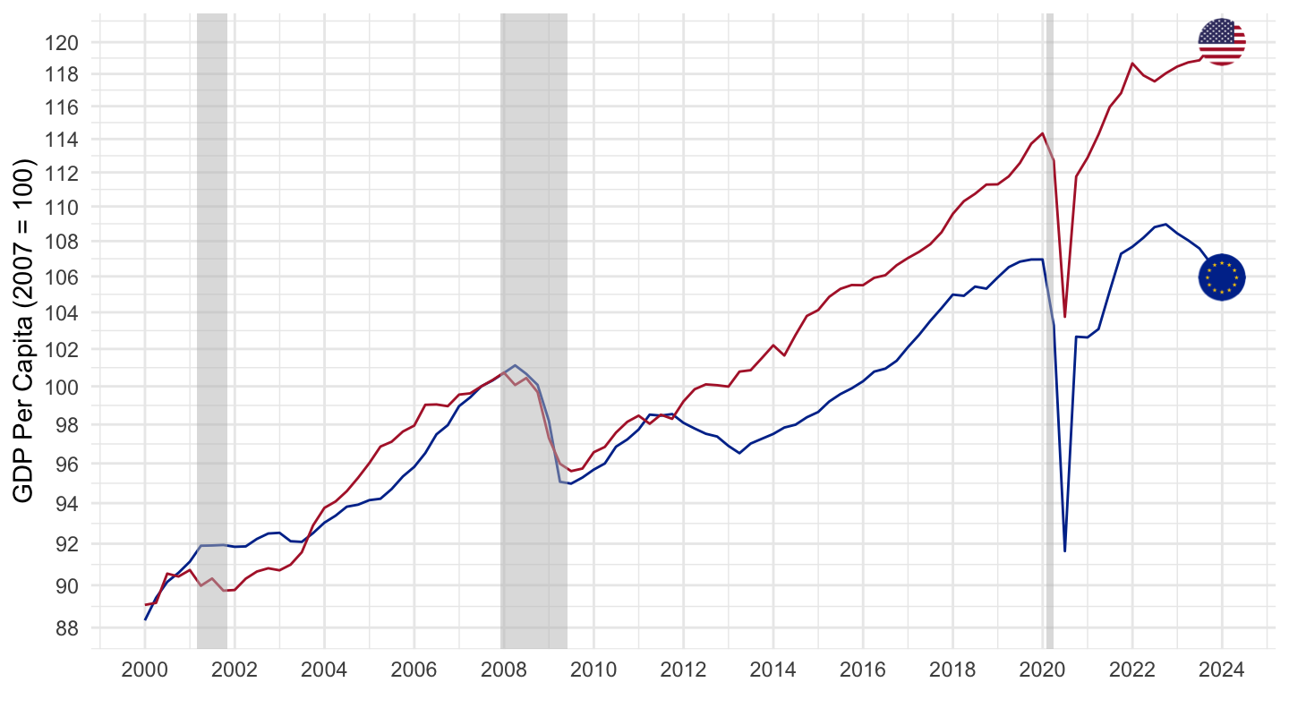

2015-

QNA %>%
  filter(LOCATION %in% c("USA", "EA20"),
         SUBJECT == "B1_GE",
         MEASURE == "VOBARSA",
         FREQUENCY == "Q") %>%
  quarter_to_date %>%
  select(LOCATION, date, B1_GE_VOBARSA = obsValue) %>%
  left_join(SNA_TABLE3 %>%
              filter(TRANSACT == "POPNC",
                     MEASURE == "PER") %>%
              year_to_date %>%
              select(LOCATION, date, POPNC_PER = obsValue), 
            by = c("date", "LOCATION")) %>%
  filter(date >= as.Date("2014-01-01"),
         month(date) %% 3 == 1) %>%
  select(LOCATION, date, B1_GE_VOBARSA, POPNC_PER) %>%
  group_by(LOCATION) %>%
  mutate(POPNC_PER_i = spline(x = date, y = POPNC_PER, xout = date)$y,
         obsValue = B1_GE_VOBARSA/POPNC_PER_i) %>%
  left_join(QNA_var$LOCATION, by = "LOCATION") %>%
  mutate(Location = ifelse(LOCATION == "EA20", "Europe", Location)) %>%
  arrange(date) %>%
  mutate(obsValue = 100 * obsValue / obsValue[date == as.Date("2014-01-01")]) %>%
  left_join(colors, by = c("Location" = "country")) %>%
  mutate(color = ifelse(LOCATION == "USA", color2, color)) %>%
  ggplot(.) + theme_minimal() + xlab("") + ylab("GDP Per Capita (2007 = 100)") +
  geom_line(aes(x = date, y = obsValue, color = color)) +
  scale_color_identity() + add_2flags +
  geom_rect(data = nber_recessions %>%
              filter(Peak >= as.Date("2015-01-01")),
            aes(xmin = Peak, xmax = Trough, ymin = 0, ymax = +Inf), 
            fill = 'grey', alpha = 0.5) +
  scale_y_log10(breaks = seq(70, 200, 2))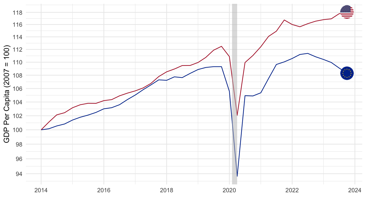

US, Europe, OECD

Tous

QNA %>%
  filter(LOCATION %in% c("USA", "EA20", "OECD"),
         SUBJECT == "B1_GE",
         MEASURE == "VPVOBARSA",
         FREQUENCY == "Q") %>%
  quarter_to_date %>%
  select(LOCATION, date, B1_GE_VOBARSA = obsValue) %>%
  left_join(SNA_TABLE3 %>%
              filter(TRANSACT == "POPNC",
                     MEASURE == "PER") %>%
              year_to_date %>%
              select(LOCATION, date, POPNC_PER = obsValue), 
            by = c("date", "LOCATION")) %>%
  filter(date >= as.Date("1999-10-01"),
         month(date) %% 3 == 1) %>%
  mutate(date = date + months(3) -days(1)) %>%
  select(LOCATION, date, B1_GE_VOBARSA, POPNC_PER) %>%
  group_by(LOCATION) %>%
  mutate(POPNC_PER_i = spline(x = date, y = POPNC_PER, xout = date)$y,
         obsValue = B1_GE_VOBARSA/POPNC_PER_i) %>%
  left_join(QNA_var$LOCATION, by = "LOCATION") %>%
  mutate(Location = ifelse(LOCATION == "EA20", "Europe", Location),
         Location = ifelse(LOCATION == "OECD", "OECD members", Location)) %>%
  arrange(date) %>%
  mutate(obsValue = 100 * obsValue / obsValue[date == as.Date("2007-06-30")]) %>%
  left_join(colors, by = c("Location" = "country")) %>%
  mutate(color = ifelse(LOCATION == "USA", color2, color)) %>%
  ggplot(.) + theme_minimal() + xlab("") + ylab("GDP Per Capita (2007 = 100)") +
  geom_line(aes(x = date, y = obsValue, color = color)) +
  scale_color_identity() + 
  geom_image(data = . %>%
               filter(date == as.Date("2021-12-31")) %>%
               mutate(image = paste0("../../icon/flag/round/", str_to_lower(gsub(" ", "-", Location)), ".png")),
             aes(x = date, y = obsValue, image = image), asp = 1.5) +
  geom_rect(data = nber_recessions %>%
              filter(Peak >= as.Date("1995-01-01")), 
            aes(xmin = Peak, xmax = Trough, ymin = 0, ymax = +Inf), 
            fill = 'grey', alpha = 0.5) +
  scale_x_date(breaks = seq(1960,2100,  2) %>% paste0("-01-01") %>% as.Date,
               labels = date_format("%Y")) +
  scale_y_log10(breaks = seq(70, 200, 2))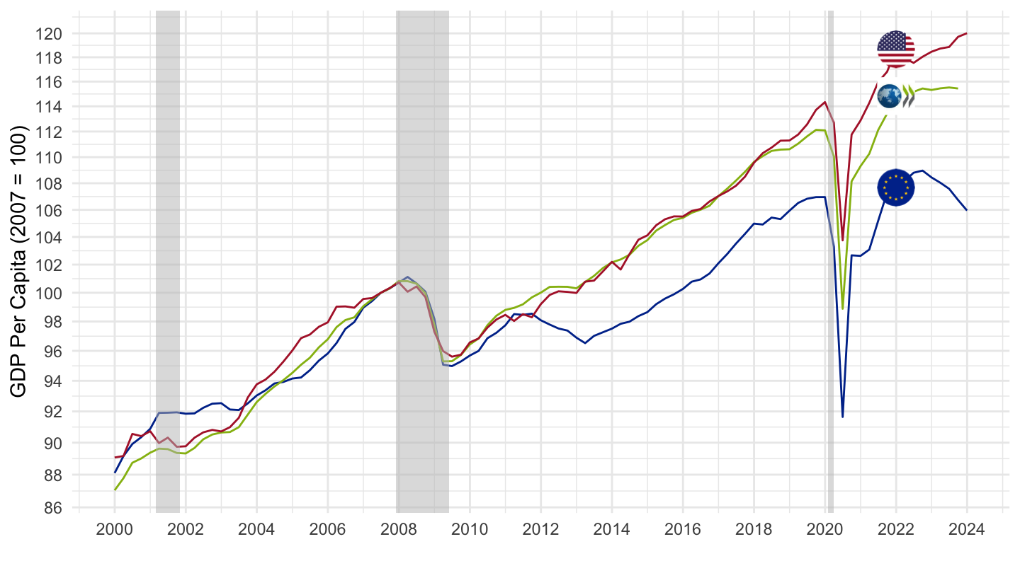

US, Europe, Italy

Tous

QNA %>%
  filter(LOCATION %in% c("USA", "EA20", "ITA"),
         SUBJECT == "B1_GE",
         MEASURE == "VOBARSA",
         FREQUENCY == "Q") %>%
  quarter_to_date %>%
  select(LOCATION, date, B1_GE_VOBARSA = obsValue) %>%
  left_join(SNA_TABLE3 %>%
              filter(TRANSACT == "POPNC",
                     MEASURE == "PER") %>%
              year_to_date %>%
              select(LOCATION, date, POPNC_PER = obsValue), 
            by = c("date", "LOCATION")) %>%
  filter(date >= as.Date("1999-10-01"),
         month(date) %% 3 == 1) %>%
  mutate(date = date + months(3) -days(1)) %>%
  select(LOCATION, date, B1_GE_VOBARSA, POPNC_PER) %>%
  group_by(LOCATION) %>%
  mutate(POPNC_PER_i = spline(x = date, y = POPNC_PER, xout = date)$y,
         obsValue = B1_GE_VOBARSA/POPNC_PER_i) %>%
  left_join(QNA_var$LOCATION, by = "LOCATION") %>%
  mutate(Location = ifelse(LOCATION == "EA20", "Europe", Location)) %>%
  arrange(date) %>%
  mutate(obsValue = 100 * obsValue / obsValue[date == as.Date("2007-06-30")]) %>%
  left_join(colors, by = c("Location" = "country")) %>%
  mutate(color = ifelse(LOCATION == "USA", color2, color)) %>%
  ggplot(.) + theme_minimal() + xlab("") + ylab("GDP Per Capita (2007 = 100)") +
  geom_line(aes(x = date, y = obsValue, color = color)) +
  scale_color_identity() + add_3flags +
  geom_rect(data = nber_recessions %>%
              filter(Peak >= as.Date("1995-01-01")), 
            aes(xmin = Peak, xmax = Trough, ymin = 0, ymax = +Inf), 
            fill = 'grey', alpha = 0.5) +
  scale_x_date(breaks = seq(1960,2100,  2) %>% paste0("-01-01") %>% as.Date,
               labels = date_format("%Y")) +
  scale_y_log10(breaks = seq(70, 200, 2))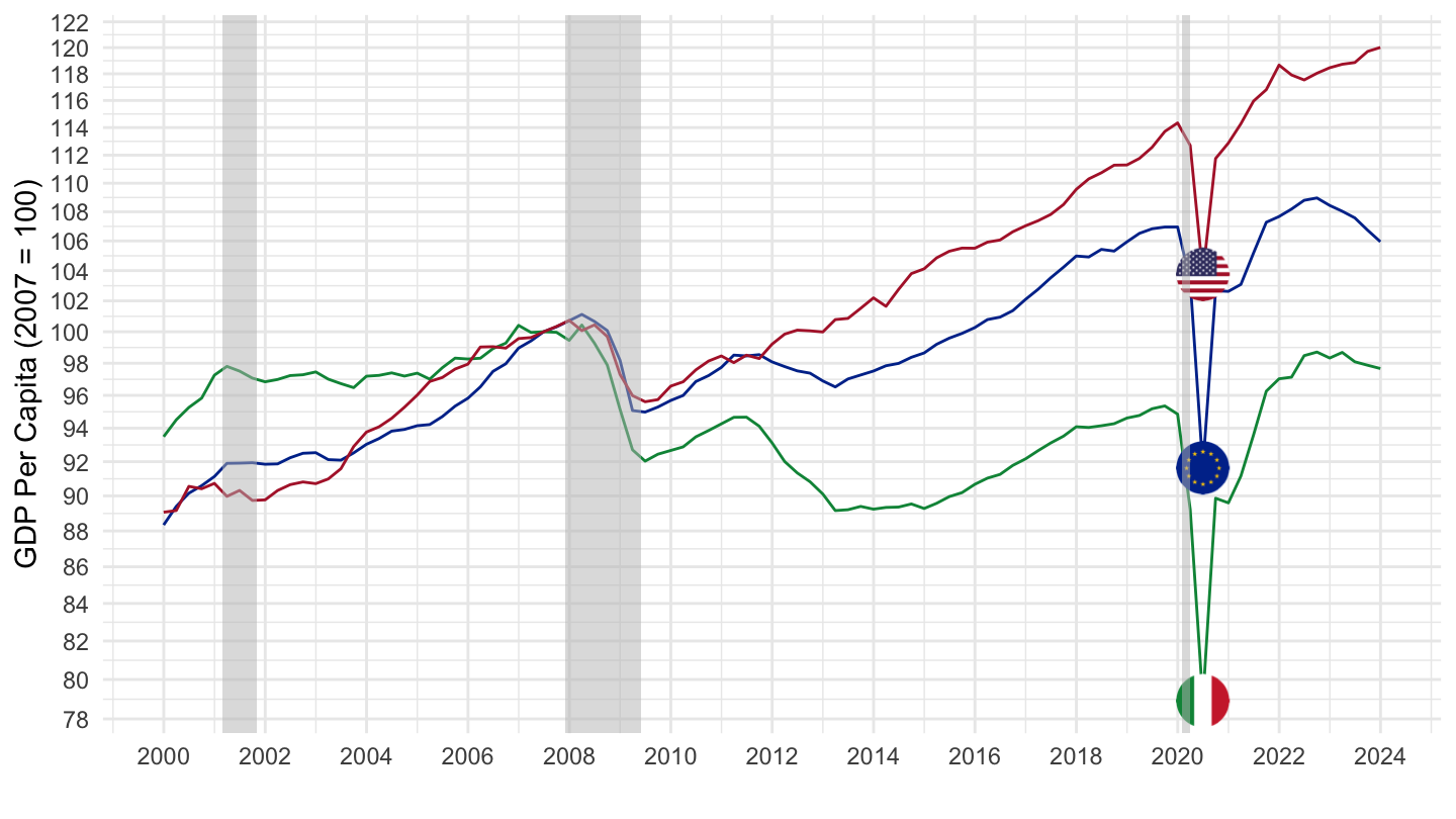

1995-

English

QNA %>%
  filter(LOCATION %in% c("USA", "EA20", "ITA"),
         SUBJECT == "B1_GE",
         MEASURE == "VOBARSA",
         FREQUENCY == "Q") %>%
  quarter_to_date %>%
  select(LOCATION, date, B1_GE_VOBARSA = obsValue) %>%
  left_join(SNA_TABLE3 %>%
              filter(TRANSACT == "POPNC",
                     MEASURE == "PER") %>%
              year_to_date %>%
              select(LOCATION, date, POPNC_PER = obsValue), 
            by = c("date", "LOCATION")) %>%
  filter(date >= as.Date("1995-01-01"),
         month(date) %% 3 == 1) %>%
  select(LOCATION, date, B1_GE_VOBARSA, POPNC_PER) %>%
  group_by(LOCATION) %>%
  mutate(POPNC_PER_i = spline(x = date, y = POPNC_PER, xout = date)$y,
         obsValue = B1_GE_VOBARSA/POPNC_PER_i) %>%
  left_join(QNA_var$LOCATION, by = "LOCATION") %>%
  arrange(date) %>%
  mutate(obsValue = 100 * obsValue / obsValue[date == as.Date("1995-01-01")]) %>%
  mutate(Location = ifelse(LOCATION == "EA20", "Europe", Location)) %>%
  left_join(colors, by = c("Location" = "country")) %>%
  mutate(color = ifelse(LOCATION == "USA", color2, color)) %>%
  ggplot(.) + theme_minimal() + xlab("") + ylab("GDP Per Capita (1995 = 100)") +
  geom_line(aes(x = date, y = obsValue, color = color)) +
  scale_color_identity() + add_3flags +
  geom_rect(data = nber_recessions %>%
              filter(Peak >= as.Date("1995-01-01")), 
            aes(xmin = Peak, xmax = Trough, ymin = 0, ymax = +Inf), 
            fill = 'grey', alpha = 0.5) +
  scale_x_date(breaks = seq(1960, 2022, 5) %>% paste0("-01-01") %>% as.Date,
               labels = date_format("%Y")) +
  scale_y_log10(breaks = seq(70, 200, 5))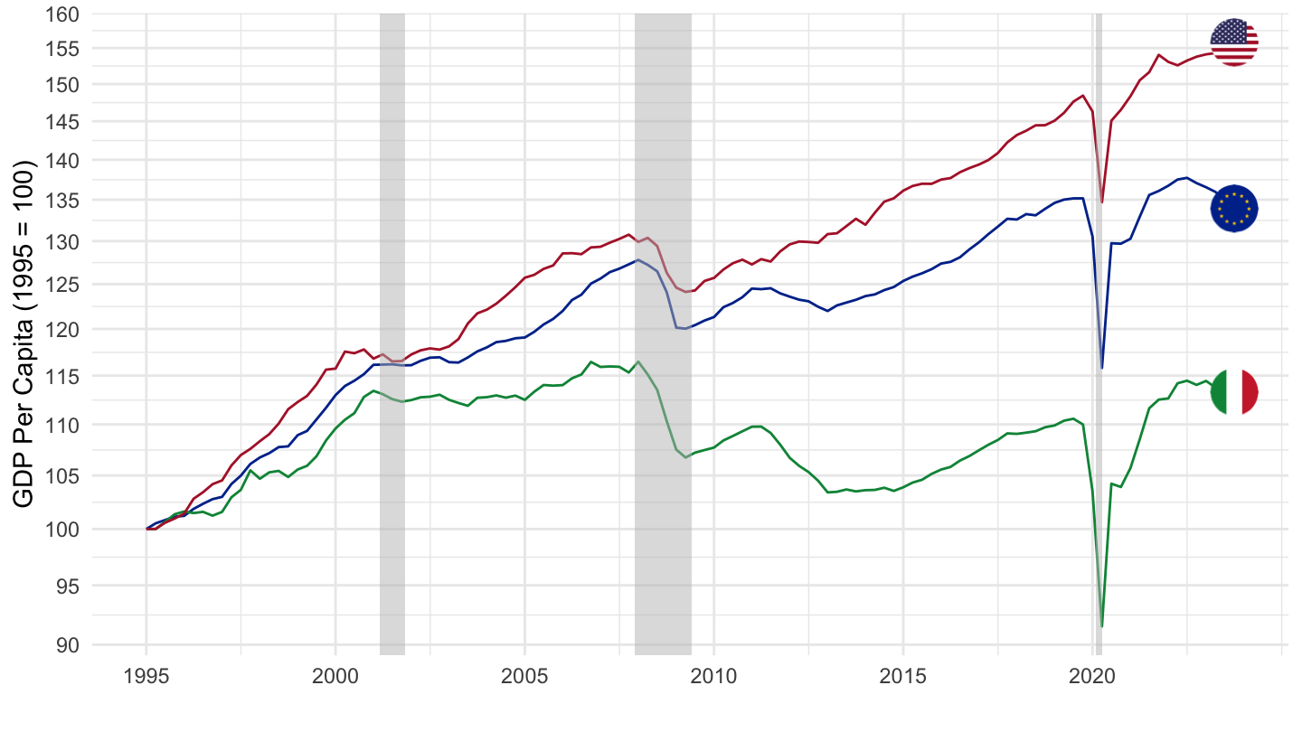

French

QNA %>%
  filter(LOCATION %in% c("USA", "EA20", "ITA"),
         SUBJECT == "B1_GE",
         MEASURE == "VOBARSA",
         FREQUENCY == "Q") %>%
  quarter_to_date %>%
  select(LOCATION, date, B1_GE_VOBARSA = obsValue) %>%
  left_join(SNA_TABLE3 %>%
              filter(TRANSACT == "POPNC",
                     MEASURE == "PER") %>%
              year_to_date %>%
              select(LOCATION, date, POPNC_PER = obsValue), 
            by = c("date", "LOCATION")) %>%
  filter(date >= as.Date("1995-01-01"),
         month(date) %% 3 == 1) %>%
  select(LOCATION, date, B1_GE_VOBARSA, POPNC_PER) %>%
  group_by(LOCATION) %>%
  mutate(POPNC_PER_i = spline(x = date, y = POPNC_PER, xout = date)$y,
         obsValue = B1_GE_VOBARSA/POPNC_PER_i) %>%
  left_join(QNA_var$LOCATION, by = "LOCATION") %>%
  arrange(date) %>%
  mutate(obsValue = 100 * obsValue / obsValue[date == as.Date("1995-01-01")]) %>%
  mutate(Location = ifelse(LOCATION == "EA20", "Europe", Location)) %>%
  left_join(colors, by = c("Location" = "country")) %>%
  mutate(color = ifelse(LOCATION == "USA", color2, color)) %>%
  ggplot(.) + theme_minimal() + xlab("") + ylab("PIB par habitant (1995=100)") +
  geom_line(aes(x = date, y = obsValue, color = color)) +
  scale_color_identity() + add_3flags +
  geom_rect(data = nber_recessions %>%
              filter(Peak >= as.Date("1995-01-01")), 
            aes(xmin = Peak, xmax = Trough, ymin = 0, ymax = +Inf), 
            fill = 'grey', alpha = 0.5) +
  scale_x_date(breaks = seq(1960, 2022, 5) %>% paste0("-01-01") %>% as.Date,
               labels = date_format("%Y")) +
  scale_y_log10(breaks = seq(70, 200, 5))

Europe VS Japan

100 = 2003

QNA %>%
  filter(LOCATION %in% c("JPN", "EA20"),
         SUBJECT == "B1_GE",
         MEASURE == "VOBARSA",
         FREQUENCY == "Q") %>%
  quarter_to_date %>%
  left_join(QNA_var$LOCATION, by = "LOCATION") %>%
  select(LOCATION,  Location, date, B1_GE_VOBARSA = obsValue) %>%
  left_join(SNA_TABLE3 %>%
              filter(TRANSACT == "POPNC",
                     MEASURE == "PER") %>%
              year_to_date %>%
              select(LOCATION, date, POPNC_PER = obsValue), 
            by = c("date", "LOCATION")) %>%
  filter(date >= as.Date("1999-10-01"),
         month(date) %% 3 == 1) %>%
  mutate(date = date + months(3) -days(1)) %>%
  select(LOCATION, Location, date, B1_GE_VOBARSA, POPNC_PER) %>%
  mutate(Location = ifelse(LOCATION == "EA20", "Europe", Location)) %>%
  group_by(Location) %>%
  mutate(POPNC_PER_i = spline(x = date, y = POPNC_PER, xout = date)$y,
         obsValue = B1_GE_VOBARSA/POPNC_PER_i) %>%
  arrange(date) %>%
  mutate(obsValue = 100 * obsValue / obsValue[date == as.Date("2002-12-31")]) %>%
  ggplot(.) + theme_minimal() + xlab("") + ylab("GDP Per Capita (2003 = 100)") +
  geom_line(aes(x = date, y = obsValue, color = Location)) +
  geom_image(data = . %>%
               filter(date == as.Date("2013-12-31")) %>%
               mutate(image = paste0("../../icon/flag/round/", str_to_lower(gsub(" ", "-", Location)), ".png")),
             aes(x = date, y = obsValue, image = image), asp = 1.5) +
  geom_rect(data = nber_recessions %>%
              filter(Peak >= as.Date("1995-01-01")), 
            aes(xmin = Peak, xmax = Trough, ymin = 0, ymax = +Inf), 
            fill = 'grey', alpha = 0.5) +
  scale_color_manual(values = c("#003399", "#be0029")) +
  scale_x_date(breaks = seq(1960,2100,  2) %>% paste0("-01-01") %>% as.Date,
               labels = date_format("%Y")) +
  theme(legend.position = "none") +
  scale_y_log10(breaks = seq(70, 200, 2))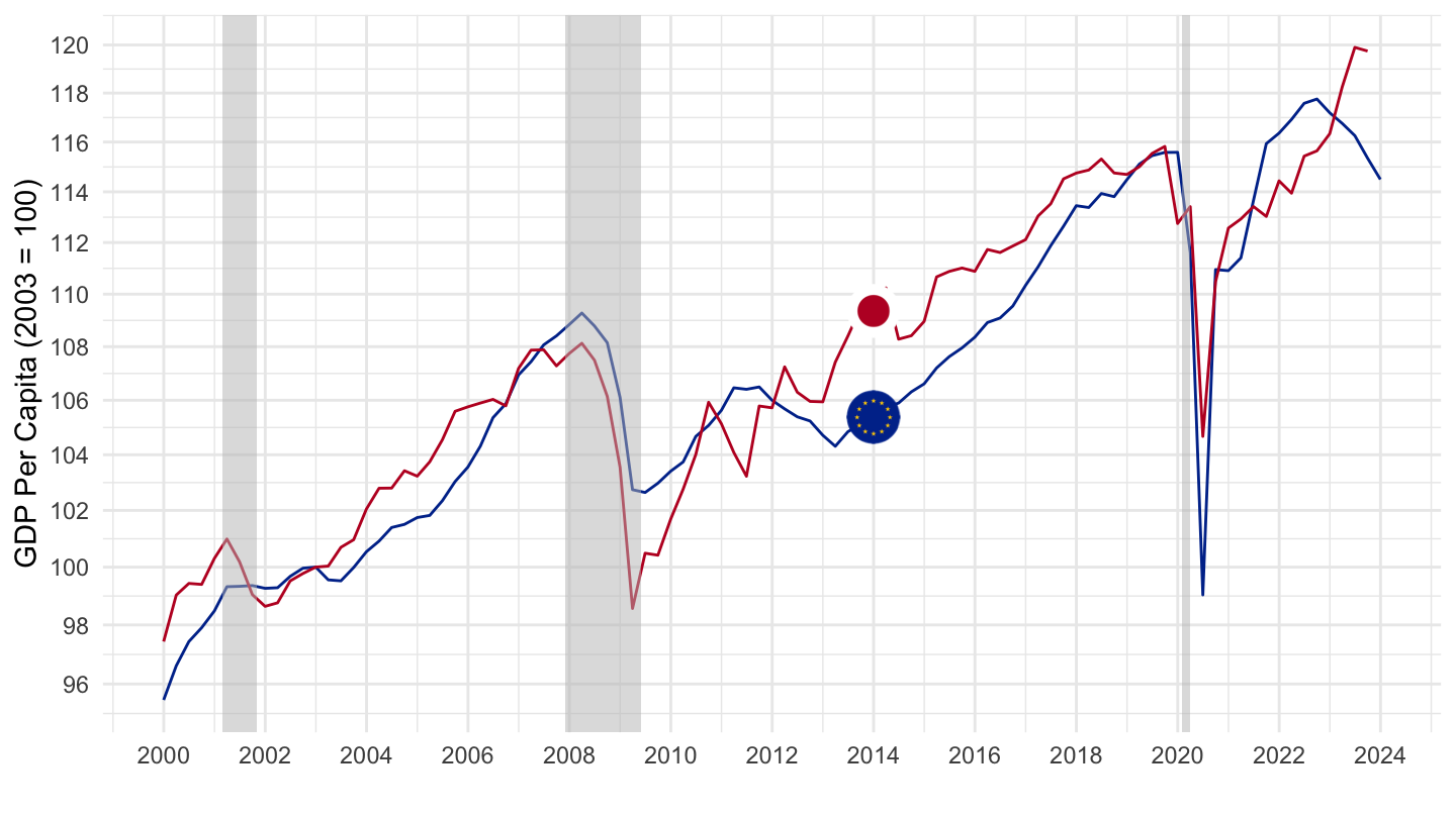

100 = 2000

QNA %>%
  filter(LOCATION %in% c("JPN", "EA20"),
         SUBJECT == "B1_GE",
         MEASURE == "VOBARSA",
         FREQUENCY == "Q") %>%
  quarter_to_date %>%
  select(LOCATION, date, B1_GE_VOBARSA = obsValue) %>%
  left_join(SNA_TABLE3 %>%
              filter(TRANSACT == "POPNC",
                     MEASURE == "PER") %>%
              year_to_date %>%
              select(LOCATION, date, POPNC_PER = obsValue), 
            by = c("date", "LOCATION")) %>%
  filter(date >= as.Date("2000-01-01")) %>%
  select(LOCATION, date, B1_GE_VOBARSA, POPNC_PER) %>%
  group_by(LOCATION) %>%
  mutate(POPNC_PER_i = spline(x = date, y = POPNC_PER, xout = date)$y,
         obsValue = B1_GE_VOBARSA/POPNC_PER_i,
         Location = case_when(LOCATION == "JPN" ~ "Japan",
                              LOCATION == "EA20" ~ "Europe",
                              LOCATION == "ITA" ~ "Italy")) %>%
  arrange(date) %>%
  mutate(obsValue = 100 * obsValue / obsValue[date == as.Date("2000-01-01")]) %>%
  ggplot(.) + theme_minimal() + xlab("") + ylab("GDP Per Capita (2001 = 100)") +
  geom_line(aes(x = date, y = obsValue, color = LOCATION)) +
  geom_image(data = . %>%
               filter(date == as.Date("2011-01-01")) %>%
               mutate(image = paste0("../../icon/flag/round/", str_to_lower(gsub(" ", "-", Location)), ".png")),
             aes(x = date, y = obsValue, image = image), asp = 1.5) +
  scale_color_manual(values = c("#003399", "#be0029")) +
  scale_x_date(breaks = seq(1960,2100,  2) %>% paste0("-01-01") %>% as.Date,
               labels = date_format("%Y")) +
  theme(legend.position = "none") +
  scale_y_log10(breaks = seq(70, 200, 2))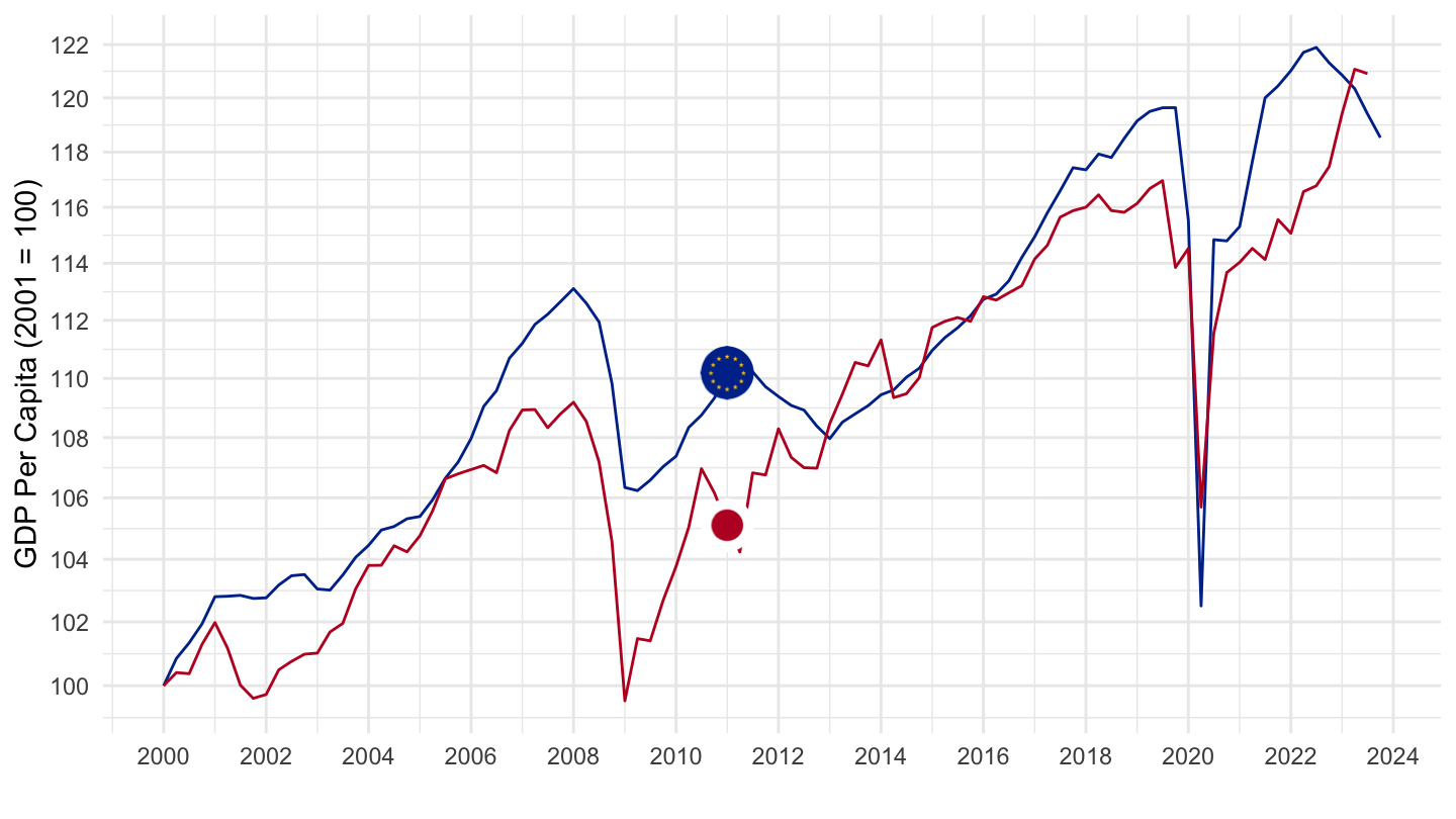

100 = 1995

QNA %>%
  filter(LOCATION %in% c("JPN", "EA20"),
         SUBJECT == "B1_GE",
         MEASURE == "VOBARSA",
         FREQUENCY == "Q") %>%
  quarter_to_date %>%
  select(LOCATION, date, B1_GE_VOBARSA = obsValue) %>%
  left_join(SNA_TABLE3 %>%
              filter(TRANSACT == "POPNC",
                     MEASURE == "PER") %>%
              year_to_date %>%
              select(LOCATION, date, POPNC_PER = obsValue), 
            by = c("date", "LOCATION")) %>%
  filter(date >= as.Date("1995-01-01")) %>%
  select(LOCATION, date, B1_GE_VOBARSA, POPNC_PER) %>%
  group_by(LOCATION) %>%
  mutate(POPNC_PER_i = spline(x = date, y = POPNC_PER, xout = date)$y,
         obsValue = B1_GE_VOBARSA/POPNC_PER_i,
         Location = case_when(LOCATION == "JPN" ~ "Japan",
                              LOCATION == "EA20" ~ "Europe",
                              LOCATION == "ITA" ~ "Italy")) %>%
  arrange(date) %>%
  mutate(obsValue = 100 * obsValue / obsValue[date == as.Date("1995-01-01")]) %>%
  ggplot(.) + theme_minimal() + xlab("") + ylab("GDP Per Capita (2001 = 100)") +
  geom_line(aes(x = date, y = obsValue, color = LOCATION)) +
  geom_image(data = . %>%
               filter(date == as.Date("2016-01-01")) %>%
               mutate(image = paste0("../../icon/flag/round/", str_to_lower(gsub(" ", "-", Location)), ".png")),
             aes(x = date, y = obsValue, image = image), asp = 1.5) +
  scale_color_manual(values = c("#003399", "#be0029")) +
  scale_x_date(breaks = seq(1960,2100,  2) %>% paste0("-01-01") %>% as.Date,
               labels = date_format("%Y")) +
  theme(legend.position = "none",
        legend.title = element_blank()) +
  scale_y_log10(breaks = seq(70, 200, 2))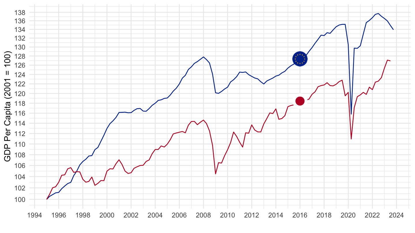

US VS Europe VS Sweden

Ex 1

QNA %>%
  filter(LOCATION %in% c("USA", "SWE"),
         SUBJECT == "B1_GE",
         MEASURE == "VOBARSA",
         FREQUENCY == "Q") %>%
  quarter_to_date %>%
  left_join(QNA_var$LOCATION, by = "LOCATION") %>%
  select(LOCATION, Location, date, B1_GE_VOBARSA = obsValue) %>%
  left_join(SNA_TABLE3 %>%
              filter(TRANSACT == "POPNC",
                     MEASURE == "PER") %>%
              year_to_date %>%
              select(LOCATION, date, POPNC_PER = obsValue), 
            by = c("date", "LOCATION")) %>%
  filter(date >= as.Date("1980-10-01"),
         date <= as.Date("2006-01-01"),
         month(date) %% 3 == 1) %>%
  mutate(date = date + months(3) -days(1)) %>%
  mutate(Location = ifelse(LOCATION == "EA20", "Europe", Location)) %>%
  select(Location, LOCATION, date, B1_GE_VOBARSA, POPNC_PER) %>%
  group_by(LOCATION) %>%
  mutate(POPNC_PER_i = spline(x = date, y = POPNC_PER, xout = date)$y,
         obsValue = B1_GE_VOBARSA/POPNC_PER_i) %>%
  arrange(date) %>%
  mutate(obsValue = 100 * obsValue / obsValue[date == as.Date("1990-06-30")]) %>%
  ggplot(.) + theme_minimal() + xlab("") + ylab("GDP Per Capita (2007 = 100)") +
  geom_line(aes(x = date, y = obsValue, color = Location)) +
  geom_image(data = . %>%
               filter(date == as.Date("2000-12-31")) %>%
               mutate(image = paste0("../../icon/flag/round/", str_to_lower(gsub(" ", "-", Location)), ".png")),
             aes(x = date, y = obsValue, image = image), asp = 1.5) +
  geom_rect(data = nber_recessions %>%
              filter(Peak >= as.Date("1995-01-01")), 
            aes(xmin = Peak, xmax = Trough, ymin = 0, ymax = +Inf), 
            fill = 'grey', alpha = 0.5) +
  scale_color_manual(values = c("#003399", "#BF0A30")) +
  scale_x_date(breaks = seq(1960,2100,  2) %>% paste0("-01-01") %>% as.Date,
               labels = date_format("%Y")) +
  theme(legend.position = "none") +
  scale_y_log10(breaks = seq(70, 200, 2))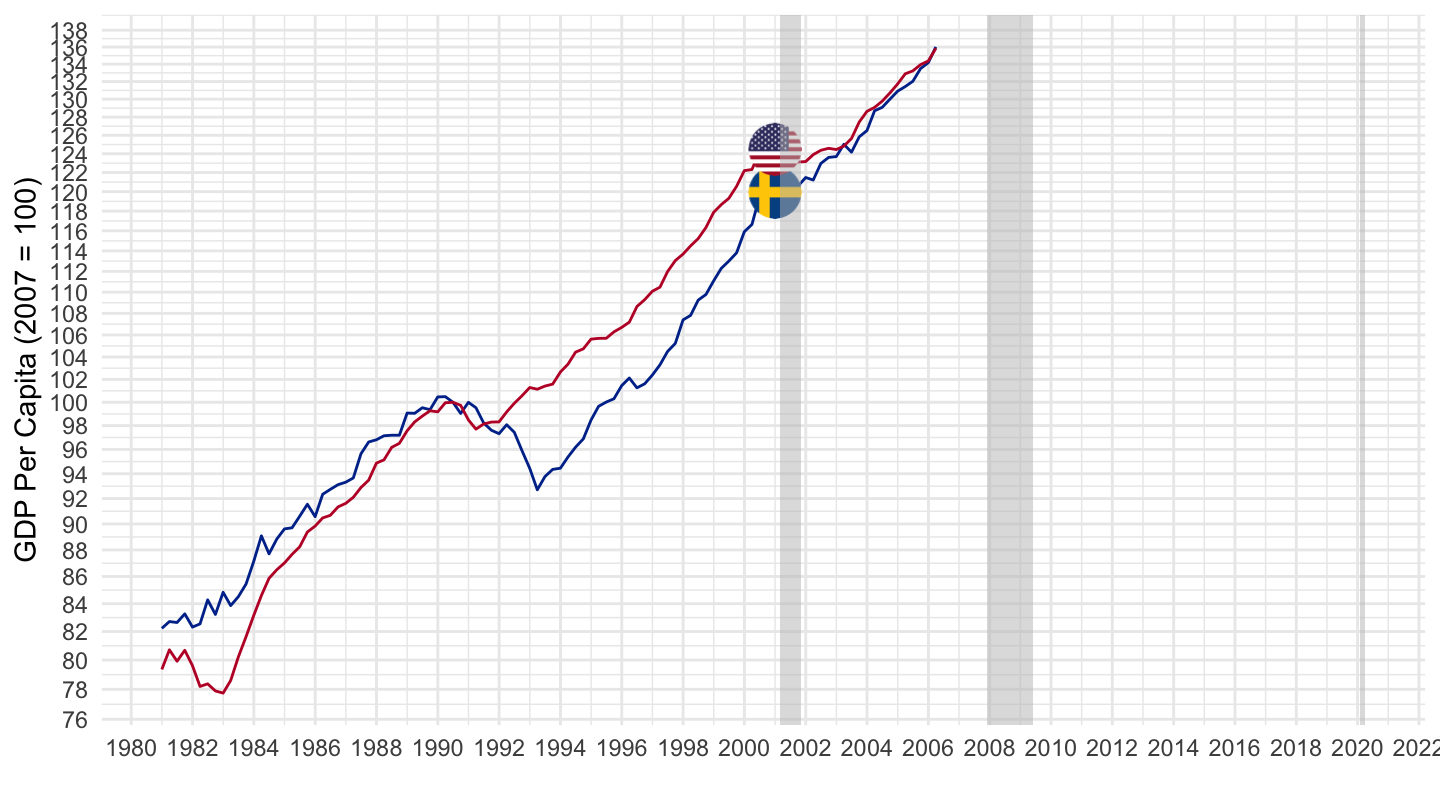

France, Italy, Europe, US, Germany

Base 100

1995-

VOBARSA

QNA %>%
  filter(LOCATION %in% c("USA", "EA20", "ITA", "FRA", "DEU"),
         SUBJECT == "B1_GE",
         MEASURE == "VOBARSA",
         FREQUENCY == "Q") %>%
  quarter_to_date %>%
  select(LOCATION, date, B1_GE_VOBARSA = obsValue) %>%
  left_join(SNA_TABLE3 %>%
              filter(TRANSACT == "POPNC",
                     MEASURE == "PER") %>%
              year_to_date %>%
              select(LOCATION, date, POPNC_PER = obsValue), 
            by = c("date", "LOCATION")) %>%
  filter(date >= as.Date("1995-01-01"),
         month(date) %% 3 == 1) %>%
  select(LOCATION, date, B1_GE_VOBARSA, POPNC_PER) %>%
  group_by(LOCATION) %>%
  mutate(POPNC_PER_i = spline(x = date, y = POPNC_PER, xout = date)$y,
         obsValue = B1_GE_VOBARSA/POPNC_PER_i) %>%
  left_join(QNA_var$LOCATION, by = "LOCATION") %>%
  arrange(date) %>%
  mutate(obsValue = 100 * obsValue / obsValue[date == as.Date("1995-01-01")]) %>%
  mutate(Location = ifelse(LOCATION == "EA20", "Europe", Location)) %>%
  left_join(colors, by = c("Location" = "country")) %>%
  mutate(color = ifelse(LOCATION == "USA", color2, color),
         color = ifelse(LOCATION == "EA20", color2, color)) %>%
  ggplot(.) + theme_minimal() + xlab("") + ylab("PIB par habitant (1995 = 100)") +
  geom_line(aes(x = date, y = obsValue, color = color)) +
  scale_color_identity() + 
  geom_image(data = . %>%
               filter(date == as.Date("2017-01-01")) %>%
               mutate(image = paste0("../../icon/flag/round/", str_to_lower(gsub(" ", "-", Location)), ".png")),
             aes(x = date, y = obsValue, image = image), asp = 1.5) +
  geom_rect(data = nber_recessions %>%
              filter(Peak >= as.Date("1995-01-01")), 
            aes(xmin = Peak, xmax = Trough, ymin = 0, ymax = +Inf), 
            fill = 'grey', alpha = 0.5) +
  scale_x_date(breaks = seq(1960, 2022, 5) %>% paste0("-01-01") %>% as.Date,
               labels = date_format("%Y")) +
  scale_y_log10(breaks = seq(70, 200, 5))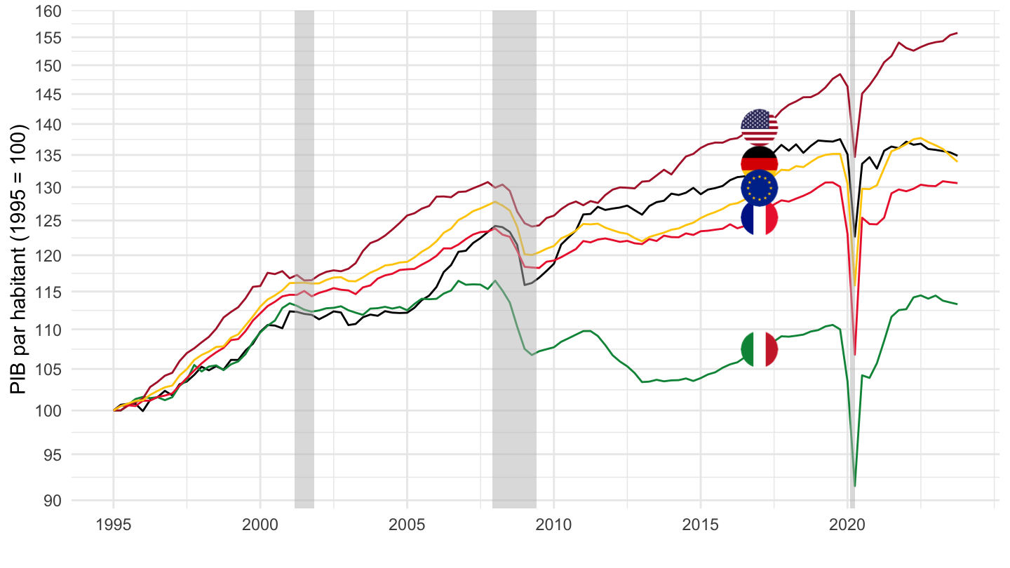

VOBARSA

QNA %>%
  filter(LOCATION %in% c("USA", "EA20", "ITA", "FRA", "DEU"),
         SUBJECT == "B1_GE",
         MEASURE == "VOBARSA",
         FREQUENCY == "Q") %>%
  quarter_to_date %>%
  select(LOCATION, date, B1_GE_VOBARSA = obsValue) %>%
  left_join(SNA_TABLE3 %>%
              filter(TRANSACT == "POPNC",
                     MEASURE == "PER") %>%
              year_to_date %>%
              select(LOCATION, date, POPNC_PER = obsValue), 
            by = c("date", "LOCATION")) %>%
  filter(date >= as.Date("1995-01-01"),
         month(date) %% 3 == 1) %>%
  select(LOCATION, date, B1_GE_VOBARSA, POPNC_PER) %>%
  group_by(LOCATION) %>%
  mutate(POPNC_PER_i = spline(x = date, y = POPNC_PER, xout = date)$y,
         obsValue = B1_GE_VOBARSA/POPNC_PER_i) %>%
  left_join(QNA_var$LOCATION, by = "LOCATION") %>%
  arrange(date) %>%
  mutate(obsValue = 100 * obsValue / obsValue[date == as.Date("1995-01-01")]) %>%
  mutate(Location = ifelse(LOCATION == "EA20", "Europe", Location)) %>%
  left_join(colors, by = c("Location" = "country")) %>%
  mutate(color = ifelse(LOCATION == "USA", color2, color),
         color = ifelse(LOCATION == "EA20", color2, color)) %>%
  ggplot(.) + theme_minimal() + xlab("") + ylab("PIB par habitant (1995 = 100)") +
  geom_line(aes(x = date, y = obsValue, color = color)) +
  scale_color_identity() + add_5flags +
  geom_rect(data = nber_recessions %>%
              filter(Peak >= as.Date("1995-01-01")), 
            aes(xmin = Peak, xmax = Trough, ymin = 0, ymax = +Inf), 
            fill = 'grey', alpha = 0.5) +
  scale_x_date(breaks = seq(1960, 2022, 5) %>% paste0("-01-01") %>% as.Date,
               labels = date_format("%Y")) +
  scale_y_log10(breaks = seq(70, 200, 5))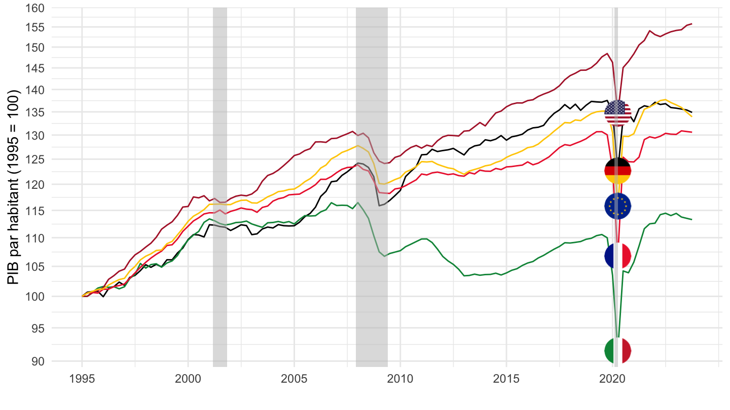

GDP

CPCARSA - US dollars, current prices, current PPPs, annual levels, seasonally adjusted

QNA %>%
  filter(SUBJECT == "B1_GE",
         MEASURE == "CPCARSA",
         FREQUENCY == "Q") %>%
  left_join(QNA_var$LOCATION, by = "LOCATION") %>%
  group_by(LOCATION, Location) %>%
  summarise(obsTime = last(obsTime),
            obsValue = last(obsValue)) %>%
  arrange(-obsValue) %>%
  mutate(Flag = gsub(" ", "-", str_to_lower(Location)),
         Flag = paste0('<img src="../../icon/flag/vsmall/', Flag, '.png" alt="Flag">')) %>%
  select(Flag, everything()) %>%
  {if (is_html_output()) datatable(., filter = 'top', rownames = F, escape = F) else .}

VPVOBARSA - US dollars, volume estimates, fixed PPPs (2015), OECD reference year, annual levels, seasonally adjusted

QNA %>%
  filter(SUBJECT == "B1_GE",
         MEASURE == "CPCARSA",
         FREQUENCY == "Q") %>%
  left_join(QNA_var$LOCATION, by = "LOCATION") %>%
  group_by(LOCATION, Location) %>%
  summarise(obsTime = last(obsTime),
            obsValue = last(obsValue)) %>%
  arrange(-obsValue) %>%
  mutate(Flag = gsub(" ", "-", str_to_lower(Location)),
         Flag = paste0('<img src="../../icon/flag/vsmall/', Flag, '.png" alt="Flag">')) %>%
  select(Flag, everything()) %>%
  {if (is_html_output()) datatable(., filter = 'top', rownames = F, escape = F) else .}

France, Germany, Italy, Spain, United States

1992-

QNA %>%
  filter(LOCATION %in% c("FRA", "DEU", "ITA", "ESP", "USA"),
         SUBJECT == "B1_GE",
         MEASURE == "VOBARSA",
         FREQUENCY == "Q") %>%
  quarter_to_date %>%
  filter(date >= as.Date("1992-01-01")) %>%
  left_join(QNA_var$LOCATION, by = "LOCATION") %>%
  mutate(Location = ifelse(LOCATION == "EA20", "Europe", Location)) %>%
  group_by(LOCATION) %>%
  mutate(obsValue = 100 * obsValue / obsValue[date == as.Date("1992-01-01")]) %>%
  left_join(colors, by = c("Location" = "country")) %>%
  mutate(color = ifelse(LOCATION == "USA", color2, color)) %>%
  ggplot(.) + theme_minimal() + xlab("") + ylab("GDP, Real (1992 = 100)") +
  geom_line(aes(x = date, y = obsValue, color = color)) +
  scale_color_identity() + add_5flags +
  geom_rect(data = nber_recessions %>%
              filter(Peak >= as.Date("1995-01-01")), 
            aes(xmin = Peak, xmax = Trough, ymin = 0, ymax = +Inf), 
            fill = 'grey', alpha = 0.5) +
  scale_x_date(breaks = seq(1960,2100,  2) %>% paste0("-01-01") %>% as.Date,
               labels = date_format("%Y")) +
  scale_y_log10(breaks = seq(70, 200, 5))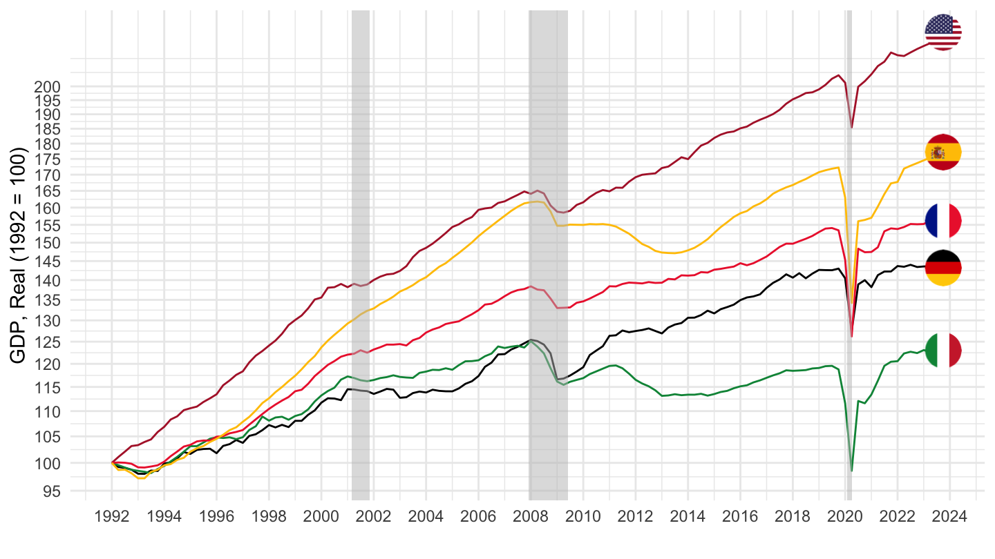

1996-

QNA %>%
  filter(LOCATION %in% c("FRA", "DEU", "ITA", "ESP", "USA"),
         SUBJECT == "B1_GE",
         MEASURE == "VOBARSA",
         FREQUENCY == "Q") %>%
  quarter_to_date %>%
  filter(date >= as.Date("1996-01-01")) %>%
  left_join(QNA_var$LOCATION, by = "LOCATION") %>%
  mutate(Location = ifelse(LOCATION == "EA20", "Europe", Location)) %>%
  group_by(LOCATION) %>%
  mutate(obsValue = 100 * obsValue / obsValue[date == as.Date("1996-01-01")]) %>%
  left_join(colors, by = c("Location" = "country")) %>%
  mutate(color = ifelse(LOCATION == "USA", color2, color)) %>%
  ggplot(.) + theme_minimal() + xlab("") + ylab("GDP, Real (1996 = 100)") +
  geom_line(aes(x = date, y = obsValue, color = color)) +
  scale_color_identity() + add_5flags +
  geom_rect(data = nber_recessions %>%
              filter(Peak >= as.Date("1995-01-01")), 
            aes(xmin = Peak, xmax = Trough, ymin = 0, ymax = +Inf), 
            fill = 'grey', alpha = 0.5) +
  scale_x_date(breaks = seq(1960,2100,  2) %>% paste0("-01-01") %>% as.Date,
               labels = date_format("%Y")) +
  scale_y_log10(breaks = seq(70, 200, 5))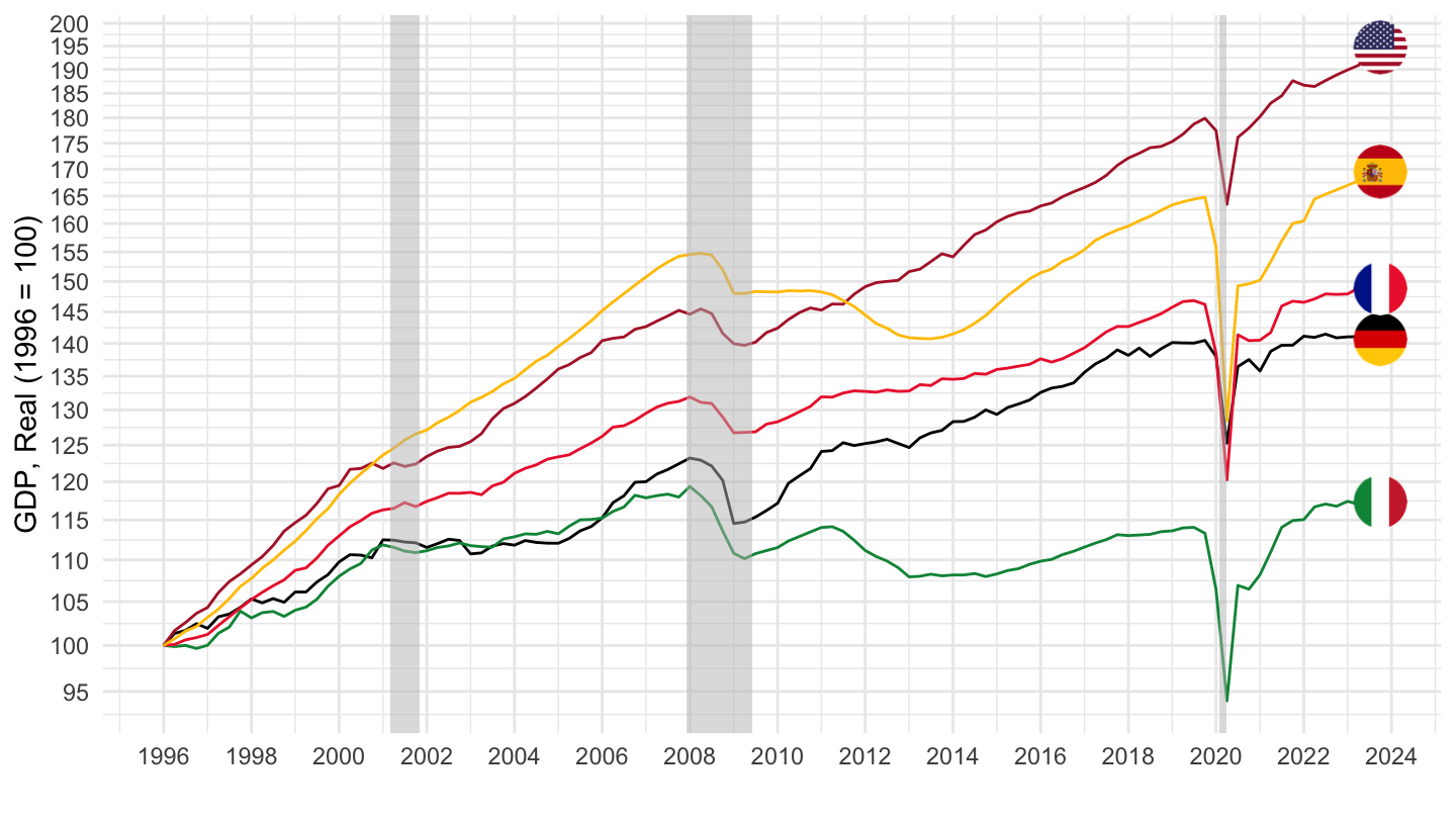

EU, France, Germany, US

1995-

QNA %>%
  filter(LOCATION %in% c("USA", "EA20", "FRA", "DEU"),
         SUBJECT == "B1_GE",
         MEASURE == "VOBARSA",
         FREQUENCY == "Q") %>%
  quarter_to_date %>%
  filter(date >= as.Date("1995-01-01")) %>%
  left_join(QNA_var$LOCATION, by = "LOCATION") %>%
  mutate(Location = ifelse(LOCATION == "EA20", "Europe", Location)) %>%
  arrange(date) %>%
  mutate(obsValue = 100 * obsValue / obsValue[date == as.Date("1995-01-01")]) %>%
  left_join(colors, by = c("Location" = "country")) %>%
  mutate(color = ifelse(LOCATION == "USA", color2, color),
         color = ifelse(LOCATION == "EA20", color2, color)) %>%
  ggplot(.) + theme_minimal() + xlab("") + ylab("GDP, Real (1995 = 100)") +
  geom_line(aes(x = date, y = obsValue, color = color)) +
  scale_color_identity() + add_4flags +
  geom_rect(data = nber_recessions %>%
              filter(Peak >= as.Date("1995-01-01")), 
            aes(xmin = Peak, xmax = Trough, ymin = 0, ymax = +Inf), 
            fill = 'grey', alpha = 0.5) +
  scale_x_date(breaks = seq(1960, 2022, 5) %>% paste0("-01-01") %>% as.Date,
               labels = date_format("%Y")) +
  scale_y_log10(breaks = seq(70, 200, 5))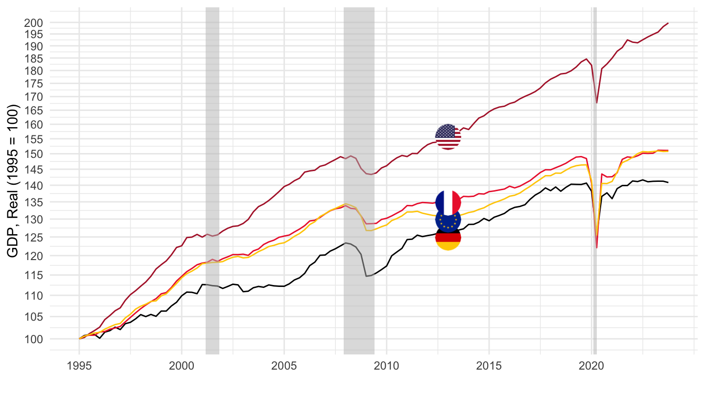

EU, France, Germany, US, Japan

1995-

QNA %>%
  filter(LOCATION %in% c("USA", "EA20", "FRA", "DEU", "OECD"),
         SUBJECT == "B1_GE",
         MEASURE == "VPVOBARSA",
         FREQUENCY == "Q") %>%
  quarter_to_date %>%
  filter(date >= as.Date("1995-01-01")) %>%
  left_join(QNA_var$LOCATION, by = "LOCATION") %>%
  mutate(Location = ifelse(LOCATION == "EA20", "Europe", Location),
         Location = ifelse(LOCATION == "OECD", "OECD members", Location)) %>%
  arrange(date) %>%
  group_by(Location) %>%
  mutate(obsValue = 100 * obsValue / obsValue[date == as.Date("1995-01-01")]) %>%
  left_join(colors, by = c("Location" = "country")) %>%
  mutate(color = ifelse(LOCATION == "USA", color2, color),
         color = ifelse(LOCATION == "EA20", color2, color)) %>%
  ggplot(.) + theme_minimal() + xlab("") + ylab("GDP, Real (1995 = 100)") +
  geom_line(aes(x = date, y = obsValue, color = color)) +
  scale_color_identity() + add_5flags +
  geom_rect(data = nber_recessions %>%
              filter(Peak >= as.Date("1995-01-01")), 
            aes(xmin = Peak, xmax = Trough, ymin = 0, ymax = +Inf), 
            fill = 'grey', alpha = 0.5) +
  scale_x_date(breaks = seq(1960, 2022, 5) %>% paste0("-01-01") %>% as.Date,
               labels = date_format("%Y")) +
  scale_y_log10(breaks = seq(70, 200, 5))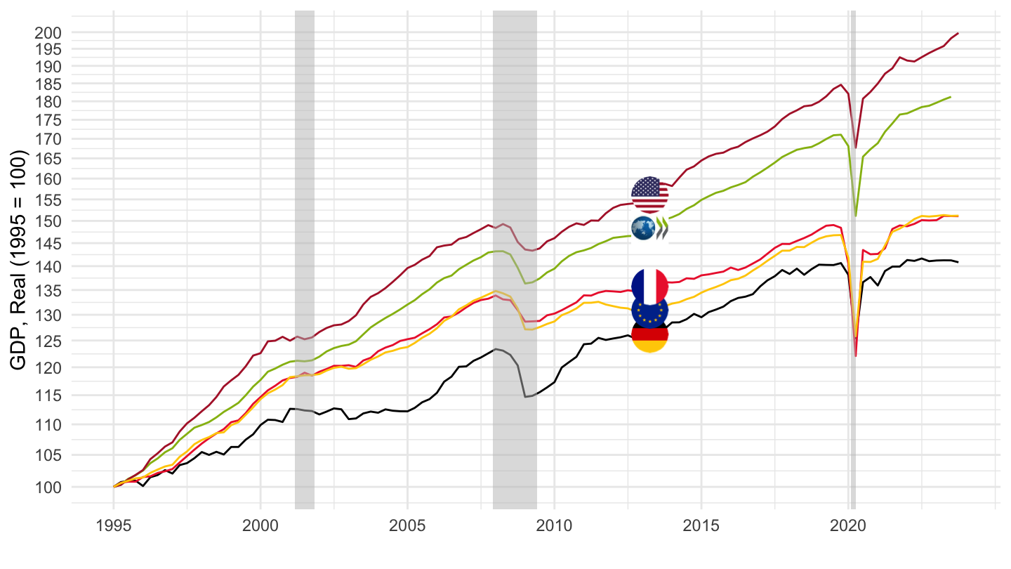

GDP Per Capita

France, Germany, Italy, Spain, United States

1992-

QNA %>%
  filter(LOCATION %in% c("FRA", "DEU", "ITA", "ESP", "USA"),
         SUBJECT == "B1_GE",
         MEASURE == "VOBARSA",
         FREQUENCY == "Q") %>%
  quarter_to_date %>%
  select(LOCATION, date, B1_GE_VOBARSA = obsValue) %>%
  left_join(SNA_TABLE3 %>%
              filter(TRANSACT == "POPNC",
                     MEASURE == "PER") %>%
              year_to_date %>%
              select(LOCATION, date, POPNC_PER = obsValue), 
            by = c("date", "LOCATION")) %>%
  filter(date >= as.Date("1992-01-01"),
         month(date) %% 3 == 1) %>%
  select(LOCATION, date, B1_GE_VOBARSA, POPNC_PER) %>%
  group_by(LOCATION) %>%
  mutate(POPNC_PER_i = spline(x = date, y = POPNC_PER, xout = date)$y,
         obsValue = B1_GE_VOBARSA/POPNC_PER_i) %>%
  left_join(QNA_var$LOCATION, by = "LOCATION") %>%
  mutate(Location = ifelse(LOCATION == "EA20", "Europe", Location)) %>%
  arrange(date) %>%
  mutate(obsValue = 100 * obsValue / obsValue[date == as.Date("1992-01-01")]) %>%
  left_join(colors, by = c("Location" = "country")) %>%
  mutate(color = ifelse(LOCATION == "USA", color2, color)) %>%
  ggplot(.) + theme_minimal() + xlab("") + ylab("GDP Per Capita (1992 = 100)") +
  geom_line(aes(x = date, y = obsValue, color = color)) +
  scale_color_identity() + add_5flags +
  geom_rect(data = nber_recessions %>%
              filter(Peak >= as.Date("1995-01-01")), 
            aes(xmin = Peak, xmax = Trough, ymin = 0, ymax = +Inf), 
            fill = 'grey', alpha = 0.5) +
  scale_x_date(breaks = seq(1960,2100,  2) %>% paste0("-01-01") %>% as.Date,
               labels = date_format("%Y")) +
  scale_y_log10(breaks = seq(70, 200, 5))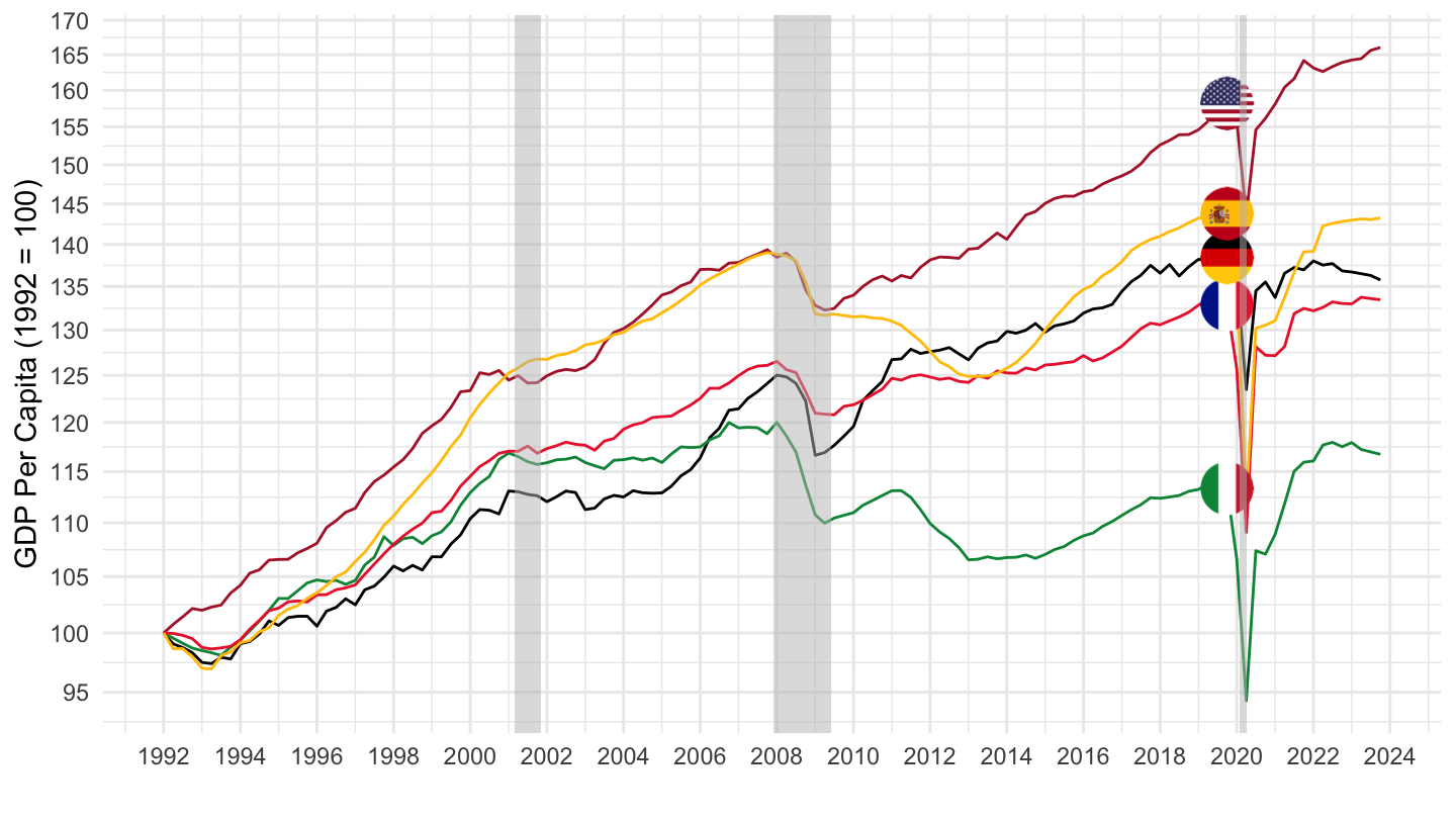

1996-

QNA %>%
  filter(LOCATION %in% c("FRA", "DEU", "ITA", "ESP", "USA"),
         SUBJECT == "B1_GE",
         MEASURE == "VOBARSA",
         FREQUENCY == "Q") %>%
  quarter_to_date %>%
  select(LOCATION, date, B1_GE_VOBARSA = obsValue) %>%
  left_join(SNA_TABLE3 %>%
              filter(TRANSACT == "POPNC",
                     MEASURE == "PER") %>%
              year_to_date %>%
              select(LOCATION, date, POPNC_PER = obsValue), 
            by = c("date", "LOCATION")) %>%
  filter(date >= as.Date("1996-01-01"),
         month(date) %% 3 == 1) %>%
  select(LOCATION, date, B1_GE_VOBARSA, POPNC_PER) %>%
  group_by(LOCATION) %>%
  mutate(POPNC_PER_i = spline(x = date, y = POPNC_PER, xout = date)$y,
         obsValue = B1_GE_VOBARSA/POPNC_PER_i) %>%
  left_join(QNA_var$LOCATION, by = "LOCATION") %>%
  mutate(Location = ifelse(LOCATION == "EA20", "Europe", Location)) %>%
  arrange(date) %>%
  mutate(obsValue = 100 * obsValue / obsValue[date == as.Date("1996-01-01")]) %>%
  left_join(colors, by = c("Location" = "country")) %>%
  mutate(color = ifelse(LOCATION == "USA", color2, color)) %>%
  ggplot(.) + theme_minimal() + xlab("") + ylab("GDP Per Capita, Real (1996 = 100)") +
  geom_line(aes(x = date, y = obsValue, color = color)) +
  scale_color_identity() + add_5flags +
  geom_rect(data = nber_recessions %>%
              filter(Peak >= as.Date("1995-01-01")), 
            aes(xmin = Peak, xmax = Trough, ymin = 0, ymax = +Inf), 
            fill = 'grey', alpha = 0.5) +
  scale_x_date(breaks = seq(1960,2100,  2) %>% paste0("-01-01") %>% as.Date,
               labels = date_format("%Y")) +
  scale_y_log10(breaks = seq(70, 200, 5))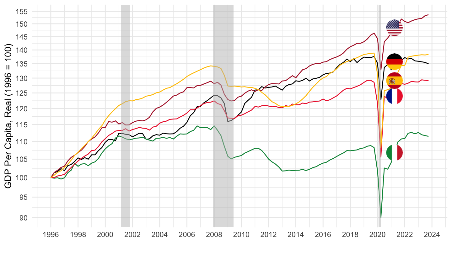

2007-

QNA %>%
  filter(LOCATION %in% c("FRA", "DEU", "ITA", "ESP", "USA"),
         SUBJECT == "B1_GE",
         MEASURE == "VOBARSA",
         FREQUENCY == "Q") %>%
  quarter_to_date %>%
  select(LOCATION, date, B1_GE_VOBARSA = obsValue) %>%
  left_join(SNA_TABLE3 %>%
              filter(TRANSACT == "POPNC",
                     MEASURE == "PER") %>%
              year_to_date %>%
              select(LOCATION, date, POPNC_PER = obsValue), 
            by = c("date", "LOCATION")) %>%
  filter(date >= as.Date("2007-01-01"),
         month(date) %% 3 == 1) %>%
  select(LOCATION, date, B1_GE_VOBARSA, POPNC_PER) %>%
  group_by(LOCATION) %>%
  mutate(POPNC_PER_i = spline(x = date, y = POPNC_PER, xout = date)$y,
         obsValue = B1_GE_VOBARSA/POPNC_PER_i) %>%
  left_join(QNA_var$LOCATION, by = "LOCATION") %>%
  mutate(Location = ifelse(LOCATION == "EA20", "Europe", Location)) %>%
  arrange(date) %>%
  mutate(obsValue = 100 * obsValue / obsValue[date == as.Date("2007-01-01")]) %>%
  left_join(colors, by = c("Location" = "country")) %>%
  mutate(color = ifelse(LOCATION == "USA", color2, color)) %>%
  ggplot(.) + theme_minimal() + xlab("") + ylab("GDP Per Capita (2007 = 100)") +
  geom_line(aes(x = date, y = obsValue, color = color)) +
  scale_color_identity() + add_5flags +
  geom_rect(data = nber_recessions %>%
              filter(Peak >= as.Date("2007-01-01")), 
            aes(xmin = Peak, xmax = Trough, ymin = 0, ymax = +Inf), 
            fill = 'grey', alpha = 0.5) +
  scale_x_date(breaks = seq(1960,2100,  2) %>% paste0("-01-01") %>% as.Date,
               labels = date_format("%Y")) +
  scale_y_log10(breaks = seq(70, 200, 5))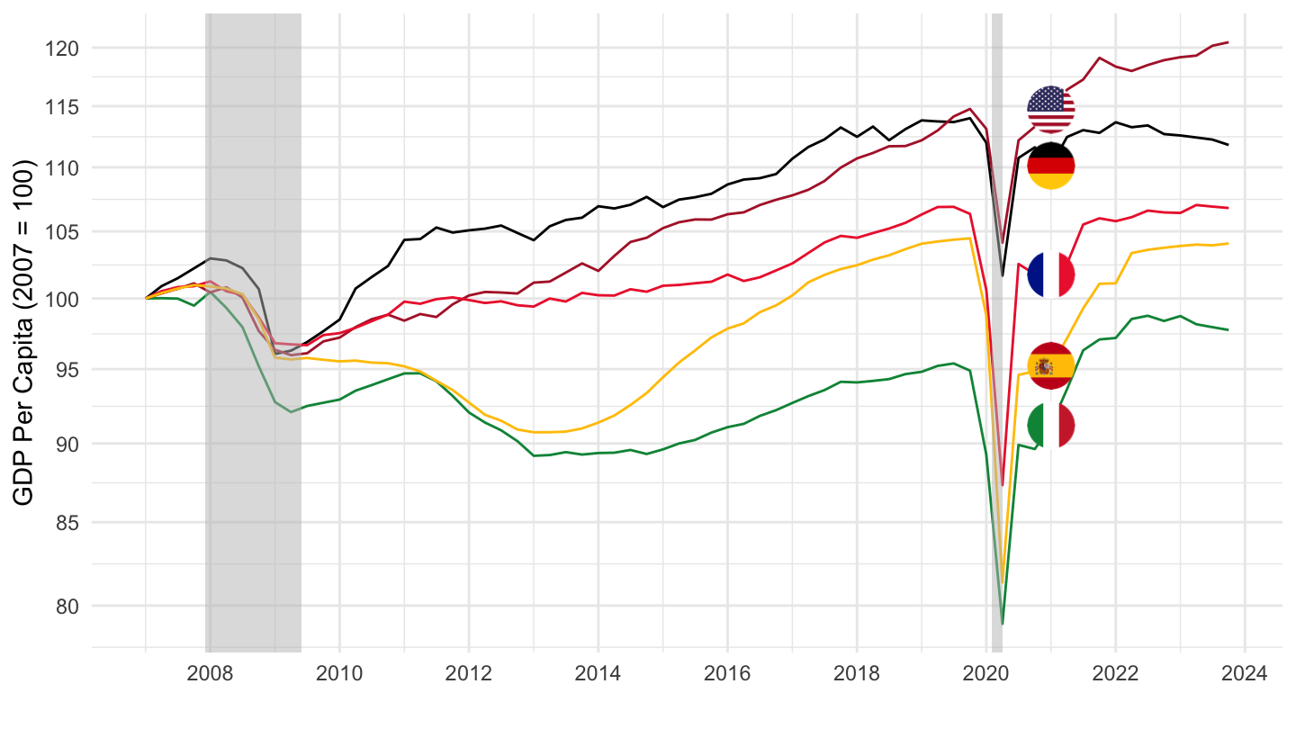

France, Germany, Italy, Spain, Netherlands

1992-

QNA %>%
  filter(LOCATION %in% c("FRA", "DEU", "ITA", "ESP", "NLD"),
         SUBJECT == "B1_GE",
         MEASURE == "VOBARSA",
         FREQUENCY == "Q") %>%
  quarter_to_date %>%
  select(LOCATION, date, B1_GE_VOBARSA = obsValue) %>%
  left_join(SNA_TABLE3 %>%
              filter(TRANSACT == "POPNC",
                     MEASURE == "PER") %>%
              year_to_date %>%
              select(LOCATION, date, POPNC_PER = obsValue), 
            by = c("date", "LOCATION")) %>%
  filter(date >= as.Date("1992-01-01"),
         month(date) %% 3 == 1) %>%
  select(LOCATION, date, B1_GE_VOBARSA, POPNC_PER) %>%
  group_by(LOCATION) %>%
  mutate(POPNC_PER_i = spline(x = date, y = POPNC_PER, xout = date)$y,
         obsValue = B1_GE_VOBARSA/POPNC_PER_i) %>%
  left_join(QNA_var$LOCATION, by = "LOCATION") %>%
  mutate(Location = ifelse(LOCATION == "EA20", "Europe", Location)) %>%
  arrange(date) %>%
  mutate(obsValue = 100 * obsValue / obsValue[date == as.Date("1992-01-01")]) %>%
  left_join(colors, by = c("Location" = "country")) %>%
  mutate(color = ifelse(LOCATION == "NLD", color2, color)) %>%
  ggplot(.) + theme_minimal() + xlab("") + ylab("GDP Per Capita (1992 = 100)") +
  geom_line(aes(x = date, y = obsValue, color = color)) +
  scale_color_identity() + add_5flags +
  geom_rect(data = nber_recessions %>%
              filter(Peak >= as.Date("1995-01-01")), 
            aes(xmin = Peak, xmax = Trough, ymin = 0, ymax = +Inf), 
            fill = 'grey', alpha = 0.5) +
  scale_x_date(breaks = seq(1960,2100,  2) %>% paste0("-01-01") %>% as.Date,
               labels = date_format("%Y")) +
  scale_y_log10(breaks = seq(70, 200, 5))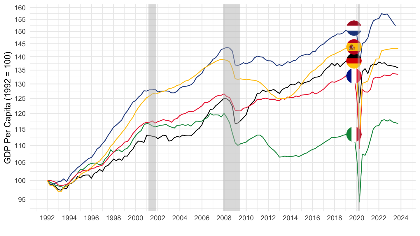

1996-

QNA %>%
  filter(LOCATION %in% c("FRA", "DEU", "ITA", "ESP", "NLD"),
         SUBJECT == "B1_GE",
         MEASURE == "VOBARSA",
         FREQUENCY == "Q") %>%
  quarter_to_date %>%
  select(LOCATION, date, B1_GE_VOBARSA = obsValue) %>%
  left_join(SNA_TABLE3 %>%
              filter(TRANSACT == "POPNC",
                     MEASURE == "PER") %>%
              year_to_date %>%
              select(LOCATION, date, POPNC_PER = obsValue), 
            by = c("date", "LOCATION")) %>%
  filter(date >= as.Date("1996-01-01"),
         month(date) %% 3 == 1) %>%
  select(LOCATION, date, B1_GE_VOBARSA, POPNC_PER) %>%
  group_by(LOCATION) %>%
  mutate(POPNC_PER_i = spline(x = date, y = POPNC_PER, xout = date)$y,
         obsValue = B1_GE_VOBARSA/POPNC_PER_i) %>%
  left_join(QNA_var$LOCATION, by = "LOCATION") %>%
  mutate(Location = ifelse(LOCATION == "EA20", "Europe", Location)) %>%
  arrange(date) %>%
  mutate(obsValue = 100 * obsValue / obsValue[date == as.Date("1996-01-01")]) %>%
  left_join(colors, by = c("Location" = "country")) %>%
  mutate(color = ifelse(LOCATION == "NLD", color2, color)) %>%
  ggplot(.) + theme_minimal() + xlab("") + ylab("GDP Per Capita (1996 = 100)") +
  geom_line(aes(x = date, y = obsValue, color = color)) +
  scale_color_identity() + add_5flags +
  geom_rect(data = nber_recessions %>%
              filter(Peak >= as.Date("1995-01-01")), 
            aes(xmin = Peak, xmax = Trough, ymin = 0, ymax = +Inf), 
            fill = 'grey', alpha = 0.5) +
  scale_x_date(breaks = seq(1960,2100,  2) %>% paste0("-01-01") %>% as.Date,
               labels = date_format("%Y")) +
  scale_y_log10(breaks = seq(70, 200, 5))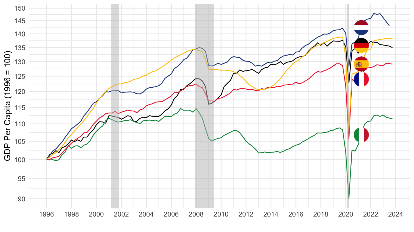

US, Europe, France, Germany

1990-

QNA %>%
  filter(LOCATION %in% c("USA", "EA20", "FRA", "DEU"),
         SUBJECT == "B1_GE",
         MEASURE == "VOBARSA",
         FREQUENCY == "Q") %>%
  quarter_to_date %>%
  select(LOCATION, date, B1_GE_VOBARSA = obsValue) %>%
  left_join(SNA_TABLE3 %>%
              filter(TRANSACT == "POPNC",
                     MEASURE == "PER") %>%
              year_to_date %>%
              select(LOCATION, date, POPNC_PER = obsValue), 
            by = c("date", "LOCATION")) %>%
  filter(date >= as.Date("1989-10-01"),
         month(date) %% 3 == 1) %>%
  mutate(date = date + months(3) -days(1)) %>%
  select(LOCATION, date, B1_GE_VOBARSA, POPNC_PER) %>%
  group_by(LOCATION) %>%
  mutate(POPNC_PER_i = spline(x = date, y = POPNC_PER, xout = date)$y,
         obsValue = B1_GE_VOBARSA/POPNC_PER_i) %>%
  left_join(QNA_var$LOCATION, by = "LOCATION") %>%
  mutate(Location = ifelse(LOCATION == "EA20", "Europe", Location)) %>%
  arrange(date) %>%
  mutate(obsValue = 100 * obsValue / obsValue[date == as.Date("2007-06-30")]) %>%
  left_join(colors, by = c("Location" = "country")) %>%
  mutate(color = ifelse(LOCATION == "USA", color2, color),
         color = ifelse(LOCATION == "EA20", color2, color)) %>%
  ggplot(.) + theme_minimal() + xlab("") + ylab("GDP Per Capita (2007 = 100)") +
  geom_line(aes(x = date, y = obsValue, color = color)) +
  scale_color_identity() + add_4flags +
  geom_rect(data = nber_recessions %>%
              filter(Peak >= as.Date("1995-01-01")), 
            aes(xmin = Peak, xmax = Trough, ymin = 0, ymax = +Inf), 
            fill = 'grey', alpha = 0.5) +
  scale_x_date(breaks = seq(1960,2100,  2) %>% paste0("-01-01") %>% as.Date,
               labels = date_format("%Y")) +
  scale_y_log10(breaks = seq(70, 200, 2))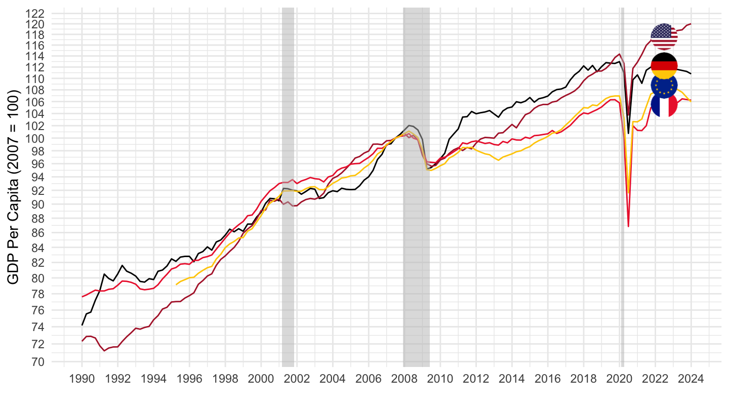

1995-

Base 100

QNA %>%
  filter(LOCATION %in% c("USA", "EA20", "FRA", "DEU"),
         SUBJECT == "B1_GE",
         MEASURE == "VOBARSA",
         FREQUENCY == "Q") %>%
  quarter_to_date %>%
  select(LOCATION, date, B1_GE_VOBARSA = obsValue) %>%
  left_join(SNA_TABLE3 %>%
              filter(TRANSACT == "POPNC",
                     MEASURE == "PER") %>%
              year_to_date %>%
              select(LOCATION, date, POPNC_PER = obsValue), 
            by = c("date", "LOCATION")) %>%
  filter(date >= as.Date("1995-01-01"),
         month(date) %% 3 == 1) %>%
  select(LOCATION, date, B1_GE_VOBARSA, POPNC_PER) %>%
  group_by(LOCATION) %>%
  mutate(POPNC_PER_i = spline(x = date, y = POPNC_PER, xout = date)$y,
         obsValue = B1_GE_VOBARSA/POPNC_PER_i) %>%
  left_join(QNA_var$LOCATION, by = "LOCATION") %>%
  mutate(Location = ifelse(LOCATION == "EA20", "Europe", Location)) %>%
  arrange(date) %>%
  mutate(obsValue = 100 * obsValue / obsValue[date == as.Date("1995-01-01")]) %>%
  left_join(colors, by = c("Location" = "country")) %>%
  mutate(color = ifelse(LOCATION == "USA", color2, color),
         color = ifelse(LOCATION == "EA20", color2, color)) %>%
  ggplot(.) + theme_minimal() + xlab("") + ylab("GDP Per Capita (1995 = 100)") +
  geom_line(aes(x = date, y = obsValue, color = color)) +
  scale_color_identity() + add_4flags +
  geom_rect(data = nber_recessions %>%
              filter(Peak >= as.Date("1995-01-01")), 
            aes(xmin = Peak, xmax = Trough, ymin = 0, ymax = +Inf), 
            fill = 'grey', alpha = 0.5) +
  scale_x_date(breaks = seq(1960, 2022, 5) %>% paste0("-01-01") %>% as.Date,
               labels = date_format("%Y")) +
  scale_y_log10(breaks = seq(70, 200, 5))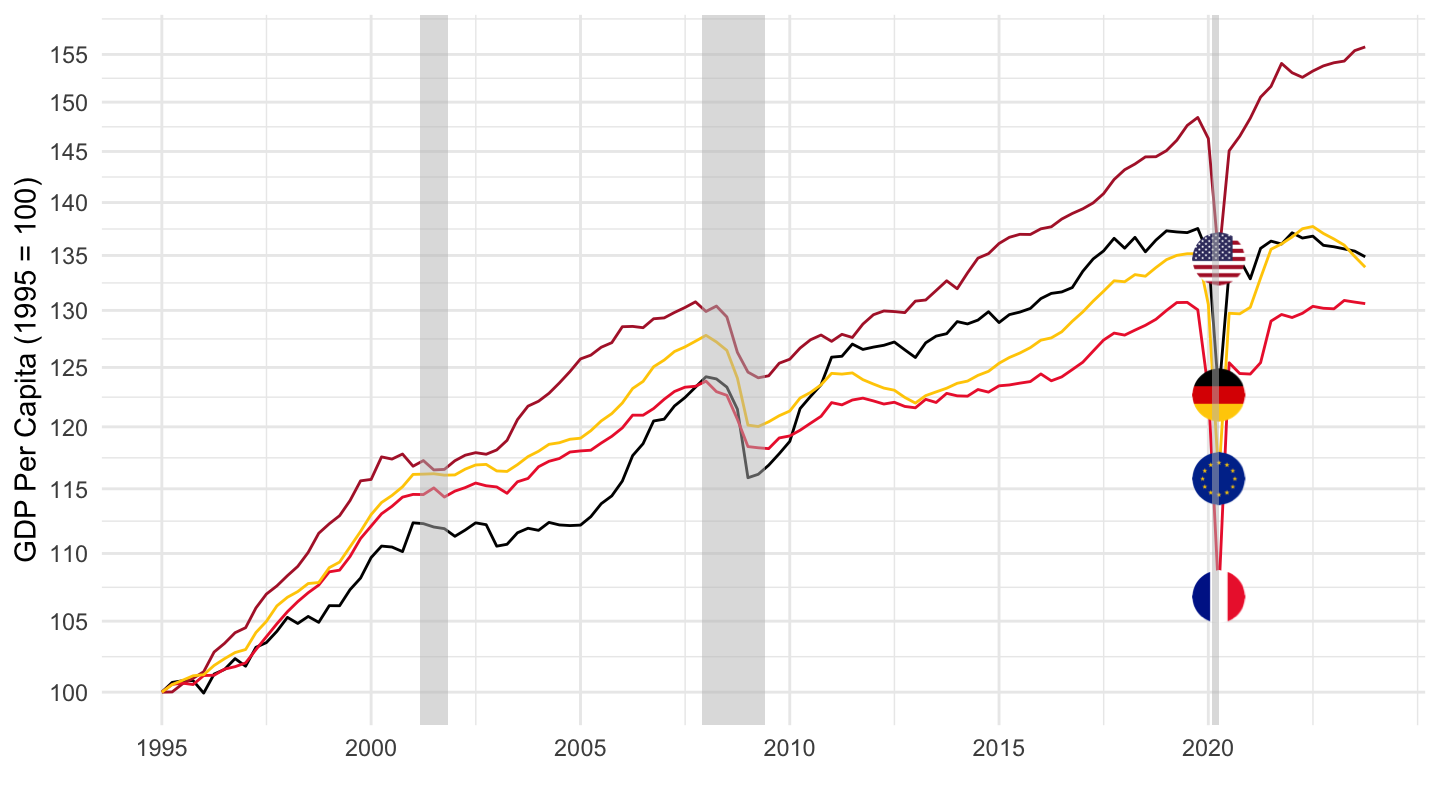

Dollars

QNA %>%
  filter(LOCATION %in% c("USA", "EA20", "FRA", "DEU", "ITA"),
         SUBJECT == "B1_GE",
         MEASURE == "VOBARSA",
         FREQUENCY == "Q") %>%
  quarter_to_date %>%
  select(LOCATION, date, B1_GE_VOBARSA = obsValue) %>%
  left_join(SNA_TABLE3 %>%
              filter(TRANSACT == "POPNC",
                     MEASURE == "PER") %>%
              year_to_date %>%
              select(LOCATION, date, POPNC_PER = obsValue), 
            by = c("date", "LOCATION")) %>%
  filter(date >= as.Date("1995-01-01"),
         month(date) %% 3 == 1) %>%
  select(LOCATION, date, B1_GE_VOBARSA, POPNC_PER) %>%
  group_by(LOCATION) %>%
  mutate(POPNC_PER_i = spline(x = date, y = POPNC_PER, xout = date)$y,
         obsValue = 1000*B1_GE_VOBARSA/POPNC_PER_i) %>%
  left_join(QNA_var$LOCATION, by = "LOCATION") %>%
  mutate(Location = ifelse(LOCATION == "EA20", "Europe", Location)) %>%
  arrange(date) %>%
  left_join(colors, by = c("Location" = "country")) %>%
  mutate(color = ifelse(LOCATION == "USA", color2, color),
         color = ifelse(LOCATION == "EA20", color2, color)) %>%
  ggplot(.) + theme_minimal() + xlab("") + ylab("PIB Par Habitant ($)") +
  geom_line(aes(x = date, y = obsValue, color = color)) +
  scale_color_identity() + add_5flags +
  geom_rect(data = nber_recessions %>%
              filter(Peak >= as.Date("1995-01-01")), 
            aes(xmin = Peak, xmax = Trough, ymin = 0, ymax = +Inf), 
            fill = 'grey', alpha = 0.5) +
  scale_x_date(breaks = seq(1960, 2022, 5) %>% paste0("-01-01") %>% as.Date,
               labels = date_format("%Y")) +
  scale_y_log10(breaks = seq(10000, 200000, 5000),
                labels = dollar_format(acc = 1))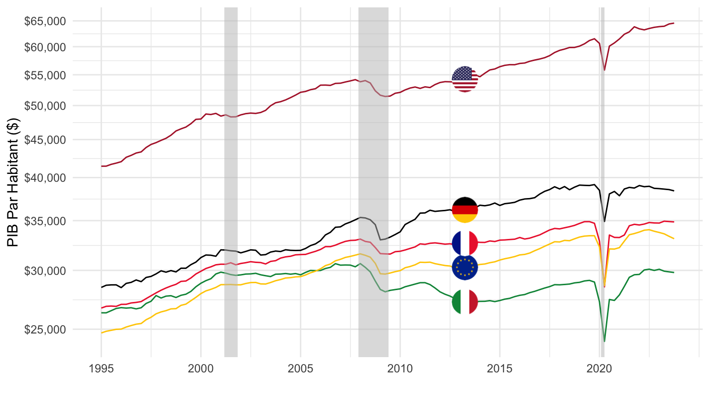

Dollars PPP

QNA %>%
  filter(LOCATION %in% c("USA", "EA20", "FRA", "DEU", "ITA"),
         SUBJECT == "B1_GE",
         MEASURE == "VPVOBARSA",
         FREQUENCY == "Q") %>%
  quarter_to_date %>%
  select(LOCATION, date, B1_GE_VOBARSA = obsValue) %>%
  left_join(SNA_TABLE3 %>%
              filter(TRANSACT == "POPNC",
                     MEASURE == "PER") %>%
              year_to_date %>%
              select(LOCATION, date, POPNC_PER = obsValue), 
            by = c("date", "LOCATION")) %>%
  filter(date >= as.Date("1995-01-01"),
         month(date) %% 3 == 1) %>%
  select(LOCATION, date, B1_GE_VOBARSA, POPNC_PER) %>%
  group_by(LOCATION) %>%
  mutate(POPNC_PER_i = spline(x = date, y = POPNC_PER, xout = date)$y,
         obsValue = 1000*B1_GE_VOBARSA/POPNC_PER_i) %>%
  left_join(QNA_var$LOCATION, by = "LOCATION") %>%
  mutate(Location = ifelse(LOCATION == "EA20", "Europe", Location)) %>%
  arrange(date) %>%
  left_join(colors, by = c("Location" = "country")) %>%
  mutate(color = ifelse(LOCATION == "USA", color2, color),
         color = ifelse(LOCATION == "EA20", color2, color)) %>%
  ggplot(.) + theme_minimal() + xlab("") + ylab("PIB Par Habitant ($ PPP 2015)") +
  geom_line(aes(x = date, y = obsValue, color = color)) +
  scale_color_identity() + add_5flags +
  geom_rect(data = nber_recessions %>%
              filter(Peak >= as.Date("1995-01-01")), 
            aes(xmin = Peak, xmax = Trough, ymin = 0, ymax = +Inf), 
            fill = 'grey', alpha = 0.5) +
  scale_x_date(breaks = seq(1960, 2022, 5) %>% paste0("-01-01") %>% as.Date,
               labels = date_format("%Y")) +
  scale_y_log10(breaks = seq(10000, 200000, 5000),
                labels = dollar_format(acc = 1))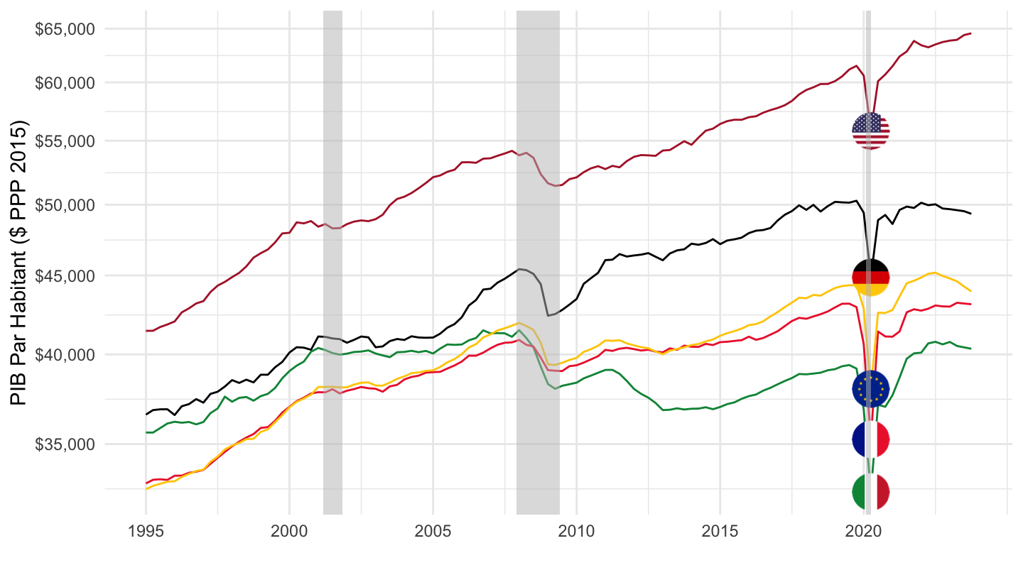

PPP Dollars

QNA %>%
  filter(LOCATION %in% c("USA", "EA20", "FRA", "DEU"),
         SUBJECT == "B1_GE",
         MEASURE == "VPVOBARSA",
         FREQUENCY == "Q") %>%
  quarter_to_date %>%
  select(LOCATION, date, B1_GE_VOBARSA = obsValue) %>%
  left_join(SNA_TABLE3 %>%
              filter(TRANSACT == "POPNC",
                     MEASURE == "PER") %>%
              year_to_date %>%
              select(LOCATION, date, POPNC_PER = obsValue), 
            by = c("date", "LOCATION")) %>%
  filter(date >= as.Date("1995-01-01"),
         month(date) %% 3 == 1) %>%
  select(LOCATION, date, B1_GE_VOBARSA, POPNC_PER) %>%
  group_by(LOCATION) %>%
  mutate(POPNC_PER_i = spline(x = date, y = POPNC_PER, xout = date)$y,
         obsValue = 1000*B1_GE_VOBARSA/POPNC_PER_i) %>%
  left_join(QNA_var$LOCATION, by = "LOCATION") %>%
  mutate(Location = ifelse(LOCATION == "EA20", "Europe", Location)) %>%
  arrange(date) %>%
  left_join(colors, by = c("Location" = "country")) %>%
  mutate(color = ifelse(LOCATION == "USA", color2, color),
         color = ifelse(LOCATION == "EA20", color2, color)) %>%
  ggplot(.) + theme_minimal() + xlab("") + ylab("PIB Par Habitant ($ PPP)") +
  geom_line(aes(x = date, y = obsValue, color = color)) +
  scale_color_identity() + add_4flags +
  geom_rect(data = nber_recessions %>%
              filter(Peak >= as.Date("1995-01-01")), 
            aes(xmin = Peak, xmax = Trough, ymin = 0, ymax = +Inf), 
            fill = 'grey', alpha = 0.5) +
  scale_x_date(breaks = seq(1960, 2022, 5) %>% paste0("-01-01") %>% as.Date,
               labels = date_format("%Y")) +
  scale_y_log10(breaks = seq(10000, 200000, 5000),
                labels = dollar_format(acc = 1))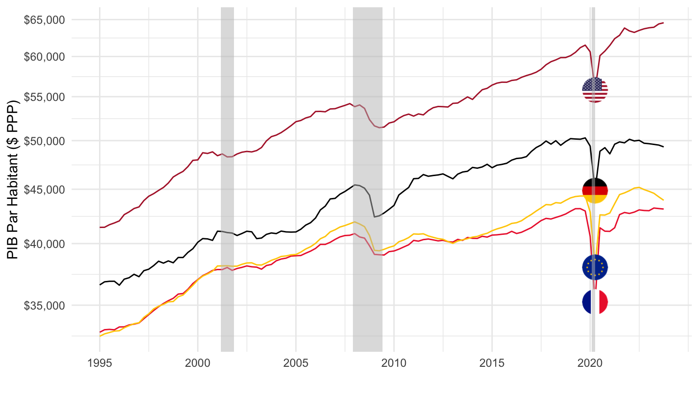

Par travailleur: ETO

QNA %>%
  filter(LOCATION %in% c("USA", "EA20", "FRA", "DEU"),
         SUBJECT == "B1_GE",
         MEASURE == "VPVOBARSA",
         FREQUENCY == "Q") %>%
  quarter_to_date %>%
  select(LOCATION, date, B1_GE_VOBARSA = obsValue) %>%
  left_join(SNA_TABLE3 %>%
              filter(TRANSACT == "ETO",
                     MEASURE == "PER") %>%
              year_to_date %>%
              select(LOCATION, date, POPNC_PER = obsValue), 
            by = c("date", "LOCATION")) %>%
  filter(date >= as.Date("1995-01-01"),
         month(date) %% 3 == 1,
         date <= as.Date("2020-01-01")) %>%
  select(LOCATION, date, B1_GE_VOBARSA, POPNC_PER) %>%
  group_by(LOCATION) %>%
  mutate(POPNC_PER_i = spline(x = date, y = POPNC_PER, xout = date)$y,
         obsValue = 1000*B1_GE_VOBARSA/POPNC_PER_i) %>%
  left_join(QNA_var$LOCATION, by = "LOCATION") %>%
  mutate(Location = ifelse(LOCATION == "EA20", "Europe", Location)) %>%
  arrange(date) %>%
  left_join(colors, by = c("Location" = "country")) %>%
  mutate(color = ifelse(LOCATION == "USA", color2, color),
         color = ifelse(LOCATION == "EA20", color2, color)) %>%
  ggplot(.) + theme_minimal() + xlab("") + ylab("PIB Par Habitant ($ PPP)") +
  geom_line(aes(x = date, y = obsValue, color = color)) +
  scale_color_identity() + add_4flags +
  geom_rect(data = nber_recessions %>%
              filter(Peak >= as.Date("1995-01-01")), 
            aes(xmin = Peak, xmax = Trough, ymin = 0, ymax = +Inf), 
            fill = 'grey', alpha = 0.5) +
  scale_x_date(breaks = seq(1960, 2022, 5) %>% paste0("-01-01") %>% as.Date,
               labels = date_format("%Y")) +
  scale_y_log10(breaks = seq(10000, 200000, 5000),
                labels = dollar_format(acc = 1))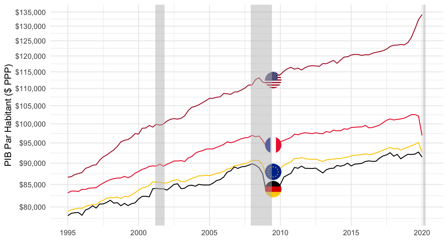

1996-

QNA %>%
  filter(LOCATION %in% c("USA", "EA20", "FRA", "DEU", "ITA"),
         SUBJECT == "B1_GE",
         MEASURE == "VOBARSA",
         FREQUENCY == "Q") %>%
  quarter_to_date %>%
  select(LOCATION, date, B1_GE_VOBARSA = obsValue) %>%
  left_join(SNA_TABLE3 %>%
              filter(TRANSACT == "POPNC",
                     MEASURE == "PER") %>%
              year_to_date %>%
              select(LOCATION, date, POPNC_PER = obsValue), 
            by = c("date", "LOCATION")) %>%
  filter(date >= as.Date("1996-01-01"),
         month(date) %% 3 == 1) %>%
  select(LOCATION, date, B1_GE_VOBARSA, POPNC_PER) %>%
  group_by(LOCATION) %>%
  mutate(POPNC_PER_i = spline(x = date, y = POPNC_PER, xout = date)$y,
         obsValue = B1_GE_VOBARSA/POPNC_PER_i) %>%
  left_join(QNA_var$LOCATION, by = "LOCATION") %>%
  mutate(Location = ifelse(LOCATION == "EA20", "Europe", Location)) %>%
  arrange(date) %>%
  mutate(obsValue = 100 * obsValue / obsValue[date == as.Date("1996-01-01")]) %>%
  left_join(colors, by = c("Location" = "country")) %>%
  mutate(color = ifelse(LOCATION == "USA", color2, color),
         color = ifelse(LOCATION == "EA20", color2, color)) %>%
  ggplot(.) + theme_minimal() + xlab("") + ylab("GDP Per Capita (1996 = 100)") +
  geom_line(aes(x = date, y = obsValue, color = color)) +
  scale_color_identity() + add_5flags +
  geom_rect(data = nber_recessions %>%
              filter(Peak >= as.Date("1995-01-01")), 
            aes(xmin = Peak, xmax = Trough, ymin = 0, ymax = +Inf), 
            fill = 'grey', alpha = 0.5) +
  scale_x_date(breaks = seq(1960,2100,  2) %>% paste0("-01-01") %>% as.Date,
               labels = date_format("%Y")) +
  scale_y_log10(breaks = seq(70, 200, 5))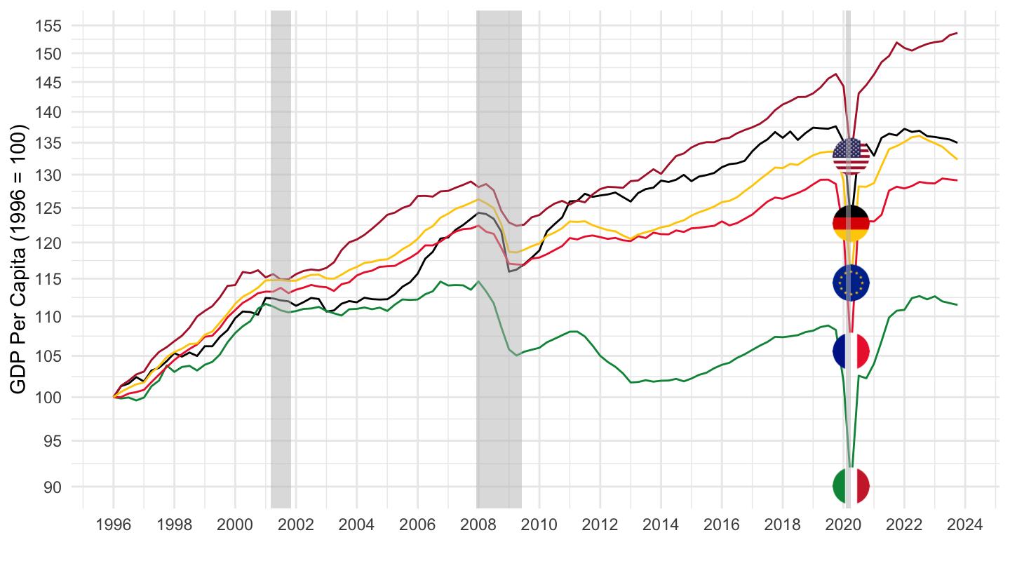

2000-

QNA %>%
  filter(LOCATION %in% c("USA", "EA20", "FRA", "DEU"),
         SUBJECT == "B1_GE",
         MEASURE == "VOBARSA",
         FREQUENCY == "Q") %>%
  quarter_to_date %>%
  select(LOCATION, date, B1_GE_VOBARSA = obsValue) %>%
  left_join(SNA_TABLE3 %>%
              filter(TRANSACT == "POPNC",
                     MEASURE == "PER") %>%
              year_to_date %>%
              select(LOCATION, date, POPNC_PER = obsValue), 
            by = c("date", "LOCATION")) %>%
  filter(date >= as.Date("1999-10-01"),
         month(date) %% 3 == 1) %>%
  mutate(date = date + months(3) -days(1)) %>%
  select(LOCATION, date, B1_GE_VOBARSA, POPNC_PER) %>%
  group_by(LOCATION) %>%
  mutate(POPNC_PER_i = spline(x = date, y = POPNC_PER, xout = date)$y,
         obsValue = B1_GE_VOBARSA/POPNC_PER_i) %>%
  left_join(QNA_var$LOCATION, by = "LOCATION") %>%
  mutate(Location = ifelse(LOCATION == "EA20", "Europe", Location)) %>%
  arrange(date) %>%
  mutate(obsValue = 100 * obsValue / obsValue[date == as.Date("2007-06-30")]) %>%
  left_join(colors, by = c("Location" = "country")) %>%
  mutate(color = ifelse(LOCATION == "USA", color2, color),
         color = ifelse(LOCATION == "EA20", color2, color)) %>%
  ggplot(.) + theme_minimal() + xlab("") + ylab("GDP Per Capita (2007 = 100)") +
  geom_line(aes(x = date, y = obsValue, color = color)) +
  scale_color_identity() + add_4flags +
  geom_rect(data = nber_recessions %>%
              filter(Peak >= as.Date("1995-01-01")), 
            aes(xmin = Peak, xmax = Trough, ymin = 0, ymax = +Inf), 
            fill = 'grey', alpha = 0.5) +
  scale_x_date(breaks = seq(1960,2100,  2) %>% paste0("-01-01") %>% as.Date,
               labels = date_format("%Y")) +
  scale_y_log10(breaks = seq(70, 200, 2))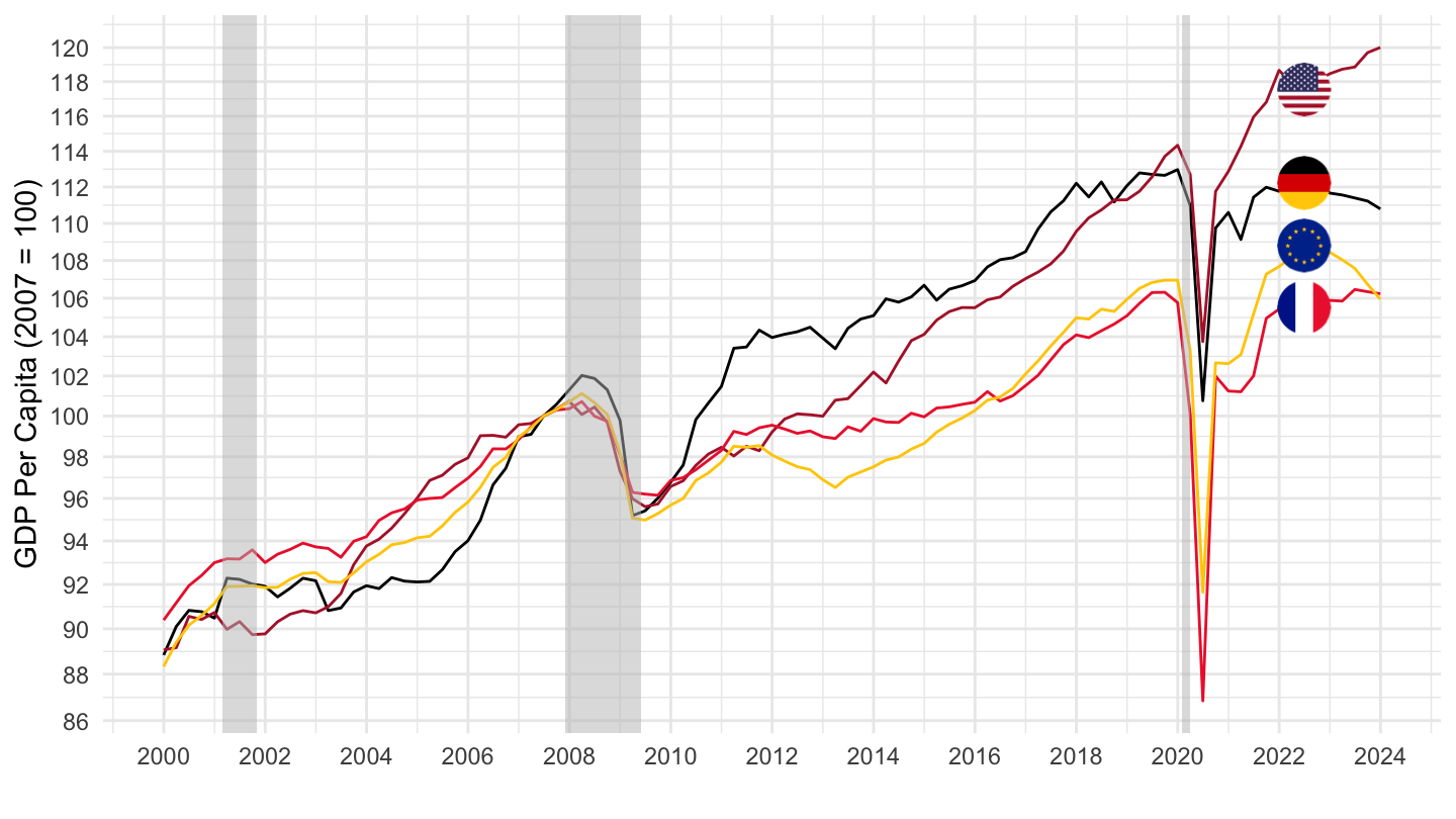

US, Europe, France, Germany, Italy

QNA %>%
  filter(LOCATION %in% c("USA", "EA20", "FRA", "DEU", "ITA"),
         SUBJECT == "B1_GE",
         MEASURE == "VOBARSA",
         FREQUENCY == "Q") %>%
  quarter_to_date %>%
  select(LOCATION, date, B1_GE_VOBARSA = obsValue) %>%
  left_join(SNA_TABLE3 %>%
              filter(TRANSACT == "POPNC",
                     MEASURE == "PER") %>%
              year_to_date %>%
              select(LOCATION, date, POPNC_PER = obsValue), 
            by = c("date", "LOCATION")) %>%
  filter(date >= as.Date("1999-10-01"),
         month(date) %% 3 == 1) %>%
  mutate(date = date + months(3) -days(1)) %>%
  select(LOCATION, date, B1_GE_VOBARSA, POPNC_PER) %>%
  group_by(LOCATION) %>%
  mutate(POPNC_PER_i = spline(x = date, y = POPNC_PER, xout = date)$y,
         obsValue = B1_GE_VOBARSA/POPNC_PER_i) %>%
  left_join(QNA_var$LOCATION, by = "LOCATION") %>%
  mutate(Location = ifelse(LOCATION == "EA20", "Europe", Location)) %>%
  arrange(date) %>%
  mutate(obsValue = 100 * obsValue / obsValue[date == as.Date("2007-06-30")]) %>%
  left_join(colors, by = c("Location" = "country")) %>%
  mutate(color = ifelse(LOCATION == "USA", color2, color),
         color = ifelse(LOCATION == "EA20", color2, color)) %>%
  ggplot(.) + theme_minimal() + xlab("") + ylab("GDP Per Capita (2007 = 100)") +
  geom_line(aes(x = date, y = obsValue, color = color)) +
  scale_color_identity() + add_5flags +
  geom_rect(data = nber_recessions %>%
              filter(Peak >= as.Date("1995-01-01")), 
            aes(xmin = Peak, xmax = Trough, ymin = 0, ymax = +Inf), 
            fill = 'grey', alpha = 0.5) +
  scale_x_date(breaks = seq(1960,2100,  2) %>% paste0("-01-01") %>% as.Date,
               labels = date_format("%Y")) +
  scale_y_log10(breaks = seq(70, 200, 2))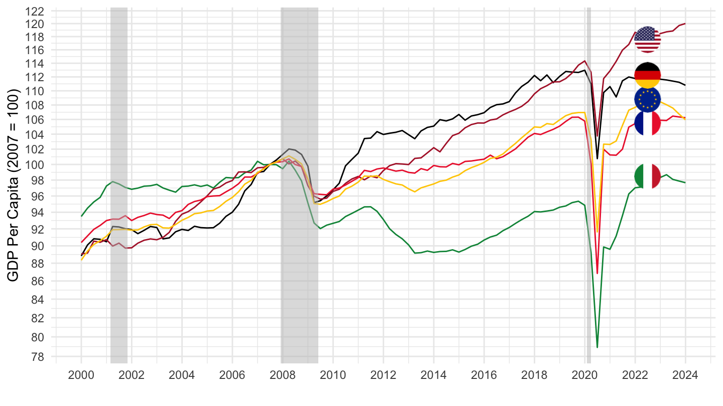

Italy, Spain, France, Germany

QNA %>%
  filter(LOCATION %in% c("ITA", "ESP", "FRA", "DEU", "USA"),
         SUBJECT == "B1_GE",
         MEASURE == "VOBARSA",
         FREQUENCY == "Q") %>%
  quarter_to_date %>%
  select(LOCATION, date, B1_GE_VOBARSA = obsValue) %>%
  left_join(SNA_TABLE3 %>%
              filter(TRANSACT == "POPNC",
                     MEASURE == "PER") %>%
              year_to_date %>%
              select(LOCATION, date, POPNC_PER = obsValue), 
            by = c("date", "LOCATION")) %>%
  filter(date >= as.Date("1999-10-01"),
         month(date) %% 3 == 1) %>%
  mutate(date = date + months(3) -days(1)) %>%
  select(LOCATION, date, B1_GE_VOBARSA, POPNC_PER) %>%
  group_by(LOCATION) %>%
  mutate(POPNC_PER_i = spline(x = date, y = POPNC_PER, xout = date)$y,
         obsValue = B1_GE_VOBARSA/POPNC_PER_i) %>%
  left_join(QNA_var$LOCATION, by = "LOCATION") %>%
  mutate(Location = ifelse(LOCATION == "EA20", "Europe", Location)) %>%
  arrange(date) %>%
  mutate(obsValue = 100 * obsValue / obsValue[date == as.Date("2007-06-30")]) %>%
  left_join(colors, by = c("Location" = "country")) %>%
  mutate(color = ifelse(LOCATION == "USA", color2, color),
         color = ifelse(LOCATION == "EA20", color2, color)) %>%
  ggplot(.) + theme_minimal() + xlab("") + ylab("GDP Per Capita (2007 = 100)") +
  geom_line(aes(x = date, y = obsValue, color = color)) +
  scale_color_identity() + add_5flags +
  geom_rect(data = nber_recessions %>%
              filter(Peak >= as.Date("1995-01-01")), 
            aes(xmin = Peak, xmax = Trough, ymin = 0, ymax = +Inf), 
            fill = 'grey', alpha = 0.5) +
  scale_x_date(breaks = seq(1960,2100,  2) %>% paste0("-01-01") %>% as.Date,
               labels = date_format("%Y")) +
  scale_y_log10(breaks = seq(70, 200, 2))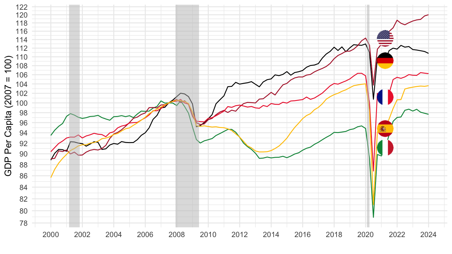

Netherlands, Portugal

QNA %>%
  filter(LOCATION %in% c("NLD", "PRT", "BEL"),
         SUBJECT == "B1_GE",
         MEASURE == "VOBARSA",
         FREQUENCY == "Q") %>%
  quarter_to_date %>%
  select(LOCATION, date, B1_GE_VOBARSA = obsValue) %>%
  left_join(SNA_TABLE3 %>%
              filter(TRANSACT == "POPNC",
                     MEASURE == "PER") %>%
              year_to_date %>%
              select(LOCATION, date, POPNC_PER = obsValue), 
            by = c("date", "LOCATION")) %>%
  filter(date >= as.Date("1999-10-01"),
         month(date) %% 3 == 1) %>%
  mutate(date = date + months(3) -days(1)) %>%
  select(LOCATION, date, B1_GE_VOBARSA, POPNC_PER) %>%
  group_by(LOCATION) %>%
  mutate(POPNC_PER_i = spline(x = date, y = POPNC_PER, xout = date)$y,
         obsValue = B1_GE_VOBARSA/POPNC_PER_i) %>%
  left_join(QNA_var$LOCATION, by = "LOCATION") %>%
  mutate(Location = ifelse(LOCATION == "EA20", "Europe", Location)) %>%
  arrange(date) %>%
  mutate(obsValue = 100 * obsValue / obsValue[date == as.Date("2007-06-30")]) %>%
  left_join(colors, by = c("Location" = "country")) %>%
  mutate(color = ifelse(LOCATION == "USA", color2, color),
         color = ifelse(LOCATION == "EA20", color2, color)) %>%
  ggplot(.) + theme_minimal() + xlab("") + ylab("GDP Per Capita (2007 = 100)") +
  geom_line(aes(x = date, y = obsValue, color = color)) +
  scale_color_identity() + add_3flags +
  geom_rect(data = nber_recessions %>%
              filter(Peak >= as.Date("1995-01-01")), 
            aes(xmin = Peak, xmax = Trough, ymin = 0, ymax = +Inf), 
            fill = 'grey', alpha = 0.5) +
  scale_x_date(breaks = seq(1960,2100,  2) %>% paste0("-01-01") %>% as.Date,
               labels = date_format("%Y")) +
  scale_y_log10(breaks = seq(70, 200, 2))

Quarterly National Accounts - Live

Data - OECD

François Geerolf

Info

Data on macro

Last

Real GDP Last

QNA Live

Last, France

Last, Germany

Horse Races

Greece

Germany, US VS France

2007-

2001- (introduction Euro)

With Italy

Base 2007

Base 2001

French

Eurozone VS Eurone

2000-

English

US VS Europe

2000-

population

English

French

Flags

French

US VS Europe

2000-

English

French (Base = 2007)

All

With ticks

GDP per capita

Consumption per capita

Investment per capita

French (Base = 2014)

2010-

French (Base = 2007)

French (Base = 2014)

1995-

French

1996-

French

2000-

2015-

US, Europe, OECD

Tous

US, Europe, Italy

Tous

1995-

English

French

Europe VS Japan

100 = 2003

100 = 2000

100 = 1995

US VS Europe VS Sweden

Ex 1

France, Italy, Europe, US, Germany

Base 100

1995-

VOBARSA

VOBARSA

GDP

CPCARSA - US dollars, current prices, current PPPs, annual levels, seasonally adjusted

VPVOBARSA - US dollars, volume estimates, fixed PPPs (2015), OECD reference year, annual levels, seasonally adjusted

France, Germany, Italy, Spain, United States

1992-

1996-

EU, France, Germany, US

1995-

EU, France, Germany, US, Japan

1995-

GDP Per Capita

France, Germany, Italy, Spain, United States

1992-

1996-