Population and employment by main activity

Data - OECD

Author

Info

source	dataset	.html	.RData
oecd	SNA_TABLE3	2024-06-19	2024-04-16

Données sur l’industrie

source	dataset	.html	.RData
eurostat	mar_mg_am_cvh	2024-06-20	2024-06-08
eurostat	namq_10_a10	2024-06-20	2024-06-18
insee	CNA-2014-EMPLOI	2024-06-07	2024-06-18
insee	CNT-2014-CB	2024-06-20	2024-06-18
insee	CNT-2014-OPERATIONS	2024-06-20	2024-06-18
insee	ENQ-CONJ-ACT-IND	2024-06-20	2024-06-18
insee	ICA-2015-IND-CONS	2024-06-20	2024-06-18
insee	IPI-2021	2024-06-08	2024-06-06
insee	IPPI-2015	2024-06-20	2024-06-19
insee	t_5407	2024-06-20	2021-08-01
insee	TCRED-EMPLOI-SALARIE-TRIM	2024-06-20	2024-06-19
oecd	ALFS_EMP	2024-04-16	2024-05-12
oecd	SNA_TABLE3	2024-06-19	2024-04-16

LAST_COMPILE

LAST_COMPILE
2024-06-20

Last

obsTime	Nobs
2023	188

Layout

OECD Website. html

TRANSACT

Code

SNA_TABLE3 %>%
  left_join(SNA_TABLE3_var$TRANSACT, by = "TRANSACT") %>%
  group_by(TRANSACT, Transact) %>%
  summarise(Nobs = n()) %>%
  arrange(-Nobs) %>%
  print_table_conditional()

MEASURE

Code

SNA_TABLE3 %>%
  left_join(SNA_TABLE3_var$MEASURE, by = "MEASURE") %>%
  group_by(MEASURE, Measure) %>%
  summarise(Nobs = n()) %>%
  print_table_conditional()

MEASURE	Measure	Nobs
FTE	Full-time equivalents	5544
HRS	Hours	47402
JOB	Jobs	13379
PER	Persons	62019

LOCATION

Code

SNA_TABLE3 %>%
  left_join(SNA_TABLE3_var$LOCATION, by = "LOCATION") %>%
  group_by(LOCATION, Location) %>%
  summarise(Nobs = n()) %>%
  arrange(-Nobs) %>%
  mutate(Flag = gsub(" ", "-", str_to_lower(gsub(" ", "-", Location))),
         Flag = paste0('<img src="../../icon/flag/vsmall/', Flag, '.png" alt="Flag">')) %>%
  select(Flag, everything()) %>%
  {if (is_html_output()) datatable(., filter = 'top', rownames = F, escape = F) else .}

PER - Persons (Thousands)

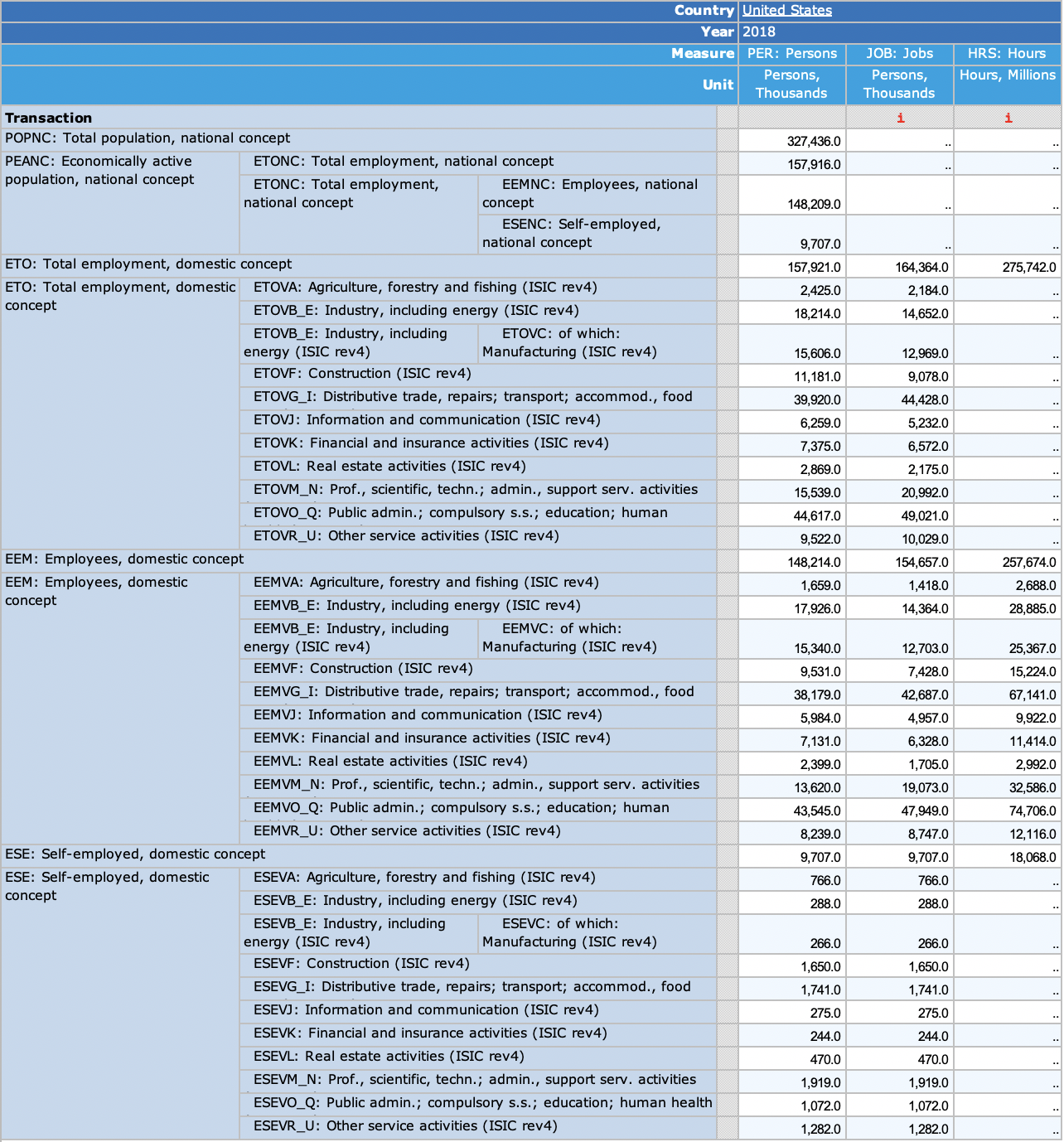
France, Germany, United States

Code

SNA_TABLE3 %>%
  filter(obsTime == "2018",
         LOCATION %in% c("FRA", "DEU", "USA"),
         MEASURE == "PER") %>%
  left_join(SNA_TABLE3_var$TRANSACT, by = "TRANSACT") %>%
  select(LOCATION, TRANSACT, Transact, obsValue) %>%
  mutate(obsValue = round(obsValue)) %>%
  spread(LOCATION, obsValue) %>%
  {if (is_html_output()) datatable(., filter = 'top', rownames = F) else .}

Spain, Italy, United Kingdom

Code

SNA_TABLE3 %>%
  filter(obsTime == "2018",
         LOCATION %in% c("ITA", "ESP", "GBR"),
         MEASURE == "PER") %>%
  left_join(SNA_TABLE3_var$TRANSACT, by = "TRANSACT") %>%
  select(LOCATION, TRANSACT, Transact, obsValue) %>%
  mutate(obsValue = round(obsValue)) %>%
  spread(LOCATION, obsValue) %>%
  {if (is_html_output()) datatable(., filter = 'top', rownames = F) else .}

PER - Persons (Share in %)

France, Germany, United States

Code

SNA_TABLE3 %>%
  filter(obsTime == "2018",
         LOCATION %in% c("FRA", "DEU", "USA"),
         MEASURE == "PER") %>%
  left_join(SNA_TABLE3_var$TRANSACT, by = "TRANSACT") %>%
  select(LOCATION, TRANSACT, Transact, obsValue) %>%
  group_by(LOCATION) %>%
  mutate(obsValue = round(100*obsValue / obsValue[TRANSACT == "ETO"], 1)) %>%
  spread(LOCATION, obsValue) %>%
  {if (is_html_output()) datatable(., filter = 'top', rownames = F) else .}

Spain, Italy, United Kingdom

Code

SNA_TABLE3 %>%
  filter(obsTime == "2018",
         LOCATION %in% c("ITA", "ESP", "GBR"),
         MEASURE == "PER") %>%
  left_join(SNA_TABLE3_var$TRANSACT, by = "TRANSACT") %>%
  select(LOCATION, TRANSACT, Transact, obsValue) %>%
  group_by(LOCATION) %>%
  mutate(obsValue = round(100*obsValue / obsValue[TRANSACT == "ETO"], 1)) %>%
  spread(LOCATION, obsValue) %>%
  {if (is_html_output()) datatable(., filter = 'top', rownames = F) else .}

Share of Employees

Industry (B_E)

Code

SNA_TABLE3 %>%
  filter(TRANSACT %in% c("EEMVB_E", "ETOVB_E", "ESEVB_E", "EEM", "ETO", "ESE"),
         MEASURE == "PER",
         obsTime == "2018") %>%
  left_join(SNA_TABLE3_var$LOCATION, by = "LOCATION") %>%
  select(LOCATION, Location, TRANSACT, obsValue) %>%
  spread(TRANSACT, obsValue) %>%
  mutate(`Total Employment` = ETOVB_E/EEM,
         `Employees` = EEMVB_E/EEM,
         `Self-Employed` = ESEVB_E/EEM) %>%
  select(LOCATION, Location, `Total Employment`, `Employees`, `Self-Employed`) %>%
  arrange(-`Total Employment`) %>%
  mutate_at(vars(-1, -2), funs(ifelse(is.na(.), NA, paste0(round(100*., 1), " %")))) %>%
  mutate(Flag = gsub(" ", "-", str_to_lower(gsub(" ", "-", Location))),
         Flag = paste0('<img src="../../icon/flag/vsmall/', Flag, '.png" alt="Flag">')) %>%
  select(Flag, everything()) %>%
  {if (is_html_output()) datatable(., filter = 'top', rownames = F, escape = F) else .}

Manufacturing (C)

Code

SNA_TABLE3 %>%
  filter(TRANSACT %in% c("EEMVC", "ETOVC", "ESEVC", "EEM", "ETO", "ESE"),
         MEASURE == "PER",
         obsTime == "2018") %>%
  left_join(SNA_TABLE3_var$LOCATION, by = "LOCATION") %>%
  select(LOCATION, Location, TRANSACT, obsValue) %>%
  spread(TRANSACT, obsValue) %>%
  mutate(`Total Employment` = ETOVC/EEM,
         `Employees` = EEMVC/EEM,
         `Self-Employed` = ESEVC/EEM) %>%
  select(LOCATION, Location, `Total Employment`, `Employees`, `Self-Employed`) %>%
  arrange(-`Total Employment`) %>%
  mutate_at(vars(-1, -2), funs(ifelse(is.na(.), NA, paste0(round(100*., 1), " %")))) %>%
  mutate(Flag = gsub(" ", "-", str_to_lower(gsub(" ", "-", Location))),
         Flag = paste0('<img src="../../icon/flag/vsmall/', Flag, '.png" alt="Flag">')) %>%
  select(Flag, everything()) %>%
  {if (is_html_output()) datatable(., filter = 'top', rownames = F, escape = F) else .}

Agriculture (A)

Code

SNA_TABLE3 %>%
  filter(TRANSACT %in% c("EEMVA", "ETOVA", "ESEVA", "EEM", "ETO", "ESE"),
         MEASURE == "PER",
         obsTime == "2018") %>%
  left_join(SNA_TABLE3_var$LOCATION, by = "LOCATION") %>%
  select(LOCATION, Location, TRANSACT, obsValue) %>%
  spread(TRANSACT, obsValue) %>%
  mutate(`Total Employment` = ETOVA/EEM,
         `Employees` = EEMVA/EEM,
         `Self-Employed` = ESEVA/EEM) %>%
  select(LOCATION, Location, `Total Employment`, `Employees`, `Self-Employed`) %>%
  arrange(-`Total Employment`) %>%
  mutate_at(vars(-1, -2), funs(ifelse(is.na(.), NA, paste0(round(100*., 1), " %")))) %>%
  mutate(Flag = gsub(" ", "-", str_to_lower(gsub(" ", "-", Location))),
         Flag = paste0('<img src="../../icon/flag/vsmall/', Flag, '.png" alt="Flag">')) %>%
  select(Flag, everything()) %>%
  {if (is_html_output()) datatable(., filter = 'top', rownames = F, escape = F) else .}

Population

France, Germany, United States, United Kingdom, Europe

1990-

Code

SNA_TABLE3 %>%
  filter(TRANSACT %in% c("POPNC"),
         MEASURE == "PER",
         LOCATION %in% c("FRA", "DEU", "GBR", "USA", "EA19")) %>%
  year_to_date %>%
  left_join(SNA_TABLE3_var$LOCATION, by = "LOCATION") %>%
  mutate(Location = ifelse(LOCATION == "EA19", "Europe", Location)) %>%
  select(Location, date, TRANSACT, obsValue) %>%
  left_join(colors, by = c("Location" = "country")) %>%
  group_by(Location) %>%
  filter(date >= as.Date("1990-01-01")) %>%
  mutate(obsValue = 100*obsValue/obsValue[1]) %>%
  ggplot() + geom_line(aes(x = date, y = obsValue, color = color)) +
  scale_color_identity() + theme_minimal() + add_5flags +
  scale_x_date(breaks = seq(1920, 2100, 10) %>% paste0("-01-01") %>% as.Date,
               labels = date_format("%Y")) +
  theme(legend.position = c(0.15, 0.9),
        legend.title = element_blank()) +
  scale_y_log10(breaks = seq(100, 300, 10)) +
  ylab("Employment") + xlab("")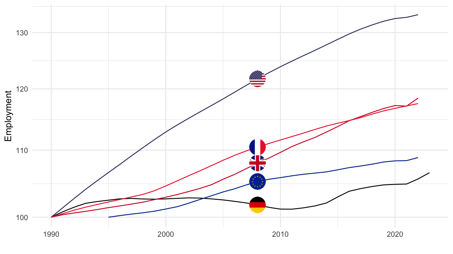

1995-

Code

SNA_TABLE3 %>%
  filter(TRANSACT %in% c("POPNC"),
         MEASURE == "PER",
         LOCATION %in% c("FRA", "DEU", "GBR", "USA", "EA19")) %>%
  year_to_date %>%
  left_join(SNA_TABLE3_var$LOCATION, by = "LOCATION") %>%
  mutate(Location = ifelse(LOCATION == "EA19", "Europe", Location)) %>%
  select(Location, date, TRANSACT, obsValue) %>%
  left_join(colors, by = c("Location" = "country")) %>%
  group_by(Location) %>%
  filter(date >= as.Date("1995-01-01")) %>%
  mutate(obsValue = 100*obsValue/obsValue[1]) %>%
  ggplot() + geom_line(aes(x = date, y = obsValue, color = color)) +
  scale_color_identity() + theme_minimal() + add_5flags +
  scale_x_date(breaks = seq(1920, 2100, 5) %>% paste0("-01-01") %>% as.Date,
               labels = date_format("%Y")) +
  theme(legend.position = c(0.15, 0.9),
        legend.title = element_blank()) +
  scale_y_log10(breaks = seq(100, 300, 5)) +
  ylab("Employment") + xlab("")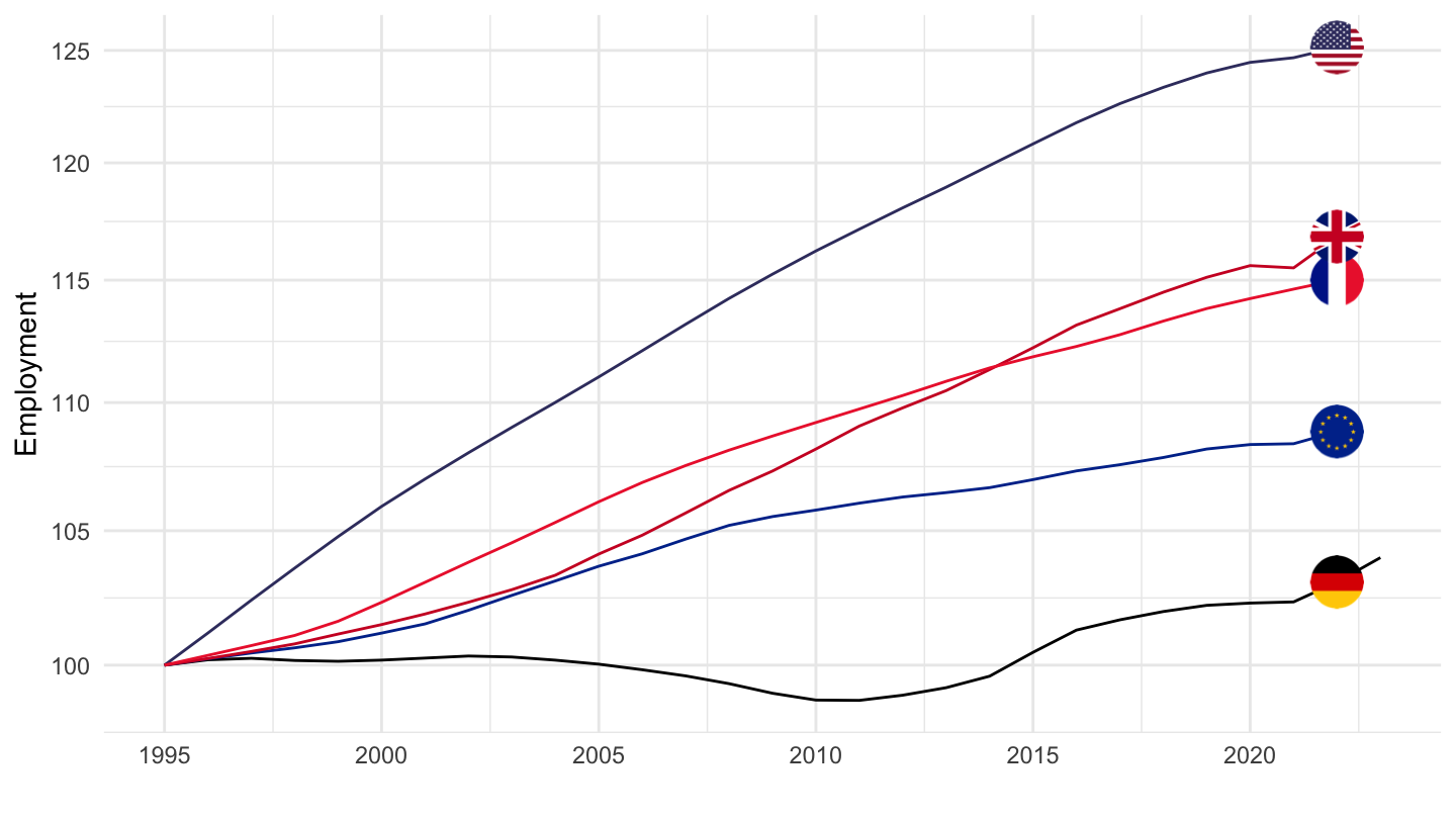

2008-

Code

SNA_TABLE3 %>%
  filter(TRANSACT %in% c("POPNC"),
         MEASURE == "PER",
         LOCATION %in% c("FRA", "DEU", "GBR", "USA", "EA19")) %>%
  year_to_date %>%
  left_join(SNA_TABLE3_var$LOCATION, by = "LOCATION") %>%
  mutate(Location = ifelse(LOCATION == "EA19", "Europe", Location)) %>%
  select(Location, date, TRANSACT, obsValue) %>%
  left_join(colors, by = c("Location" = "country")) %>%
  group_by(Location) %>%
  filter(date >= as.Date("2008-01-01")) %>%
  mutate(obsValue = 100*obsValue/obsValue[1]) %>%
  ggplot() + geom_line(aes(x = date, y = obsValue, color = color)) +
  scale_color_identity() + theme_minimal() + add_5flags +
  scale_x_date(breaks = seq(1920, 2100, 2) %>% paste0("-01-01") %>% as.Date,
               labels = date_format("%Y")) +
  theme(legend.position = c(0.15, 0.9),
        legend.title = element_blank()) +
  scale_y_log10(breaks = seq(100, 300, 1)) +
  ylab("Employment") + xlab("")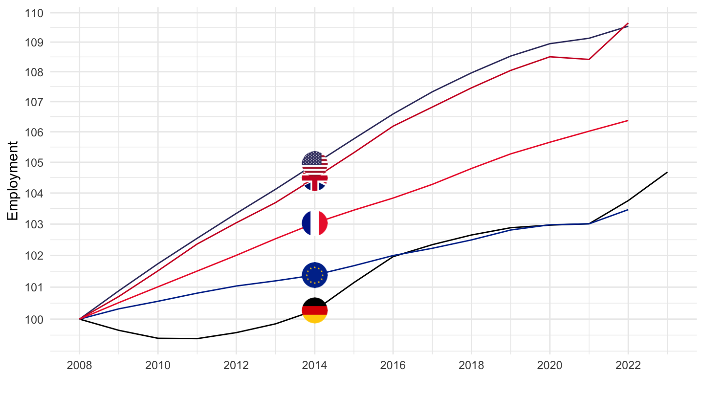

Employment / Population

Number of Persons: PER

All

Code

SNA_TABLE3 %>%
  filter(TRANSACT %in% c("EEM", "POPNC"),
         MEASURE == "PER",
         LOCATION %in% c("FRA", "DEU", "ITA")) %>%
  year_to_date %>%
  left_join(SNA_TABLE3_var$LOCATION, by = "LOCATION") %>%
  select(Location, date, TRANSACT, obsValue) %>%
  spread(TRANSACT, obsValue) %>%
  group_by(Location) %>%
  mutate(POPNC_trend = log(POPNC) %>% hpfilter(1000000) %>% pluck("trend") %>% exp,
         obsValue = EEM / POPNC_trend) %>%
  left_join(colors, by = c("Location" = "country")) %>%
  na.omit %>%
  ggplot() + geom_line(aes(x = date, y = obsValue, color = color)) +
  scale_color_identity() + theme_minimal() + add_3flags +
  scale_x_date(breaks = seq(1920, 2100, 10) %>% paste0("-01-01") %>% as.Date,
               labels = date_format("%Y")) +
  theme(legend.position = c(0.15, 0.9),
        legend.title = element_blank()) +
  scale_y_continuous(breaks = 0.01*seq(-10, 100, 5),
                     labels = scales::percent_format(accuracy = 1)) +
  ylab("Employment / Population") + xlab("")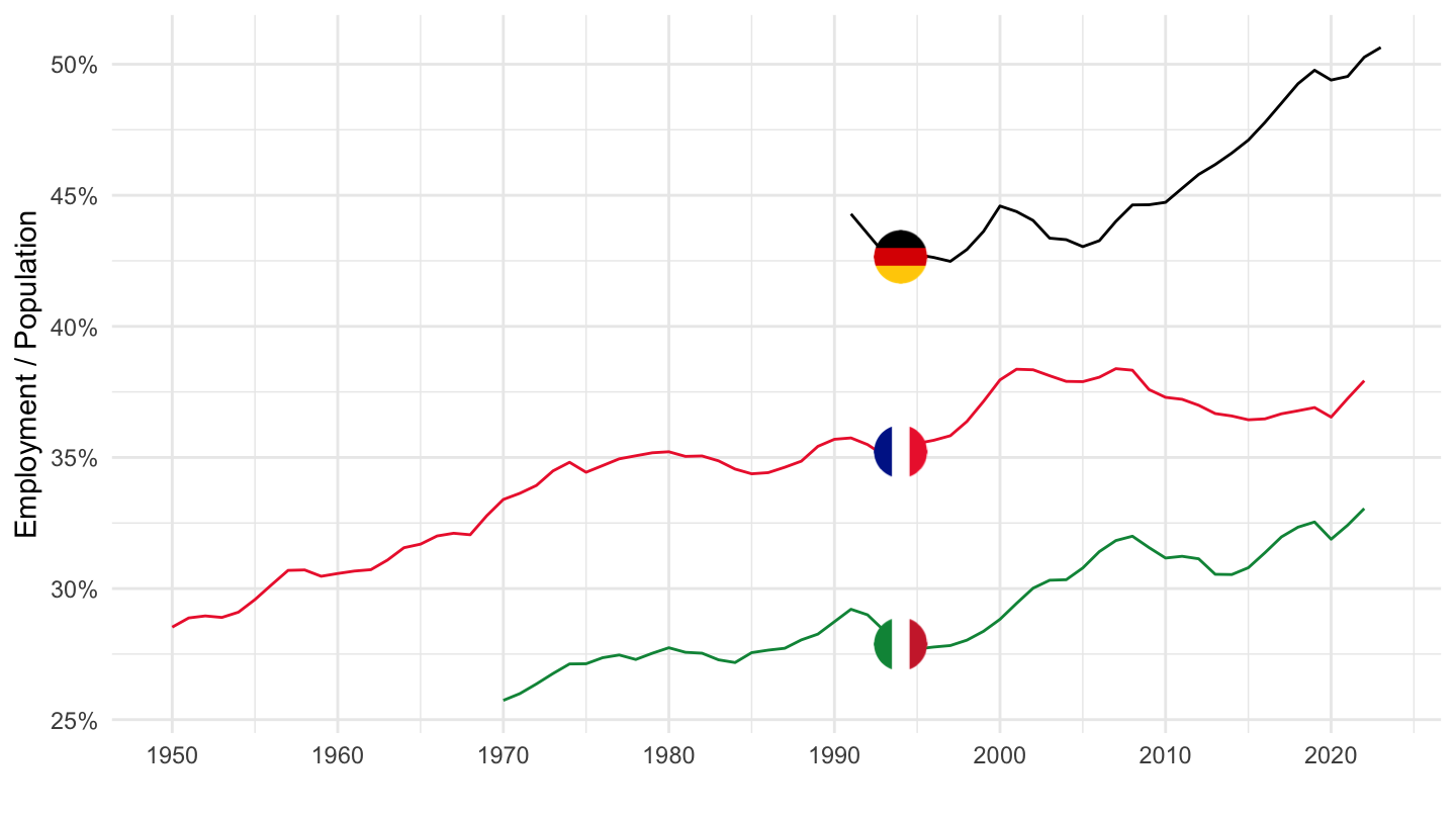

1995-

Code

SNA_TABLE3 %>%
  filter(TRANSACT %in% c("EEM", "POPNC"),
         MEASURE == "PER",
         LOCATION %in% c("FRA", "DEU", "ITA")) %>%
  year_to_date %>%
  filter(date >= as.Date("1995-01-01")) %>%
  left_join(SNA_TABLE3_var$LOCATION, by = "LOCATION") %>%
  select(Location, date, TRANSACT, obsValue) %>%
  spread(TRANSACT, obsValue) %>%
  group_by(Location) %>%
  mutate(POPNC_trend = log(POPNC) %>% hpfilter(1000000) %>% pluck("trend") %>% exp,
         obsValue = EEM / POPNC_trend) %>%
  left_join(colors, by = c("Location" = "country")) %>%
  na.omit %>%
  ggplot() + geom_line(aes(x = date, y = obsValue, color = color)) +
  scale_color_identity() + theme_minimal() + add_3flags +
  scale_x_date(breaks = seq(1920, 2100, 5) %>% paste0("-01-01") %>% as.Date,
               labels = date_format("%Y")) +
  theme(legend.position = c(0.15, 0.9),
        legend.title = element_blank()) +
  scale_y_continuous(breaks = 0.01*seq(-10, 100, 5),
                     labels = scales::percent_format(accuracy = 1)) +
  ylab("Employment / Population") + xlab("")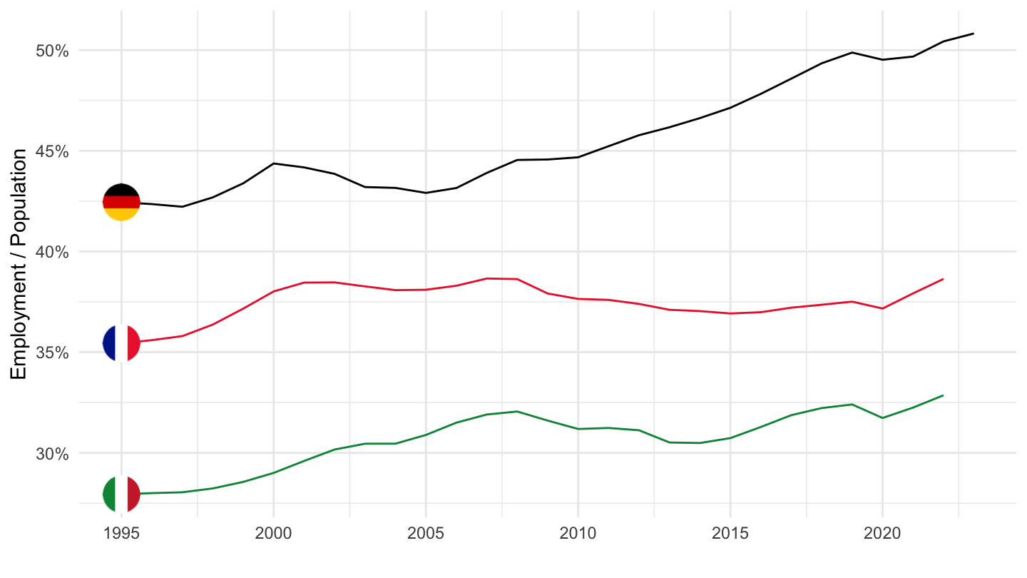

Number of Hours: HRS

All

Code

SNA_TABLE3 %>%
  filter((TRANSACT == "EEM" & MEASURE == "HRS") |
           (TRANSACT == "POPNC" & MEASURE == "PER"),
         LOCATION %in% c("FRA", "DEU", "ITA")) %>%
  year_to_date %>%
  left_join(SNA_TABLE3_var$LOCATION, by = "LOCATION") %>%
  select(Location, date, TRANSACT, obsValue) %>%
  spread(TRANSACT, obsValue) %>%
  group_by(Location) %>%
  mutate(POPNC_trend = log(POPNC) %>% hpfilter(1000000) %>% pluck("trend") %>% exp,
         obsValue = EEM / POPNC_trend) %>%
  left_join(colors, by = c("Location" = "country")) %>%
  na.omit %>%
  ggplot() + geom_line(aes(x = date, y = obsValue, color = color)) +
  scale_color_identity() + theme_minimal() + add_3flags +
  scale_x_date(breaks = seq(1920, 2100, 10) %>% paste0("-01-01") %>% as.Date,
               labels = date_format("%Y")) +
  theme(legend.position = c(0.15, 0.9),
        legend.title = element_blank()) +
  scale_y_continuous(breaks = 0.01*seq(-10, 100, 5),
                     labels = scales::percent_format(accuracy = 1)) +
  ylab("Employment / Population") + xlab("")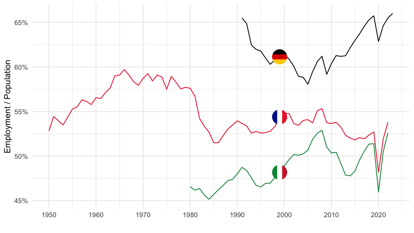

1995-

Code

SNA_TABLE3 %>%
  filter((TRANSACT == "EEM" & MEASURE == "HRS") |
           (TRANSACT == "POPNC" & MEASURE == "PER"),
         LOCATION %in% c("FRA", "DEU", "ITA")) %>%
  year_to_date %>%
  filter(date >= as.Date("1995-01-01")) %>%
  left_join(SNA_TABLE3_var$LOCATION, by = "LOCATION") %>%
  select(Location, date, TRANSACT, obsValue) %>%
  spread(TRANSACT, obsValue) %>%
  group_by(Location) %>%
  mutate(POPNC_trend = log(POPNC) %>% hpfilter(1000000) %>% pluck("trend") %>% exp,
         obsValue = EEM / POPNC_trend) %>%
  left_join(colors, by = c("Location" = "country")) %>%
  na.omit %>%
  ggplot() + geom_line(aes(x = date, y = obsValue, color = color)) +
  scale_color_identity() + theme_minimal() + add_3flags +
  scale_x_date(breaks = seq(1920, 2100, 5) %>% paste0("-01-01") %>% as.Date,
               labels = date_format("%Y")) +
  theme(legend.position = c(0.15, 0.9),
        legend.title = element_blank()) +
  scale_y_continuous(breaks = 0.01*seq(-10, 100, 5),
                     labels = scales::percent_format(accuracy = 1)) +
  ylab("Employment / Population") + xlab("")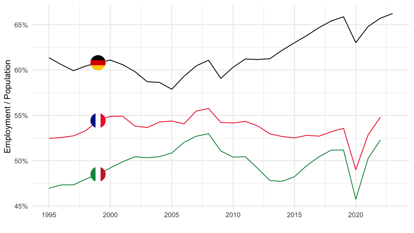

Employment Share Graphs

Industry (B_E)

Code

SNA_TABLE3 %>%
  filter(TRANSACT %in% c("EEMVB_E", "EEM"),
         MEASURE == "PER") %>%
  left_join(SNA_TABLE3_var$LOCATION, by = "LOCATION") %>%
  select(obsTime, LOCATION, Location, TRANSACT, obsValue) %>%
  spread(TRANSACT, obsValue) %>%
  mutate(obsValue = 100*EEMVB_E/EEM) %>%
  na.omit %>%
  group_by(LOCATION, Location) %>%
  summarise(`Year 1` = first(obsTime),
            `Year 2` = last(obsTime),
            `Industry Share 1` = first(obsValue),
            `Industry Share 2` = last(obsValue),
            `Growth (1995-2019)` = obsValue[obsTime == "2019"]/obsValue[obsTime == "1995"]-1,
            `Growth (1980-2019)` = obsValue[obsTime == "2019"]/obsValue[obsTime == "1980"]-1) %>%
  arrange(`Growth (1980-2019)`) %>%
  mutate(Flag = gsub(" ", "-", str_to_lower(gsub(" ", "-", Location))),
         Flag = paste0('<img src="../../icon/flag/vsmall/', Flag, '.png" alt="Flag">')) %>%
  select(Flag, everything()) %>%
  {if (is_html_output()) datatable(., filter = 'top', rownames = F, escape = F) else .}

France, EU 19, EU 28

All

Code

SNA_TABLE3 %>%
  filter((TRANSACT == "EEM" & MEASURE == "PER") |
           (TRANSACT == "EEMVB_E" & MEASURE == "PER"),
         LOCATION %in% c("FRA", "EA19", "EU28")) %>%
  year_to_date %>%
  left_join(SNA_TABLE3_var$LOCATION, by = "LOCATION") %>%
  select(Location, date, TRANSACT, obsValue) %>%
  mutate(Location = ifelse(Location == "Euro area (19 countries)", "Europe", Location)) %>%
  spread(TRANSACT, obsValue) %>%
  group_by(Location) %>%
  mutate(obsValue = EEMVB_E / EEM) %>%
  left_join(colors, by = c("Location" = "country")) %>%
  na.omit %>%
  ggplot() + geom_line(aes(x = date, y = obsValue, color = color)) +
  scale_color_identity() + theme_minimal() + add_2flags +
  theme_minimal() + ylab("Employment Share") + xlab("") +
  scale_x_date(breaks = seq(1920, 2100, 5) %>% paste0("-01-01") %>% as.Date,
               labels = date_format("%Y")) +
  theme(legend.position = c(0.15, 0.2),
        legend.title = element_blank()) +
  scale_y_log10(breaks = 0.01*seq(-10, 100, 2),
                     labels = scales::percent_format(accuracy = 1))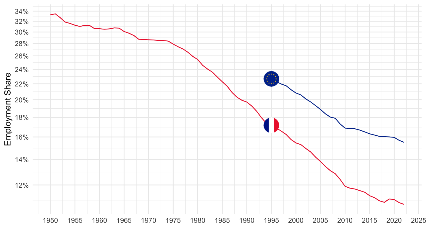

1995-

Code

SNA_TABLE3 %>%
  filter((TRANSACT == "EEM" & MEASURE == "PER") |
           (TRANSACT == "EEMVB_E" & MEASURE == "PER"),
         LOCATION %in% c("FRA", "EA19", "EU28")) %>%
  year_to_date %>%
  filter(date >= as.Date("1995-01-01")) %>%
  left_join(SNA_TABLE3_var$LOCATION, by = "LOCATION") %>%
  select(Location, date, TRANSACT, obsValue) %>%
  mutate(Location = ifelse(Location == "Euro area (19 countries)", "Europe", Location)) %>%
  spread(TRANSACT, obsValue) %>%
  group_by(Location) %>%
  mutate(obsValue = EEMVB_E / EEM) %>%
  left_join(colors, by = c("Location" = "country")) %>%
  na.omit %>%
  ggplot() + geom_line(aes(x = date, y = obsValue, color = color)) +
  scale_color_identity() + theme_minimal() + add_2flags +
  theme_minimal() + ylab("Employment Share") + xlab("") +
  scale_x_date(breaks = seq(1920, 2100, 5) %>% paste0("-01-01") %>% as.Date,
               labels = date_format("%Y")) +
  theme(legend.position = c(0.15, 0.2),
        legend.title = element_blank()) +
  scale_y_log10(breaks = 0.01*seq(-10, 100, 2),
                     labels = scales::percent_format(accuracy = 1))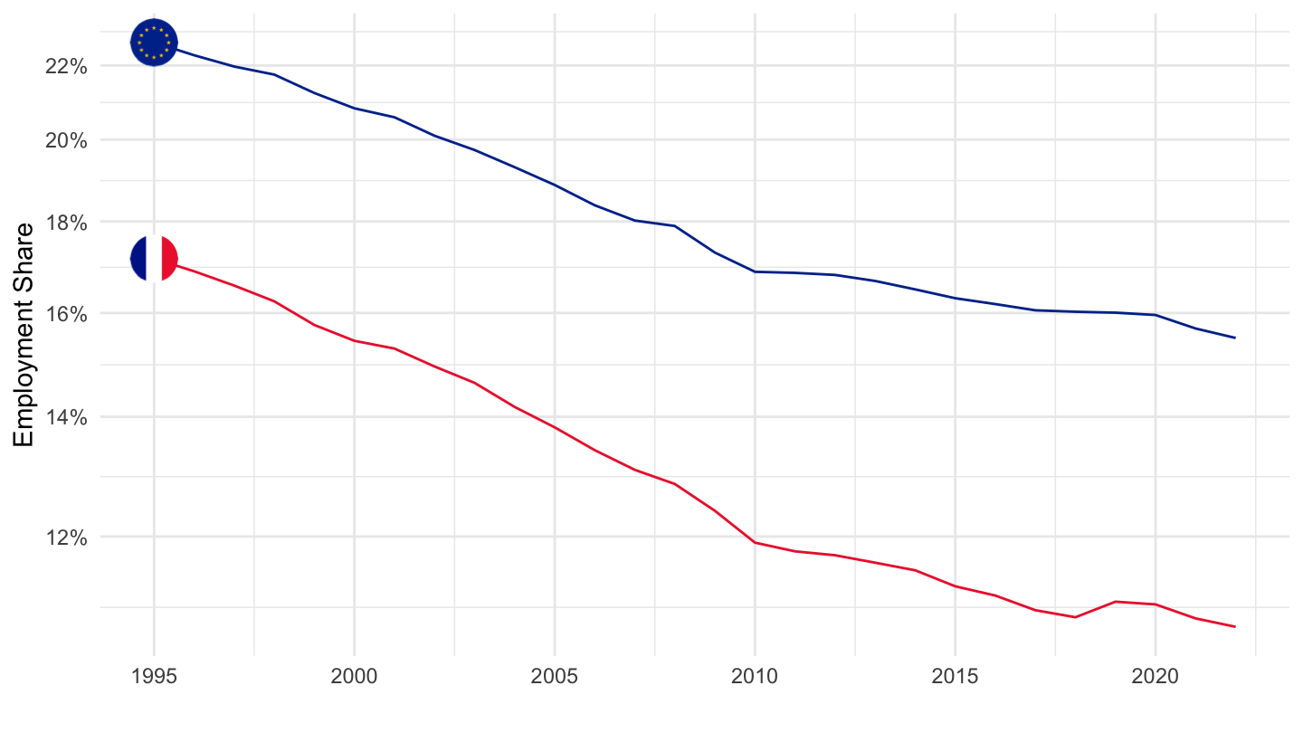

France, Finland

Code

SNA_TABLE3 %>%
  filter((TRANSACT == "EEM" & MEASURE == "PER") |
           (TRANSACT == "EEMVB_E" & MEASURE == "PER"),
         LOCATION %in% c("FRA", "FIN")) %>%
  year_to_date %>%
  filter(date >= as.Date("1970-01-01")) %>%
  left_join(SNA_TABLE3_var$LOCATION, by = "LOCATION") %>%
  select(Location, date, TRANSACT, obsValue) %>%
  spread(TRANSACT, obsValue) %>%
  group_by(Location) %>%
  mutate(obsValue = EEMVB_E / EEM) %>%
  left_join(colors, by = c("Location" = "country")) %>%
  na.omit %>%
  ggplot() + geom_line(aes(x = date, y = obsValue, color = color)) +
  scale_color_identity() + theme_minimal() + add_2flags +
  theme_minimal() + ylab("Employment Share") + xlab("") +
  scale_x_date(breaks = seq(1920, 2100, 5) %>% paste0("-01-01") %>% as.Date,
               labels = date_format("%Y")) +
  theme(legend.position = c(0.15, 0.2),
        legend.title = element_blank()) +
  scale_y_log10(breaks = 0.01*seq(-10, 100, 2),
                     labels = scales::percent_format(accuracy = 1))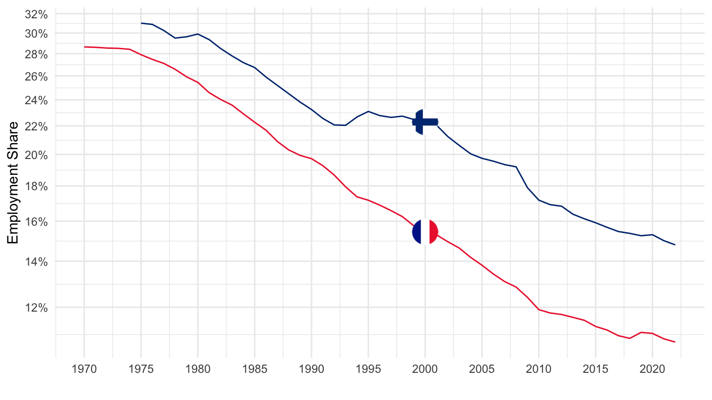

France, Germany, Italy, Spain

All

Code

SNA_TABLE3 %>%
  filter((TRANSACT == "EEM" & MEASURE == "PER") |
           (TRANSACT == "EEMVB_E" & MEASURE == "PER"),
         LOCATION %in% c("FRA", "DEU", "ITA", "ESP")) %>%
  year_to_date %>%
  left_join(SNA_TABLE3_var$LOCATION, by = "LOCATION") %>%
  select(Location, date, TRANSACT, obsValue) %>%
  spread(TRANSACT, obsValue) %>%
  group_by(Location) %>%
  mutate(obsValue = EEMVB_E / EEM) %>%
  left_join(colors, by = c("Location" = "country")) %>%
  na.omit %>%
  ggplot() + geom_line(aes(x = date, y = obsValue, color = color)) +
  scale_color_identity() + theme_minimal() + add_4flags +
  theme_minimal() + ylab("Employment Share") + xlab("") +
  scale_x_date(breaks = seq(1920, 2100, 5) %>% paste0("-01-01") %>% as.Date,
               labels = date_format("%Y")) +
  theme(legend.position = c(0.15, 0.2),
        legend.title = element_blank()) +
  scale_y_log10(breaks = 0.01*seq(-10, 100, 2),
                     labels = scales::percent_format(accuracy = 1))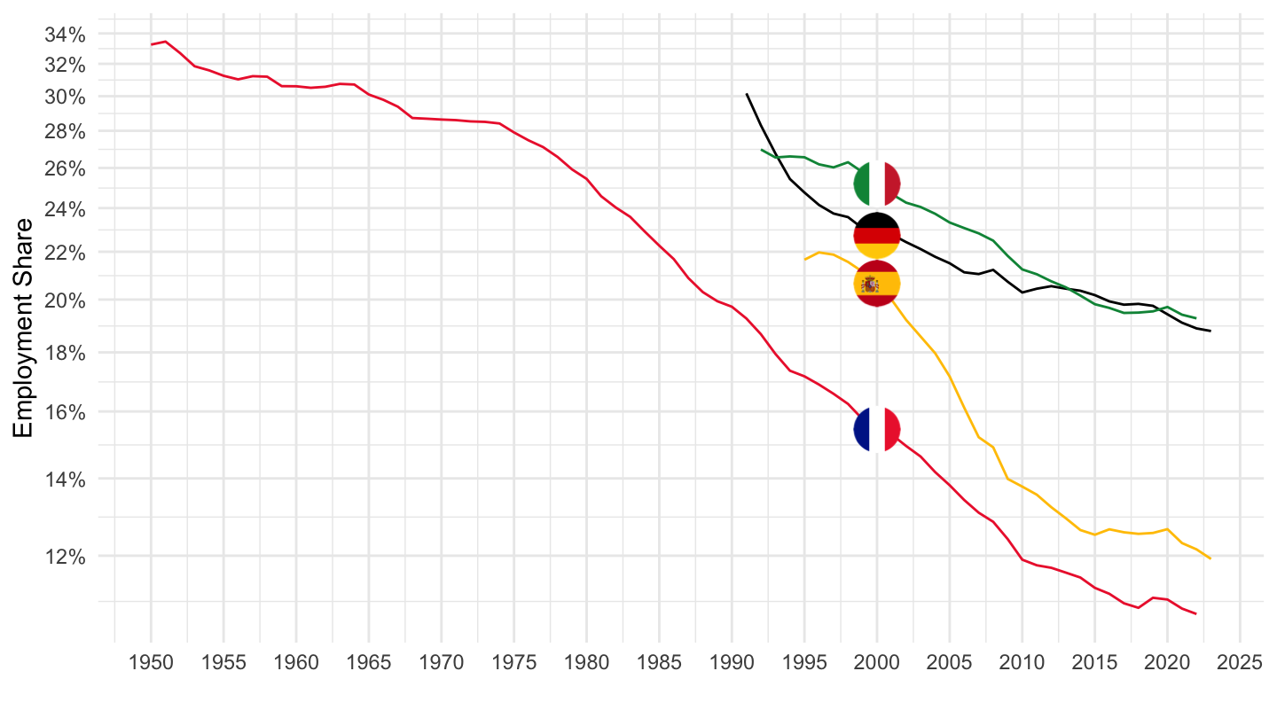

France (1950-2020)

Linear

B-E: Industrie = Manufacturier + Energie

Code

SNA_TABLE3 %>%
  filter((TRANSACT == "EEM" & MEASURE == "PER") |(TRANSACT == "EEMVB_E" & MEASURE == "PER"),
         LOCATION %in% c("FRA")) %>%
  year_to_date %>%
  left_join(SNA_TABLE3_var$LOCATION, by = "LOCATION") %>%
  select(Location, date, TRANSACT, obsValue) %>%
  spread(TRANSACT, obsValue) %>%
  ggplot() + geom_line(aes(x = date, y = EEMVB_E / EEM)) +
  geom_rect(data = data_frame(start = as.Date("1945-01-01"), 
                                end = as.Date("1975-01-01")), 
              aes(xmin = start, xmax = end, ymin = -Inf, ymax = +Inf), fill = viridis(4)[4], alpha = 0.2) +
  theme_minimal() + ylab("Part de l'emploi industriel (%)") + xlab("") +
  scale_x_date(breaks = seq(1925, 2100, 10) %>% paste0("-01-01") %>% as.Date,
               labels = date_format("%Y")) +
  scale_y_continuous(breaks = 0.01*seq(-10, 100, 2),
                labels = scales::percent_format(accuracy = 1))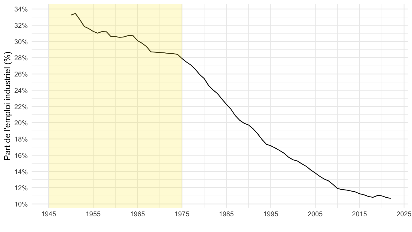

C: Manufacturier

Code

SNA_TABLE3 %>%
  filter((TRANSACT == "EEM" & MEASURE == "PER") |
           (TRANSACT == "EEMVC" & MEASURE == "PER"),
         LOCATION %in% c("FRA")) %>%
  year_to_date %>%
  left_join(SNA_TABLE3_var$LOCATION, by = "LOCATION") %>%
  select(Location, date, TRANSACT, obsValue) %>%
  spread(TRANSACT, obsValue) %>%
  ggplot() + geom_line(aes(x = date, y = EEMVC / EEM)) +
  geom_rect(data = data_frame(start = as.Date("1945-01-01"), 
                                end = as.Date("1975-01-01")), 
              aes(xmin = start, xmax = end, ymin = -Inf, ymax = +Inf), 
              fill = viridis(4)[4], alpha = 0.2) +
  theme_minimal() + ylab("Part de l'emploi manufacturier (%)") + xlab("") +
  scale_x_date(breaks = seq(1925, 2100, 10) %>% paste0("-01-01") %>% as.Date,
               labels = date_format("%Y")) +
  scale_y_continuous(breaks = 0.01*seq(-10, 100, 2),
                labels = scales::percent_format(accuracy = 1))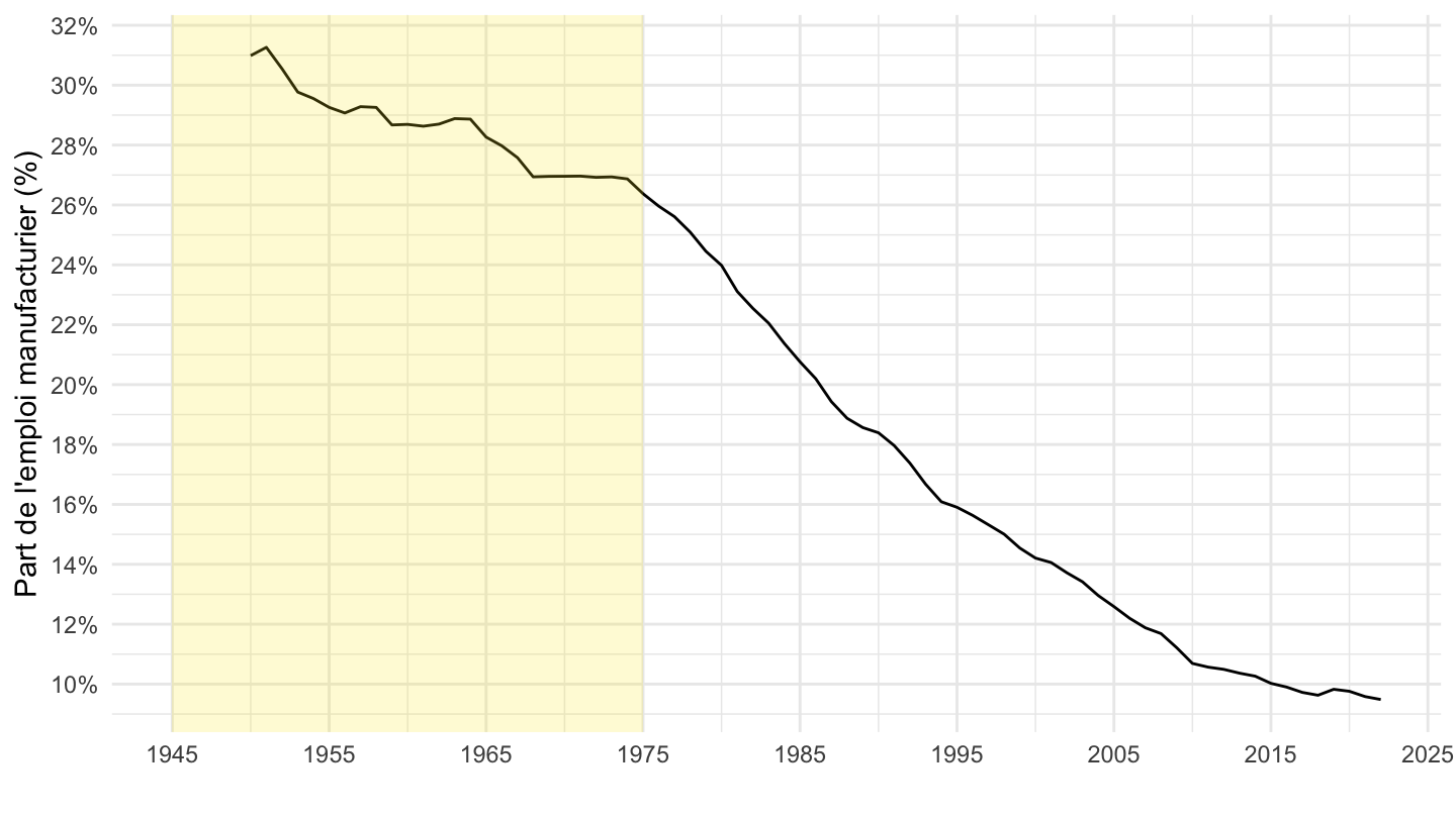

C et B-E

Code

SNA_TABLE3 %>%
  filter((TRANSACT == "EEM" & MEASURE == "PER") |
           (TRANSACT == "EEMVC" & MEASURE == "PER") |
           (TRANSACT == "EEMVB_E" & MEASURE == "PER"),
         LOCATION %in% c("FRA")) %>%
  year_to_date %>%
  left_join(SNA_TABLE3_var$LOCATION, by = "LOCATION") %>%
  select(date, TRANSACT, obsValue) %>%
  spread(TRANSACT, obsValue) %>%
  transmute(date,
            EEMVB_E_EEM = EEMVB_E/EEM,
            EEMVC_EEM = EEMVC/EEM) %>%
  gather(variable, obsValue, -date) %>%
  left_join(tibble(variable = c("EEMVC_EEM", "EEMVB_E_EEM"),
                   Variable = c("Emploi dans le secteur manufacturier en % (C)",
                                "Emploi dans le secteur industriel en % (B-E)")),
            by = "variable") %>%
  ggplot() + geom_line(aes(x = date, y = obsValue, color = Variable)) +
  theme_minimal() + ylab("Part dans l'emploi (%)") + xlab("") +
  geom_rect(data = data_frame(start = as.Date("1945-01-01"), 
                                end = as.Date("1975-01-01")), 
              aes(xmin = start, xmax = end, ymin = -Inf, ymax = +Inf), 
              fill = viridis(3)[3], alpha = 0.2) +
  scale_color_manual(values = viridis(3)[1:2]) +
  theme(legend.position = c(0.75, 0.9),
        legend.title = element_blank()) +
  scale_x_date(breaks = seq(1925, 2100, 10) %>% paste0("-01-01") %>% as.Date,
               labels = date_format("%Y")) +
  scale_y_continuous(breaks = 0.01*seq(-10, 100, 2),
                labels = scales::percent_format(accuracy = 1))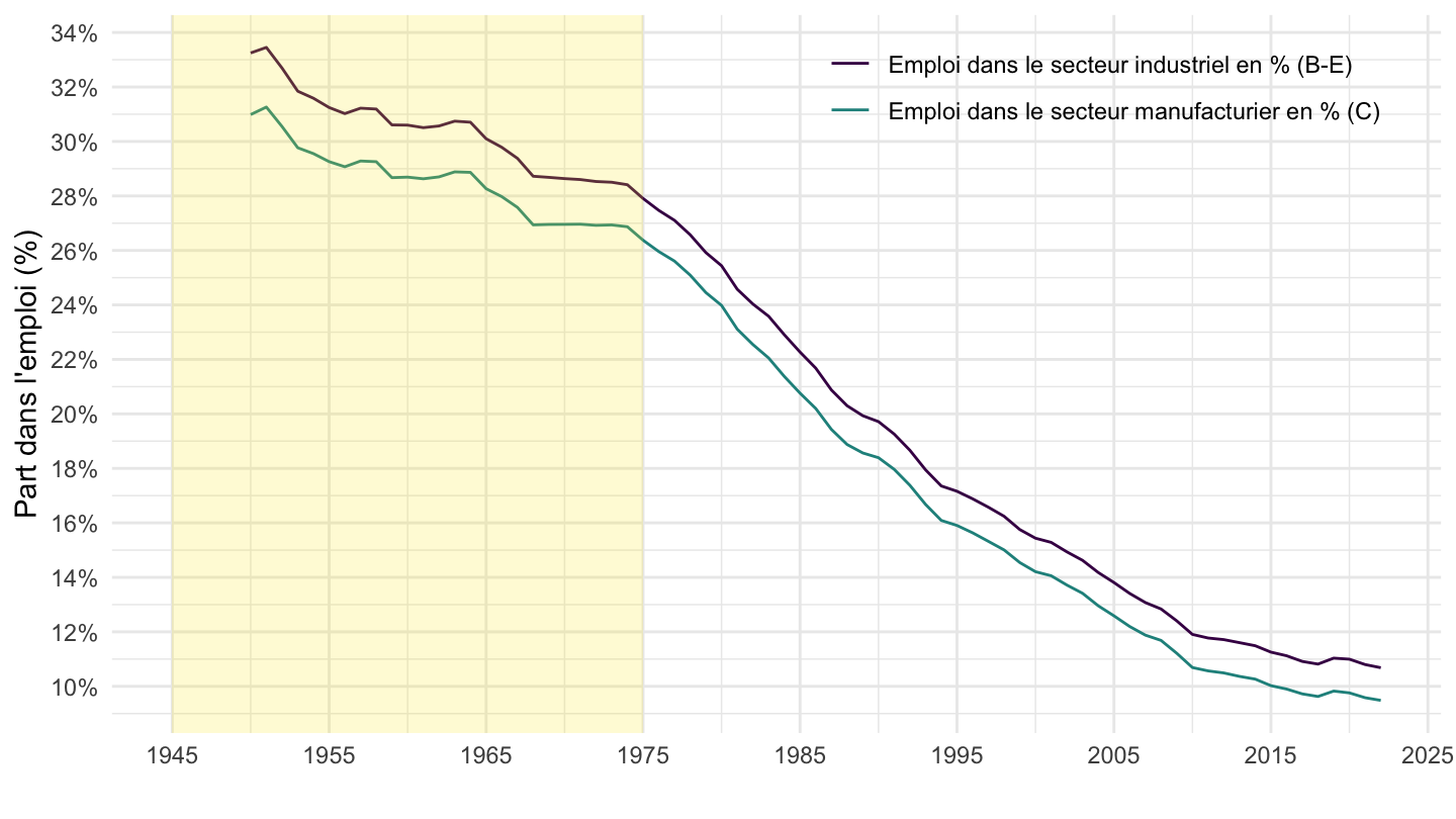

Log

Code

SNA_TABLE3 %>%
  filter((TRANSACT == "EEM" & MEASURE == "PER") |
           (TRANSACT == "EEMVB_E" & MEASURE == "PER"),
         LOCATION %in% c("FRA")) %>%
  year_to_date %>%
  left_join(SNA_TABLE3_var$LOCATION, by = "LOCATION") %>%
  select(Location, date, TRANSACT, obsValue) %>%
  spread(TRANSACT, obsValue) %>%
  ggplot() + geom_line(aes(x = date, y = EEMVB_E / EEM)) +
  theme_minimal() + ylab("Employment Share") + xlab("") +
  scale_x_date(breaks = seq(1920, 2100, 10) %>% paste0("-01-01") %>% as.Date,
               labels = date_format("%Y")) +
  scale_y_log10(breaks = 0.01*seq(-10, 100, 2),
                labels = scales::percent_format(accuracy = 1))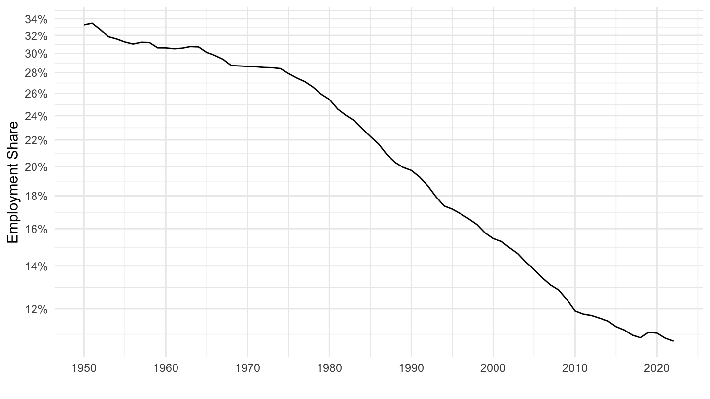

France, Germany, Italy

All

Code

SNA_TABLE3 %>%
  filter((TRANSACT == "EEM" & MEASURE == "PER") |
           (TRANSACT == "EEMVB_E" & MEASURE == "PER"),
         LOCATION %in% c("FRA", "DEU", "ITA")) %>%
  year_to_date %>%
  left_join(SNA_TABLE3_var$LOCATION, by = "LOCATION") %>%
  select(Location, date, TRANSACT, obsValue) %>%
  spread(TRANSACT, obsValue) %>%
  group_by(Location) %>%
  mutate(obsValue = EEMVB_E / EEM) %>%
  left_join(colors, by = c("Location" = "country")) %>%
  na.omit %>%
  ggplot() + geom_line(aes(x = date, y = obsValue, color = color)) +
  scale_color_identity() + theme_minimal() + add_3flags + xlab("") + ylab("") +
  scale_x_date(breaks = seq(1920, 2100, 10) %>% paste0("-01-01") %>% as.Date,
               labels = date_format("%Y")) +
  theme(legend.position = c(0.15, 0.2),
        legend.title = element_blank()) +
  scale_y_continuous(breaks = 0.01*seq(-10, 100, 5),
                     labels = scales::percent_format(accuracy = 1))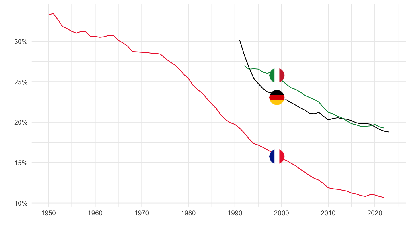

1995-

B-E

Code

SNA_TABLE3 %>%
  filter((TRANSACT == "EEM" & MEASURE == "PER") |
           (TRANSACT == "EEMVB_E" & MEASURE == "PER"),
         LOCATION %in% c("FRA", "DEU", "ITA")) %>%
  year_to_date %>%
  filter(date >= as.Date("1995-01-01")) %>%
  left_join(SNA_TABLE3_var$LOCATION, by = "LOCATION") %>%
  select(Location, date, TRANSACT, obsValue) %>%
  spread(TRANSACT, obsValue) %>%
  group_by(Location) %>%
  mutate(obsValue = EEMVB_E / EEM) %>%
  left_join(colors, by = c("Location" = "country")) %>%
  na.omit %>%
  ggplot() + geom_line(aes(x = date, y = obsValue, color = color)) +
  scale_color_identity() + theme_minimal() + add_3flags +
  theme_minimal() + ylab("Employment Share") + xlab("") +
  scale_x_date(breaks = seq(1920, 2100, 2) %>% paste0("-01-01") %>% as.Date,
               labels = date_format("%Y")) +
  theme(legend.position = c(0.15, 0.2),
        legend.title = element_blank()) +
  scale_y_log10(breaks = 0.01*seq(-10, 100, 2),
                     labels = scales::percent_format(accuracy = 1))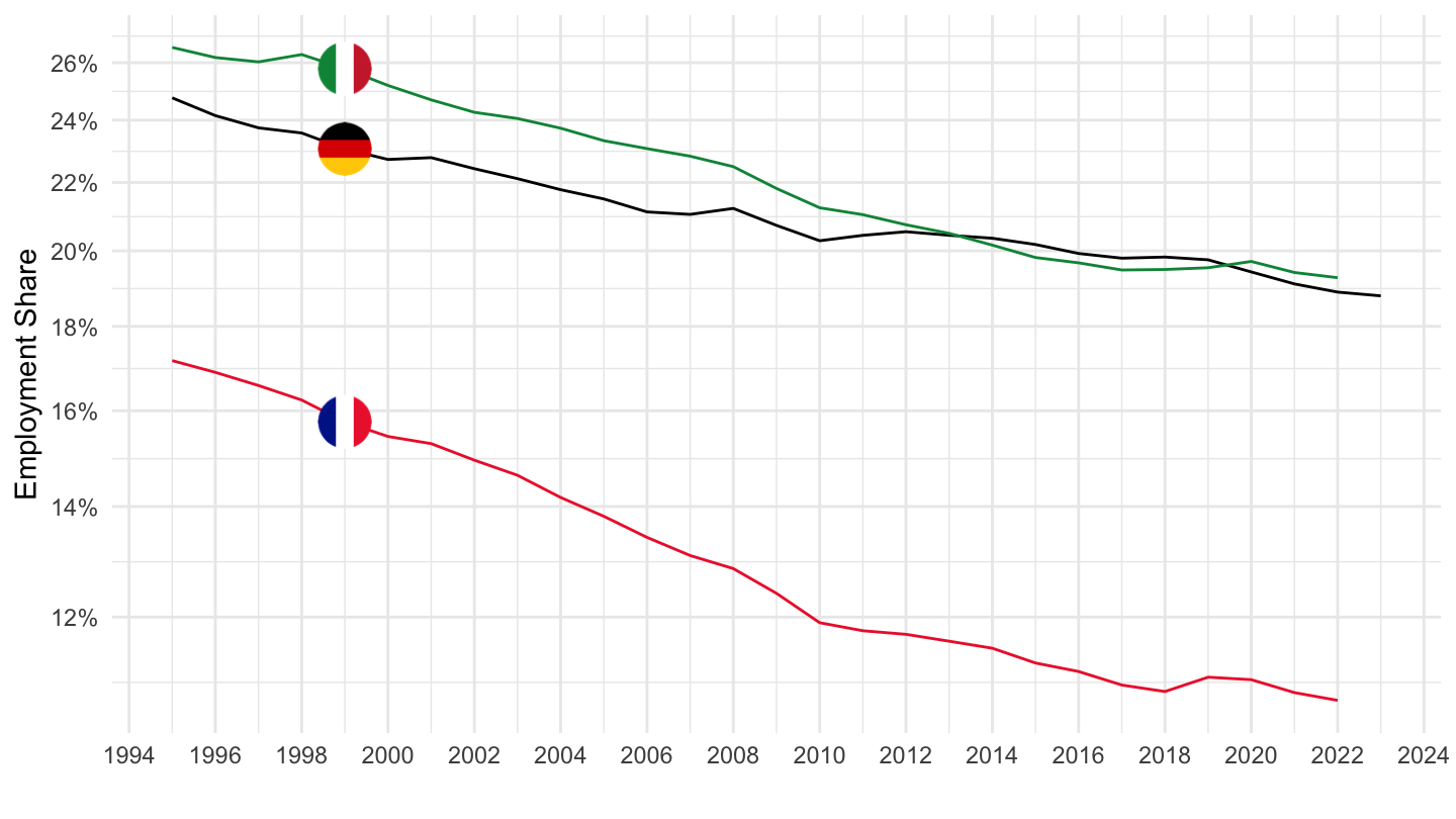

C

Code

SNA_TABLE3 %>%
  filter((TRANSACT == "EEM" & MEASURE == "PER") |
           (TRANSACT == "EEMVC" & MEASURE == "PER"),
         LOCATION %in% c("FRA", "DEU", "ITA")) %>%
  year_to_date %>%
  filter(date >= as.Date("1995-01-01")) %>%
  left_join(SNA_TABLE3_var$LOCATION, by = "LOCATION") %>%
  select(Location, date, TRANSACT, obsValue) %>%
  spread(TRANSACT, obsValue) %>%
  group_by(Location) %>%
  mutate(obsValue = EEMVC / EEM) %>%
  left_join(colors, by = c("Location" = "country")) %>%
  na.omit %>%
  ggplot() + geom_line(aes(x = date, y = obsValue, color = color)) +
  scale_color_identity() + theme_minimal() + add_3flags +
  theme_minimal() + ylab("Employment Share") + xlab("") +
  scale_x_date(breaks = seq(1920, 2100, 2) %>% paste0("-01-01") %>% as.Date,
               labels = date_format("%Y")) +
  theme(legend.position = c(0.15, 0.2),
        legend.title = element_blank()) +
  scale_y_log10(breaks = 0.01*seq(-10, 100, 2),
                     labels = scales::percent_format(accuracy = 1))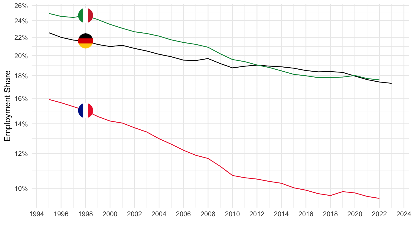

France, Denmark, Netherlands (Low employment)

Code

SNA_TABLE3 %>%
  filter((TRANSACT == "EEM" & MEASURE == "PER") |
           (TRANSACT == "EEMVB_E" & MEASURE == "PER"),
         LOCATION %in% c("FRA", "DNK", "NLD")) %>%
  year_to_date %>%
  left_join(SNA_TABLE3_var$LOCATION, by = "LOCATION") %>%
  select(Location, date, TRANSACT, obsValue) %>%
  spread(TRANSACT, obsValue) %>%
  group_by(Location) %>%
  mutate(obsValue = EEMVB_E / EEM) %>%
  left_join(colors, by = c("Location" = "country")) %>%
  na.omit %>%
  ggplot() + geom_line(aes(x = date, y = obsValue, color = color)) +
  scale_color_identity() + theme_minimal() + add_3flags +
  theme_minimal() + ylab("Employment Share") + xlab("") +
  scale_x_date(breaks = seq(1920, 2100, 5) %>% paste0("-01-01") %>% as.Date,
               labels = date_format("%Y")) +
  theme(legend.position = c(0.15, 0.2),
        legend.title = element_blank()) +
  scale_y_log10(breaks = 0.01*seq(-10, 100, 2),
                     labels = scales::percent_format(accuracy = 1))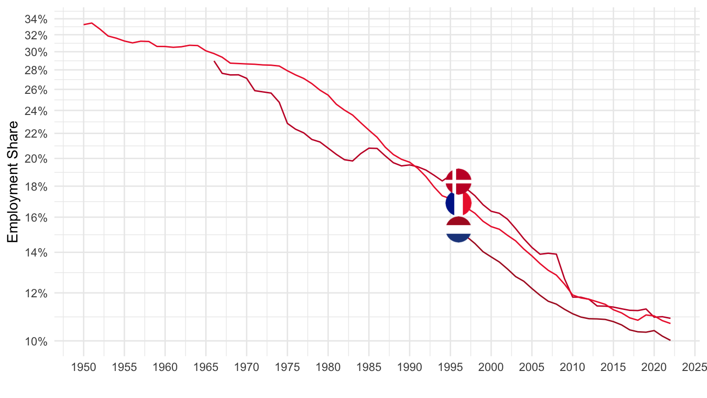

Employment Share Graphs (Hours)

Industry (B_E)

Code

SNA_TABLE3 %>%
  filter(TRANSACT %in% c("EEMVB_E", "EEM"),
         MEASURE == "HRS") %>%
  left_join(SNA_TABLE3_var$LOCATION, by = "LOCATION") %>%
  select(obsTime, LOCATION, Location, TRANSACT, obsValue) %>%
  spread(TRANSACT, obsValue) %>%
  mutate(obsValue = 100*EEMVB_E/EEM) %>%
  na.omit %>%
  group_by(LOCATION, Location) %>%
  summarise(`Year 1` = first(obsTime),
            `Year 2` = last(obsTime),
            `Industry Share 1` = first(obsValue),
            `Industry Share 2` = last(obsValue),
            `Growth (1995-2019)` = obsValue[obsTime == "2019"]/obsValue[obsTime == "1995"]-1,
            `Growth (1980-2019)` = obsValue[obsTime == "2019"]/obsValue[obsTime == "1980"]-1) %>%
  arrange(`Growth (1980-2019)`) %>%
  mutate(Flag = gsub(" ", "-", str_to_lower(gsub(" ", "-", Location))),
         Flag = paste0('<img src="../../icon/flag/vsmall/', Flag, '.png" alt="Flag">')) %>%
  select(Flag, everything()) %>%
  {if (is_html_output()) datatable(., filter = 'top', rownames = F, escape = F) else .}

France, US, UK

Code

SNA_TABLE3 %>%
  filter((TRANSACT == "EEM" & MEASURE == "HRS") |
           (TRANSACT == "EEMVB_E" & MEASURE == "HRS"),
         LOCATION %in% c("FRA", "USA", "GBR")) %>%
  year_to_date %>%
  filter(date >= as.Date("1995-01-01")) %>%
  left_join(SNA_TABLE3_var$LOCATION, by = "LOCATION") %>%
  select(Location, date, TRANSACT, obsValue) %>%
  spread(TRANSACT, obsValue) %>%
  mutate(obsValue = EEMVB_E / EEM) %>%
  left_join(colors, by = c("Location" = "country")) %>%
  ggplot() + geom_line(aes(x = date, y = obsValue, color = color)) +
  scale_color_identity() + theme_minimal() + add_3flags +
  theme_minimal() + ylab("Employment Share") + xlab("") +
  scale_x_date(breaks = seq(1920, 2100, 5) %>% paste0("-01-01") %>% as.Date,
               labels = date_format("%Y")) +
  scale_y_continuous(breaks = 0.01*seq(-10, 100, 1),
                     labels = scales::percent_format(accuracy = 1))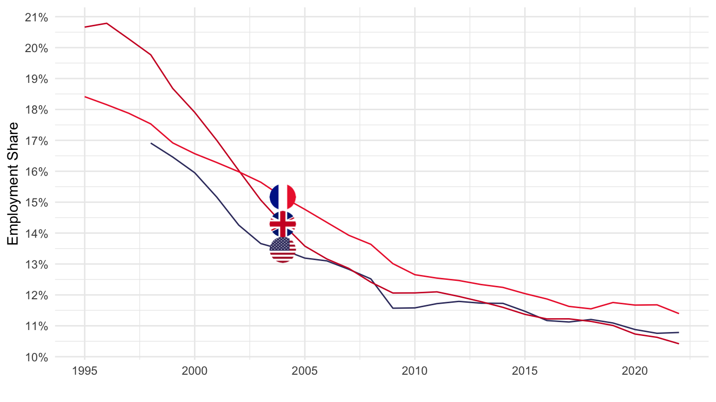

France, EU 19, EU 28

All

Code

SNA_TABLE3 %>%
  filter((TRANSACT == "EEM" & MEASURE == "HRS") |
           (TRANSACT == "EEMVB_E" & MEASURE == "HRS"),
         LOCATION %in% c("FRA", "EA19", "EU28")) %>%
  year_to_date %>%
  left_join(SNA_TABLE3_var$LOCATION, by = "LOCATION") %>%
  mutate(Location = ifelse(Location == "Euro area (19 countries)", "Europe", Location)) %>%
  select(Location, date, TRANSACT, obsValue) %>%
  spread(TRANSACT, obsValue) %>%
  group_by(Location) %>%
  mutate(obsValue = EEMVB_E / EEM) %>%
  left_join(colors, by = c("Location" = "country")) %>%
  na.omit %>%
  ggplot() + geom_line(aes(x = date, y = obsValue, color = color)) +
  scale_color_identity() + theme_minimal() + add_2flags +
  theme_minimal() + ylab("Employment Share") + xlab("") +
  scale_x_date(breaks = seq(1920, 2100, 5) %>% paste0("-01-01") %>% as.Date,
               labels = date_format("%Y")) +
  theme(legend.position = c(0.15, 0.2),
        legend.title = element_blank()) +
  scale_y_log10(breaks = 0.01*seq(-10, 100, 2),
                     labels = scales::percent_format(accuracy = 1))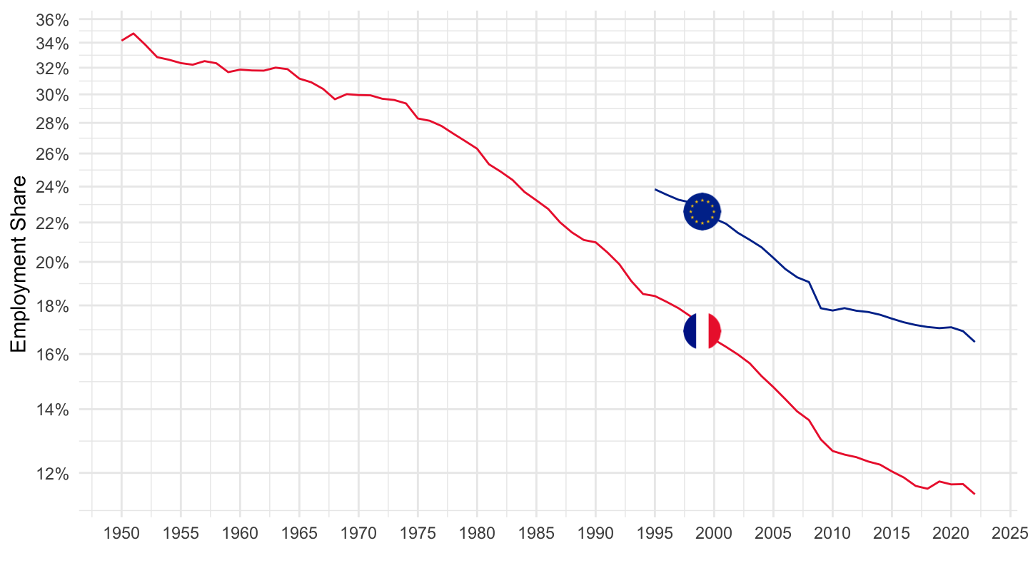

1995-

Code

SNA_TABLE3 %>%
  filter((TRANSACT == "EEM" & MEASURE == "HRS") |
           (TRANSACT == "EEMVB_E" & MEASURE == "HRS"),
         LOCATION %in% c("FRA", "EA19", "EU28")) %>%
  year_to_date %>%
  filter(date >= as.Date("1995-01-01")) %>%
  left_join(SNA_TABLE3_var$LOCATION, by = "LOCATION") %>%
  select(Location, date, TRANSACT, obsValue) %>%
  spread(TRANSACT, obsValue) %>%
  group_by(Location) %>%
  mutate(Location = ifelse(Location == "Euro area (19 countries)", "Europe", Location)) %>%
  mutate(obsValue = EEMVB_E / EEM) %>%
  left_join(colors, by = c("Location" = "country")) %>%
  na.omit %>%
  ggplot() + geom_line(aes(x = date, y = obsValue, color = color)) +
  scale_color_identity() + theme_minimal() + add_2flags +
  theme_minimal() + ylab("Employment Share") + xlab("") +
  scale_x_date(breaks = seq(1920, 2100, 5) %>% paste0("-01-01") %>% as.Date,
               labels = date_format("%Y")) +
  theme(legend.position = c(0.15, 0.2),
        legend.title = element_blank()) +
  scale_y_log10(breaks = 0.01*seq(-10, 100, 2),
                     labels = scales::percent_format(accuracy = 1))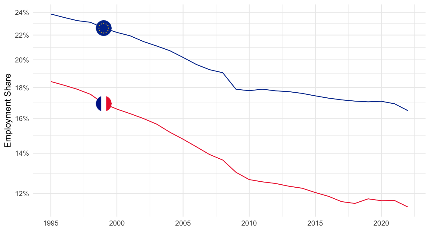

France, Finland

Code

SNA_TABLE3 %>%
  filter((TRANSACT == "EEM" & MEASURE == "HRS") |
           (TRANSACT == "EEMVB_E" & MEASURE == "HRS"),
         LOCATION %in% c("FRA", "FIN")) %>%
  year_to_date %>%
  filter(date >= as.Date("1970-01-01")) %>%
  left_join(SNA_TABLE3_var$LOCATION, by = "LOCATION") %>%
  select(Location, date, TRANSACT, obsValue) %>%
  spread(TRANSACT, obsValue) %>%
  group_by(Location) %>%
  mutate(obsValue = EEMVB_E / EEM) %>%
  left_join(colors, by = c("Location" = "country")) %>%
  na.omit %>%
  ggplot() + geom_line(aes(x = date, y = obsValue, color = color)) +
  scale_color_identity() + theme_minimal() + add_2flags +
  theme_minimal() + ylab("Employment Share") + xlab("") +
  scale_x_date(breaks = seq(1920, 2100, 5) %>% paste0("-01-01") %>% as.Date,
               labels = date_format("%Y")) +
  theme(legend.position = c(0.15, 0.2),
        legend.title = element_blank()) +
  scale_y_log10(breaks = 0.01*seq(-10, 100, 2),
                     labels = scales::percent_format(accuracy = 1))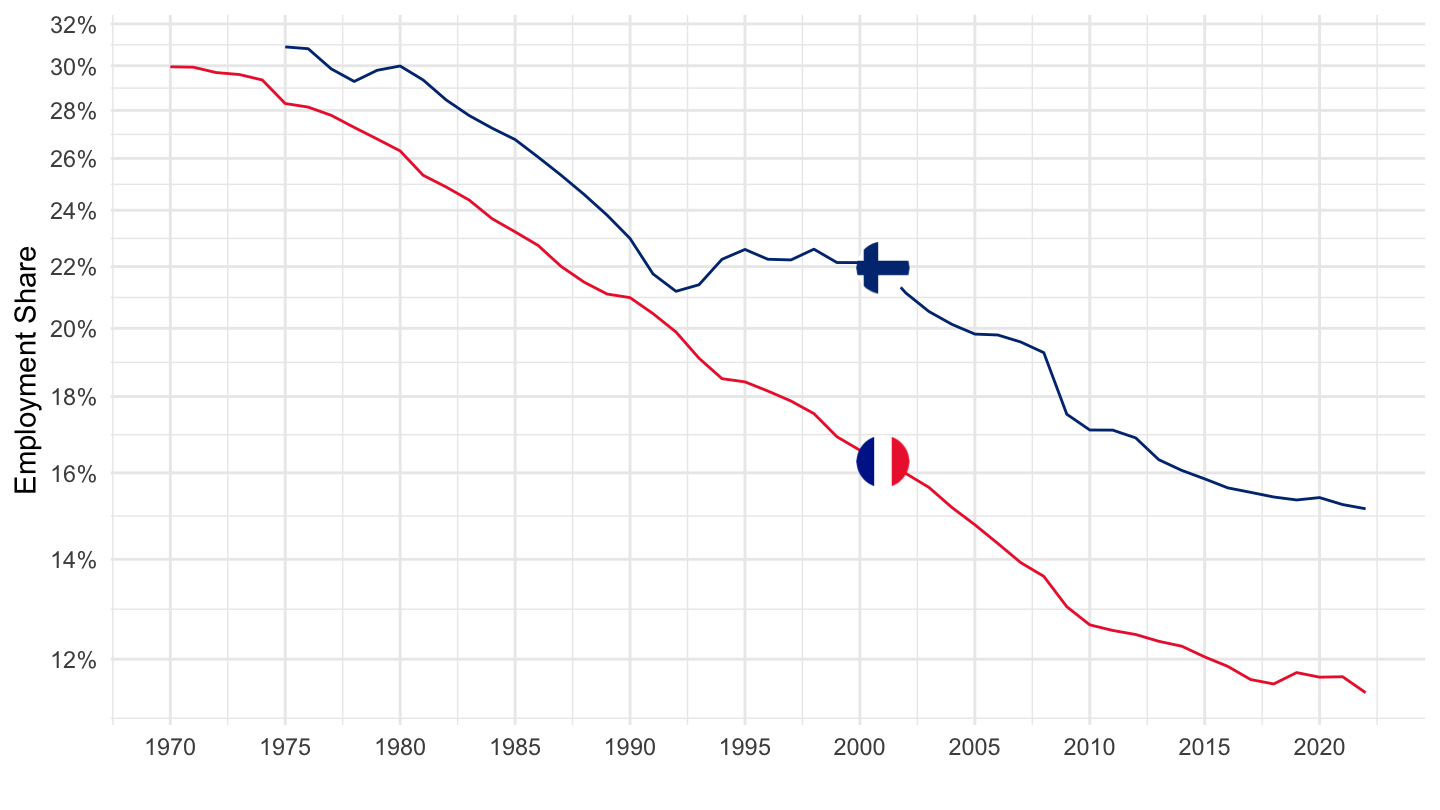

France, Germany, Italy

All

Code

SNA_TABLE3 %>%
  filter((TRANSACT == "EEM" & MEASURE == "HRS") |
           (TRANSACT == "EEMVB_E" & MEASURE == "HRS"),
         LOCATION %in% c("FRA", "DEU", "ITA")) %>%
  year_to_date %>%
  left_join(SNA_TABLE3_var$LOCATION, by = "LOCATION") %>%
  select(Location, date, TRANSACT, obsValue) %>%
  spread(TRANSACT, obsValue) %>%
  group_by(Location) %>%
  mutate(obsValue = EEMVB_E / EEM) %>%
  left_join(colors, by = c("Location" = "country")) %>%
  na.omit %>%
  ggplot() + geom_line(aes(x = date, y = obsValue, color = color)) +
  scale_color_identity() + theme_minimal() + add_3flags +
  theme_minimal() + ylab("Employment Share") + xlab("") +
  scale_x_date(breaks = seq(1920, 2100, 5) %>% paste0("-01-01") %>% as.Date,
               labels = date_format("%Y")) +
  theme(legend.position = c(0.15, 0.2),
        legend.title = element_blank()) +
  scale_y_log10(breaks = 0.01*seq(-10, 100, 2),
                     labels = scales::percent_format(accuracy = 1))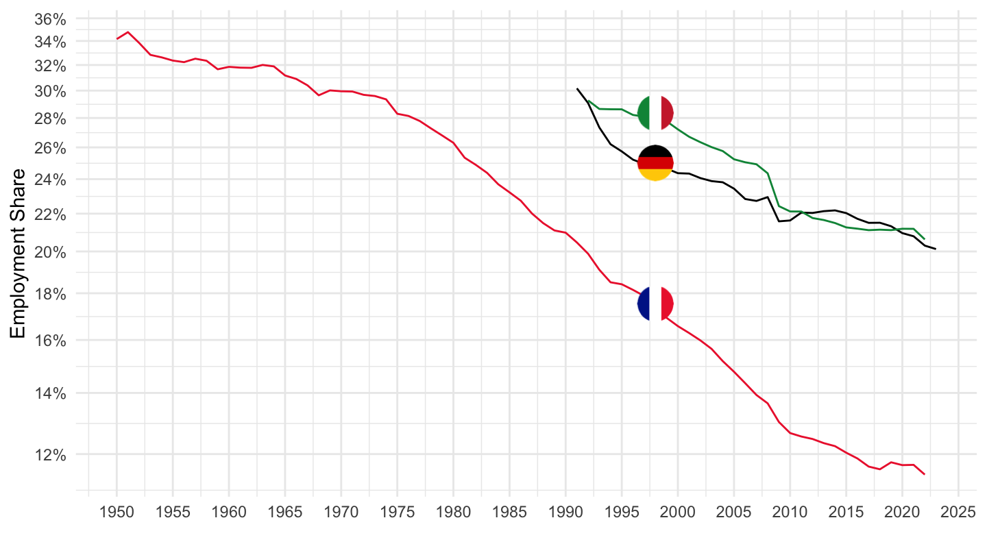

1995-

Code

SNA_TABLE3 %>%
  filter((TRANSACT == "EEM" & MEASURE == "HRS") |
           (TRANSACT == "EEMVB_E" & MEASURE == "HRS"),
         LOCATION %in% c("FRA", "DEU", "ITA")) %>%
  year_to_date %>%
  filter(date >= as.Date("1995-01-01")) %>%
  left_join(SNA_TABLE3_var$LOCATION, by = "LOCATION") %>%
  select(Location, date, TRANSACT, obsValue) %>%
  spread(TRANSACT, obsValue) %>%
  group_by(Location) %>%
  mutate(obsValue = EEMVB_E / EEM) %>%
  left_join(colors, by = c("Location" = "country")) %>%
  na.omit %>%
  ggplot() + geom_line(aes(x = date, y = obsValue, color = color)) +
  scale_color_identity() + theme_minimal() + add_3flags +
  theme_minimal() + ylab("Employment Share") + xlab("") +
  scale_x_date(breaks = seq(1920, 2100, 5) %>% paste0("-01-01") %>% as.Date,
               labels = date_format("%Y")) +
  theme(legend.position = c(0.15, 0.2),
        legend.title = element_blank()) +
  scale_y_log10(breaks = 0.01*seq(-10, 100, 2),
                     labels = scales::percent_format(accuracy = 1))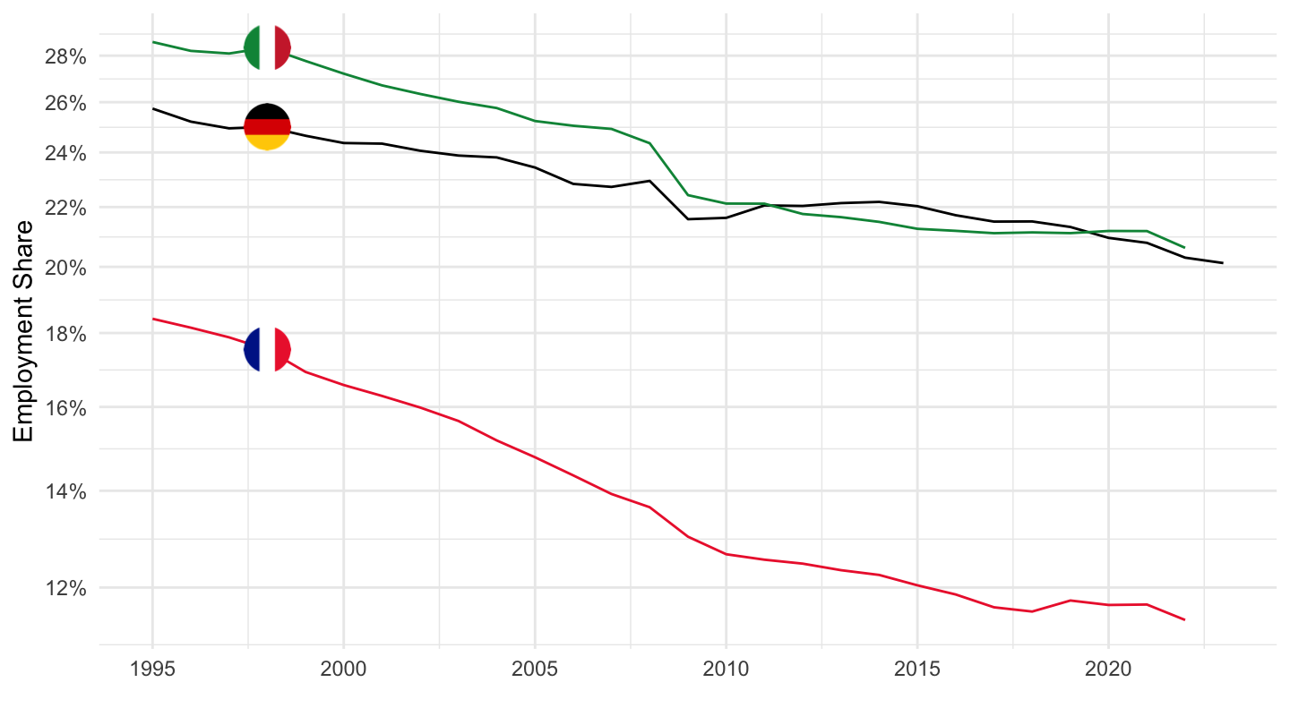

France, Germany, Italy, UK, US

All

Code

SNA_TABLE3 %>%
  filter((TRANSACT == "EEM" & MEASURE == "HRS") |
           (TRANSACT == "EEMVB_E" & MEASURE == "HRS"),
         LOCATION %in% c("FRA", "DEU", "ITA", "USA", "GBR")) %>%
  year_to_date %>%
  left_join(SNA_TABLE3_var$LOCATION, by = "LOCATION") %>%
  select(Location, date, TRANSACT, obsValue) %>%
  spread(TRANSACT, obsValue) %>%
  group_by(Location) %>%
  mutate(obsValue = EEMVB_E / EEM) %>%
  left_join(colors, by = c("Location" = "country")) %>%
  na.omit %>%
  ggplot() + geom_line(aes(x = date, y = obsValue, color = color)) +
  scale_color_identity() + theme_minimal() + add_5flags +
  theme_minimal() + ylab("Employment Share") + xlab("") +
  scale_x_date(breaks = seq(1920, 2100, 5) %>% paste0("-01-01") %>% as.Date,
               labels = date_format("%Y")) +
  theme(legend.position = c(0.15, 0.2),
        legend.title = element_blank()) +
  scale_y_log10(breaks = 0.01*seq(-10, 100, 2),
                     labels = scales::percent_format(accuracy = 1))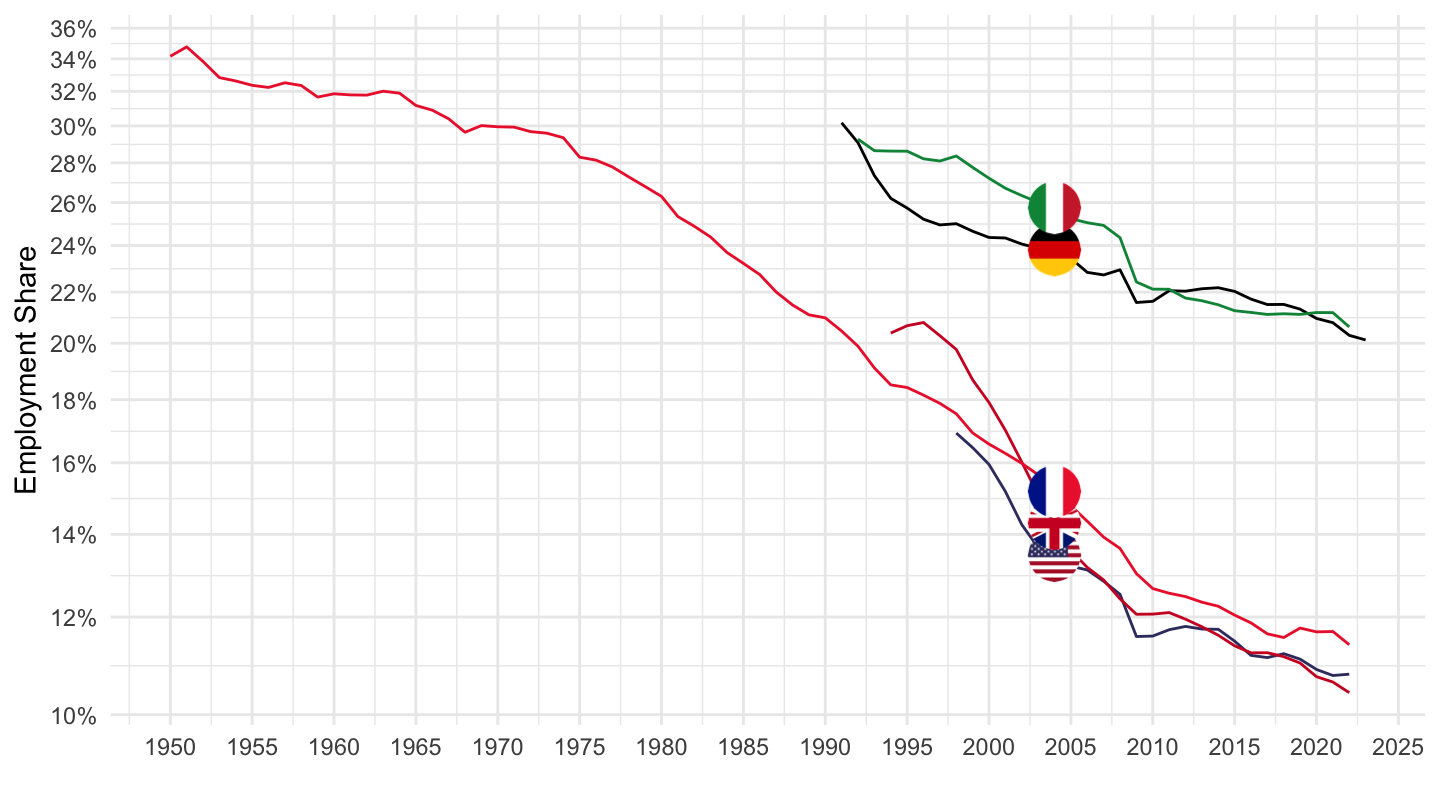

1995-

Code

SNA_TABLE3 %>%
  filter((TRANSACT == "EEM" & MEASURE == "HRS") |
           (TRANSACT == "EEMVB_E" & MEASURE == "HRS"),
         LOCATION %in% c("FRA", "DEU", "ITA", "USA", "GBR")) %>%
  year_to_date %>%
  left_join(SNA_TABLE3_var$LOCATION, by = "LOCATION") %>%
  select(Location, date, TRANSACT, obsValue) %>%
  spread(TRANSACT, obsValue) %>%
  group_by(Location) %>%
  mutate(obsValue = EEMVB_E / EEM) %>%
  left_join(colors, by = c("Location" = "country")) %>%
  na.omit %>%
  filter(date >= as.Date("1995-01-01")) %>%
  ggplot() + geom_line(aes(x = date, y = obsValue, color = color)) +
  scale_color_identity() + theme_minimal() + add_5flags +
  theme_minimal() + ylab("Employment Share") + xlab("") +
  scale_x_date(breaks = seq(1920, 2100, 5) %>% paste0("-01-01") %>% as.Date,
               labels = date_format("%Y")) +
  theme(legend.position = c(0.15, 0.2),
        legend.title = element_blank()) +
  scale_y_log10(breaks = 0.01*seq(-10, 100, 2),
                     labels = scales::percent_format(accuracy = 1))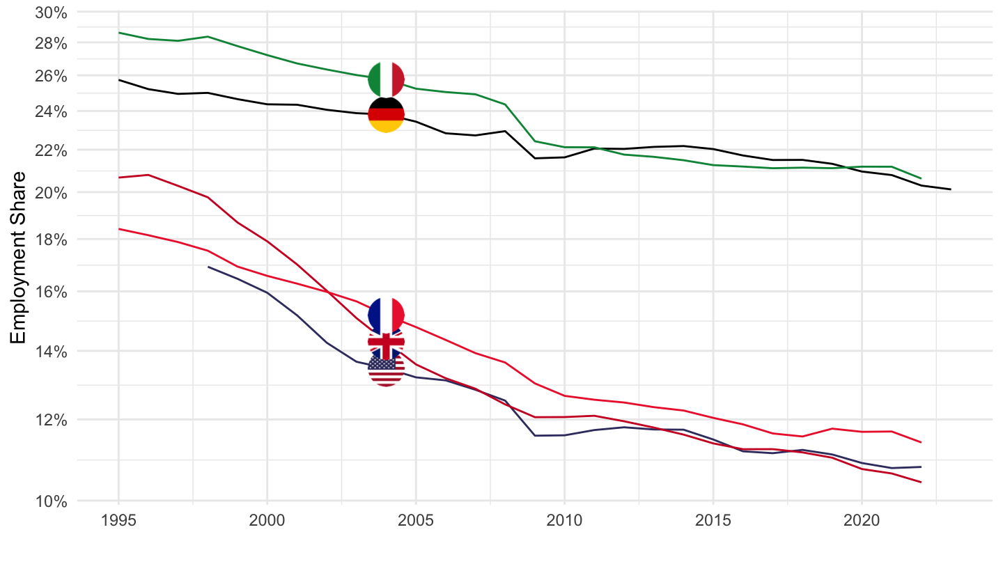

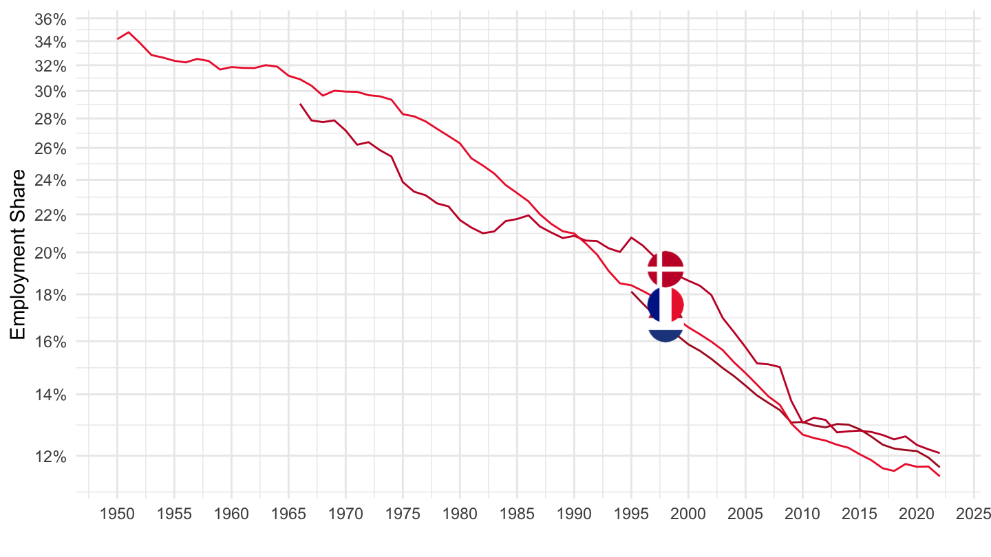
France, Denmark, Netherlands

Code

SNA_TABLE3 %>%
  filter((TRANSACT == "EEM" & MEASURE == "HRS") |
           (TRANSACT == "EEMVB_E" & MEASURE == "HRS"),
         LOCATION %in% c("FRA", "DNK", "NLD")) %>%
  year_to_date %>%
  left_join(SNA_TABLE3_var$LOCATION, by = "LOCATION") %>%
  select(Location, date, TRANSACT, obsValue) %>%
  spread(TRANSACT, obsValue) %>%
  group_by(Location) %>%
  mutate(obsValue = EEMVB_E / EEM) %>%
  left_join(colors, by = c("Location" = "country")) %>%
  na.omit %>%
  ggplot() + geom_line(aes(x = date, y = obsValue, color = color)) +
  scale_color_identity() + theme_minimal() + add_3flags +
  theme_minimal() + ylab("Employment Share") + xlab("") +
  scale_x_date(breaks = seq(1920, 2100, 5) %>% paste0("-01-01") %>% as.Date,
               labels = date_format("%Y")) +
  theme(legend.position = c(0.15, 0.2),
        legend.title = element_blank()) +
  scale_y_log10(breaks = 0.01*seq(-10, 100, 2),
                     labels = scales::percent_format(accuracy = 1))