
Last observation: 9 oct. 2026 (N = 6)
First observation: 1 oct. 2019 (N = 10)
Last data update: 09 oct. 2026, 22:25
Last compile: 10 oct. 2026, 01:47
The €STR is the overnight rate at which euro area banks actually lend to each other, and it is the anchor for the “compounded average rates” (1w, 1m, 3m, 6m, 1y) also published in this dataset.
Since 2019, the ECB has steered it through a corridor system: the deposit facility rate (floor), the main refinancing rate, and the marginal lending facility rate (ceiling). The chart below shows how closely the €STR tracks the deposit facility rate - the key channel through which ECB policy decisions are transmitted to money markets.
Note the €STR consistently trades below the deposit facility rate, by about 6–9 basis points throughout the whole series. This is a well-known feature: money market funds and other non-bank lenders, who can’t park cash at the ECB’s deposit facility, are willing to lend unsecured overnight below the DFR rather than not at all, which pulls the €STR fixing slightly under the floor.
series_levels <- c("ECB Marginal lending facility (ceiling)",
                    "ECB Main refinancing rate",
                    "ECB Deposit facility rate (floor)",
                    "€STR (Euro short-term rate)")

corridor <- FM |>
  filter(PROVIDER_FM_ID %in% c("DFR", "MRR_RT", "MLFR"),
         DATA_TYPE_FM == "LEV",
         FREQ == "D") |>
  day_to_date() |>
  transmute(date, OBS_VALUE,
            series = factor(PROVIDER_FM_ID,
                             levels = c("MLFR", "MRR_RT", "DFR"),
                             labels = c("ECB Marginal lending facility (ceiling)",
                                        "ECB Main refinancing rate",
                                        "ECB Deposit facility rate (floor)")))

estr <- EST |>
  filter(DATA_TYPE_EST == "WT") |>
  day_to_date() |>
  transmute(date, OBS_VALUE, series = "€STR (Euro short-term rate)")

bind_rows(corridor, estr) |>
  mutate(series = factor(series, levels = series_levels)) |>
  ggplot() +
  geom_line(aes(x = date, y = OBS_VALUE / 100, color = series,
                linewidth = series == "€STR (Euro short-term rate)")) +
  scale_linewidth_manual(values = c(`TRUE` = 1, `FALSE` = 0.4), guide = "none") +
  theme_minimal() + xlab("") + ylab("Interest rates (%)") +
  scale_x_date(breaks = seq(1900, 2100, 5) |> paste0("-01-01") |> as.Date(),
               labels = date_format("%Y")) +
  scale_y_continuous(labels = percent_format(accuracy = 0.1)) +
  theme(legend.position = c(0.2, 0.8),
        legend.title = element_blank())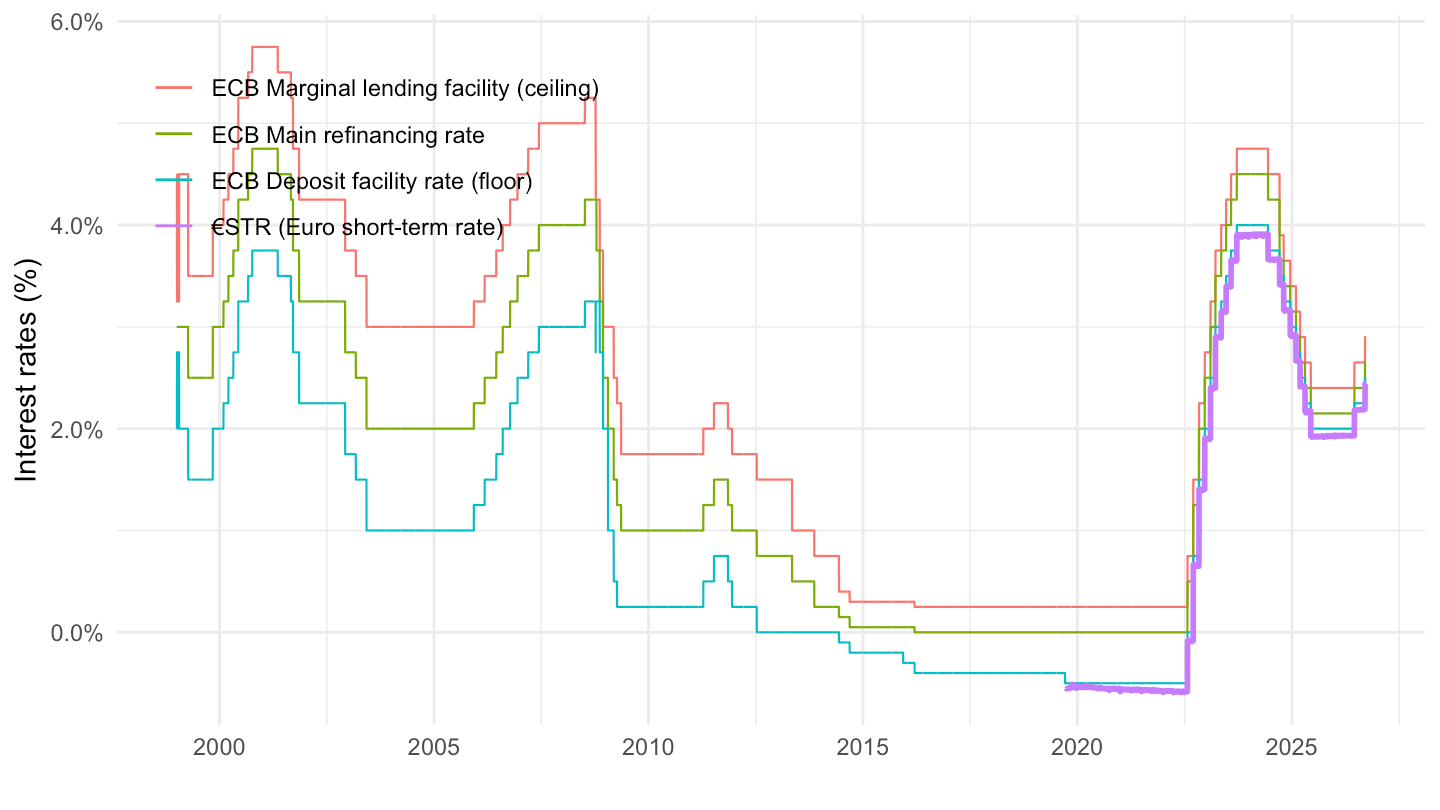
bind_rows(corridor, estr) |>
  filter(date >= as.Date("2019-10-01")) |>
  mutate(series = factor(series, levels = series_levels)) |>
  ggplot() +
  geom_line(aes(x = date, y = OBS_VALUE / 100, color = series,
                linewidth = series == "€STR (Euro short-term rate)")) +
  scale_linewidth_manual(values = c(`TRUE` = 1, `FALSE` = 0.4), guide = "none") +
  theme_minimal() + xlab("") + ylab("Interest rates (%)") +
  scale_x_date(breaks = seq(2019, 2100, 1) |> paste0("-01-01") |> as.Date(),
               labels = date_format("%Y")) +
  scale_y_continuous(labels = percent_format(accuracy = 0.1)) +
  theme(legend.position = c(0.25, 0.8),
        legend.title = element_blank())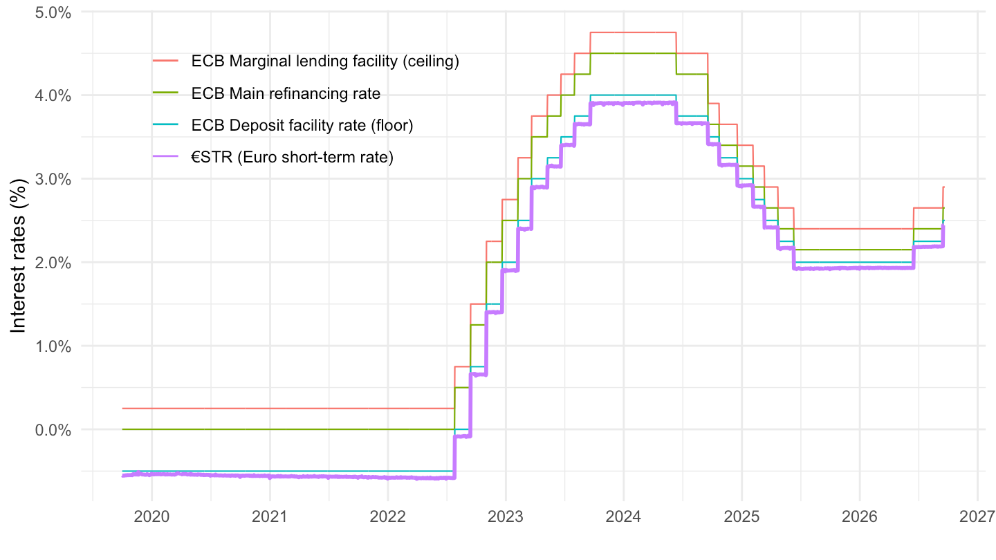
bind_rows(corridor, estr) |>
  filter(date >= as.Date("2022-01-01")) |>
  mutate(series = factor(series, levels = series_levels)) |>
  ggplot() +
  geom_line(aes(x = date, y = OBS_VALUE / 100, color = series,
                linewidth = series == "€STR (Euro short-term rate)")) +
  scale_linewidth_manual(values = c(`TRUE` = 1, `FALSE` = 0.4), guide = "none") +
  theme_minimal() + xlab("") + ylab("Interest rates (%)") +
  scale_x_date(breaks = seq(1960, 2100, 1) |> paste0("-01-01") |> as.Date(),
               labels = date_format("%Y")) +
  scale_y_continuous(breaks = 0.0025*seq(-40, 400, 2),
                     labels = percent_format(accuracy = 0.1)) +
  theme(legend.position = c(0.7, 0.25),
        legend.title = element_blank())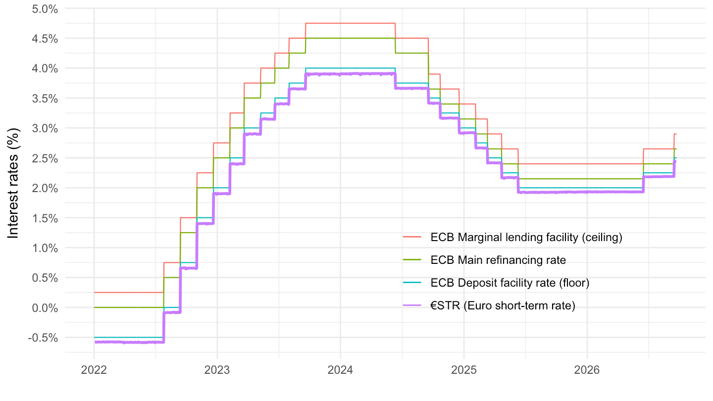
| source | dataset | Title | Updated |
|---|---|---|---|


