Last observation: 2020 (N = 6602)
First observation: 1988 (N = 2168)
Last data update: 09 sept. 2026, 07:40
Last compile: 09 oct. 2026, 22:22
hbs_str_t225 |>
  filter(time == "2020",
         geo == "FR") %>%

  select_if(~ n_distinct(.) > 1) |>
  spread(age, values) %>%
  select_if(~ n_distinct(.) > 1) |>
print_table_conditional()hbs_str_t225 |>
filter(time == "2015",
geo == "FR") %>%
select_if(~ n_distinct(.) > 1) |>
spread(age, values) %>%
select_if(~ n_distinct(.) > 1) |>
print_table_conditional()hbs_str_t225 |>
filter(time == "2015",
geo == "FR",
nchar(coicop) == 4) %>%
select_if(~ n_distinct(.) > 1) |>
spread(age, values) %>%
select_if(~ n_distinct(.) > 1) |>
print_table_conditional()hbs_str_t225 |>
filter(time == "2020",
substr(coicop, 1, 2) == "CP",
nchar(coicop) == 4) %>%
select_if(~ n_distinct(.) > 1) |>
group_by(age, geo, Geo) |>
summarise(values = sum(values)) |>
spread(age, values) |>
print_table_conditional()hbs_str_t225 |>
filter(time == "2020",
substr(coicop, 1, 2) == "CP",
nchar(coicop) == 5) %>%
select_if(~ n_distinct(.) > 1) |>
group_by(age, geo, Geo) |>
summarise(values = sum(values)) |>
spread(age, values) |>
print_table_conditional()| geo | Geo | UNK | Y_GE60 | Y_LT30 | Y30-44 | Y45-59 |
|---|---|---|---|---|---|---|
| AT | Austria | NA | 1000 | 1001 | 999 | 1001 |
| BE | Belgium | NA | 998 | 1002 | 995 | 1001 |
| BG | Bulgaria | NA | 1000 | 1000 | 998 | 999 |
| CY | Cyprus | NA | 994 | 1001 | 998 | 996 |
| CZ | Czechia | NA | 1000 | 1003 | 998 | 998 |
| DE | Germany | NA | 996 | 977 | 990 | 986 |
| DK | Denmark | NA | 995 | 998 | 1000 | 1002 |
| EE | Estonia | NA | 983 | 979 | 984 | 989 |
| EL | Greece | NA | 1001 | 1001 | 1001 | 1001 |
| ES | Spain | NA | 1000 | 1000 | 1002 | 999 |
| FI | Finland | NA | 990 | 973 | 973 | 979 |
| FR | France | NA | 986 | 991 | 989 | 983 |
| HR | Croatia | NA | 1000 | NA | 1000 | 1003 |
| HU | Hungary | NA | 997 | 999 | 999 | 1004 |
| IE | Ireland | NA | 1002 | 1002 | 1003 | 1000 |
| IT | Italy | NA | 1001 | 1000 | 1000 | 997 |
| LT | Lithuania | NA | 1000 | 999 | 1001 | 999 |
| LU | Luxembourg | NA | 999 | 998 | 1000 | 998 |
| LV | Latvia | NA | 998 | 1000 | 996 | 1000 |
| ME | Montenegro | NA | 985 | NA | 983 | 985 |
| MT | Malta | NA | 1002 | 1001 | 1001 | 1000 |
| NL | Netherlands | NA | 1002 | 1002 | 1002 | 998 |
| NO | Norway | NA | 998 | 981 | 995 | 996 |
| PL | Poland | NA | 998 | 1002 | 996 | 999 |
| RS | Serbia | NA | 998 | 999 | 1001 | 998 |
| SI | Slovenia | NA | 1000 | 1001 | 1000 | 1000 |
| SK | Slovakia | NA | 1001 | 999 | 998 | 998 |
| TR | Türkiye | NA | 1001 | 1001 | 1000 | 998 |
hbs_str_t225 |>
  filter(coicop %in% c("CP041", "CP042"),
         time == "2015",
         geo %in% c("FR")) |>
  spread(coicop, values) |>
  mutate(CP041_042 = CP041 + CP042) |>
  gather(coicop, values, CP041, CP042, CP041_042) |>


  add_flag_color("Geo") |>
  mutate(Coicop = ifelse(coicop == "CP041_042", "Imputed rentals plus actual rentals", Coicop),
         age = ifelse(age == "Y_GE60", "Y60+", age),
         age = ifelse(age == "Y_LT30", "Y30-", age)) |>
  ggplot() + geom_line(aes(x = age, y = values/1000, color = Coicop, group = Coicop)) +
  theme_minimal() +
  xlab("") + ylab("Weight in CPI") +
  scale_y_continuous(breaks = 0.01*seq(-30, 50, 2),
                     labels = percent_format(accuracy = 1)) +
  theme(legend.position = c(0.2, 0.9),
        legend.title = element_blank())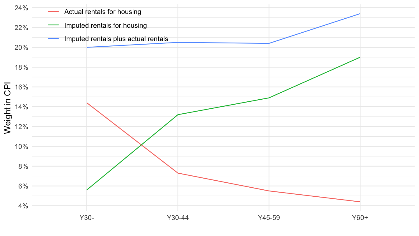
hbs_str_t225 |>
  filter(coicop %in% c("CP041", "CP042"),
         time == "2015",
         geo %in% c("FR")) |>
  mutate(Coicop = factor(coicop, levels = c("CP042", "CP041"), labels = c("Loyers imputés (propriétaires)", "Loyers réels (locataires)")),
         age = ifelse(age == "Y_GE60", "Y60+", age),
         age = ifelse(age == "Y_LT30", "Y30-", age)) |>
  ggplot() + geom_col(aes(x = age, y = values/1000, fill = Coicop)) +
  theme_minimal() +
  xlab("") + ylab("Poids dans l'Indice des Prix") +
  scale_y_continuous(breaks = 0.01*seq(-30, 50, 5),
                     labels = percent_format(accuracy = 1)) +
  theme(legend.position = "top",
        legend.direction = "horizontal",
        legend.title = element_blank())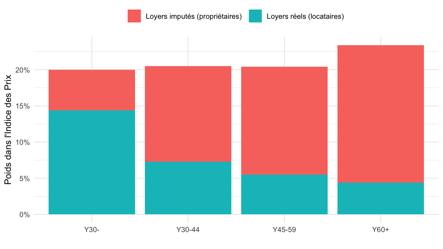
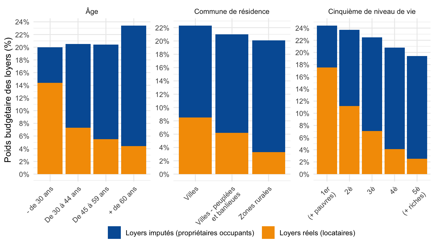
deg_urb <- read_parquet("deg_urb_fr.parquet")
data <- hbs_str_t225 |>
  rename(category = age) |>
  mutate(type = "age") |>
  bind_rows(hbs_str_t223 |>
              rename(category = quantile) |>
              mutate(type = "quantile")) |>
  bind_rows(hbs_str_t226 |>
              rename(category = deg_urb) |>
              mutate(type = "deg_urb")) |>
  filter(coicop %in% c("CP041", "CP042"),
         time == "2020",
         geo == "FR") %>%
  select_if(~ n_distinct(.) > 1) %>%
  select(type, everything(.)) |>
  arrange(coicop)

data |>
  spread(coicop, values) |>
  mutate(CP041_042 = CP041 + CP042) |>
print_table_conditional()| type | category | Age | Coicop | Quant_inc | Deg_urb | CP041 | CP042 | CP041_042 |
|---|---|---|---|---|---|---|---|---|
| age | Y_GE60 | 60 years or over | Actual rentals for housing | NA | NA | 44 | NA | NA |
| age | Y_GE60 | 60 years or over | Imputed rentals for housing | NA | NA | NA | 190 | NA |
| age | Y_LT30 | Less than 30 years | Actual rentals for housing | NA | NA | 144 | NA | NA |
| age | Y_LT30 | Less than 30 years | Imputed rentals for housing | NA | NA | NA | 56 | NA |
| age | Y30-44 | From 30 to 44 years | Actual rentals for housing | NA | NA | 73 | NA | NA |
| age | Y30-44 | From 30 to 44 years | Imputed rentals for housing | NA | NA | NA | 132 | NA |
| age | Y45-59 | From 45 to 59 years | Actual rentals for housing | NA | NA | 55 | NA | NA |
| age | Y45-59 | From 45 to 59 years | Imputed rentals for housing | NA | NA | NA | 149 | NA |
| deg_urb | DEG1 | NA | Actual rentals for housing | NA | Cities | 85 | NA | NA |
| deg_urb | DEG1 | NA | Imputed rentals for housing | NA | Cities | NA | 138 | NA |
| deg_urb | DEG2 | NA | Actual rentals for housing | NA | Towns and suburbs | 62 | NA | NA |
| deg_urb | DEG2 | NA | Imputed rentals for housing | NA | Towns and suburbs | NA | 148 | NA |
| deg_urb | DEG3 | NA | Actual rentals for housing | NA | Rural areas | 33 | NA | NA |
| deg_urb | DEG3 | NA | Imputed rentals for housing | NA | Rural areas | NA | 168 | NA |
| quantile | QU1 | NA | Actual rentals for housing | First quintile | NA | 175 | NA | NA |
| quantile | QU1 | NA | Imputed rentals for housing | First quintile | NA | NA | 69 | NA |
| quantile | QU2 | NA | Actual rentals for housing | Second quintile | NA | 112 | NA | NA |
| quantile | QU2 | NA | Imputed rentals for housing | Second quintile | NA | NA | 125 | NA |
| quantile | QU3 | NA | Actual rentals for housing | Third quintile | NA | 71 | NA | NA |
| quantile | QU3 | NA | Imputed rentals for housing | Third quintile | NA | NA | 154 | NA |
| quantile | QU4 | NA | Actual rentals for housing | Fourth quintile | NA | 41 | NA | NA |
| quantile | QU4 | NA | Imputed rentals for housing | Fourth quintile | NA | NA | 167 | NA |
| quantile | QU5 | NA | Actual rentals for housing | Fifth quintile | NA | 25 | NA | NA |
| quantile | QU5 | NA | Imputed rentals for housing | Fifth quintile | NA | NA | 169 | NA |
data_1 <- data |>
  mutate(Coicop = factor(coicop, levels = c("CP042", "CP041"), labels = c("Loyers imputés (propriétaires occupants)", "Loyers réels (locataires)")),
         Category = factor(category, levels = c("Y_LT30", "Y30-44", "Y45-59", "Y_GE60",
                                                "DEG1", "DEG2", "DEG3",
                                                "QUINTILE1", "QUINTILE2", "QUINTILE3", "QUINTILE4", "QUINTILE5"),
                           labels = c("- de 30 ans", "De 30 à 44 ans", "De 45 à 59 ans", "+ de 60 ans",
                                      "Villes", "Villes - peuplées\net banlieues", "Zones rurales",
                                      "1er\n(+ pauvres)", "2è", "3è", "4è", "5è\n(+ riches)")),
         Type = factor(type, levels = c("age", "deg_urb", "quantile"),
                       labels = c("Âge", "Commune de résidence", "Cinquième de niveau de vie"))) |>
  arrange(Coicop) |>
  mutate(values = values/1000) |>
  select(type, Type, category, Category, coicop, Coicop, values)
write.csv(data_1, file = "~/Desktop/graphique5.csv")

data_1 |>
  ggplot() + geom_col(aes(x = Category, y = values, fill = Coicop)) +
  theme_minimal() +
  xlab("") + ylab("Poids budgétaire des loyers (%)") +
  scale_y_continuous(breaks = 0.01*seq(-30, 50, 2),
                     labels = percent_format(accuracy = 1)) +
  theme(legend.position = "bottom",
        legend.title = element_blank(),
        legend.margin=margin(t=-35),
        axis.text.x = element_text(angle = 45, vjust = 1, hjust = 1)) +
  scale_fill_manual(values = c("#005DA4", "#F59C00")) +
  facet_wrap(~ Type, scales = "free")