Structure of consumption expenditure by age of the reference person and COICOP consumption purpose

Data - Eurostat

Info

Last observation: Annual: 2020 (N = 10,257)

First observation: Annual: 1988 (N = 3,440)

Last data update: 23 jul 2026, 23:06. Last compile: 24 jul 2026, 01:49

Structure

freq

hhcomp

coicop

unit

geo

Budget Shares Over Time: France, Two-Adult Households

hbs_str_t224 %>%
  filter(geo == "FR",
         hhcomp == "A2",
         coicop %in% c("CP01", "CP04", "CP07")) %>%
  year_to_date %>%
  mutate(values = values/1000) %>%
  ggplot + geom_line(aes(x = date, y = values, color = Coicop)) +
  theme_minimal() +
  scale_x_date(breaks = as.Date(paste0(seq(1985, 2100, 5), "-01-01")),
               labels = date_format("%Y")) +
  theme(legend.position = "bottom",
        legend.title = element_blank()) +
  guides(color = guide_legend(nrow = 3)) +
  xlab("") + ylab("Share of household budget") +
  scale_y_continuous(labels = scales::percent_format(accuracy = 1))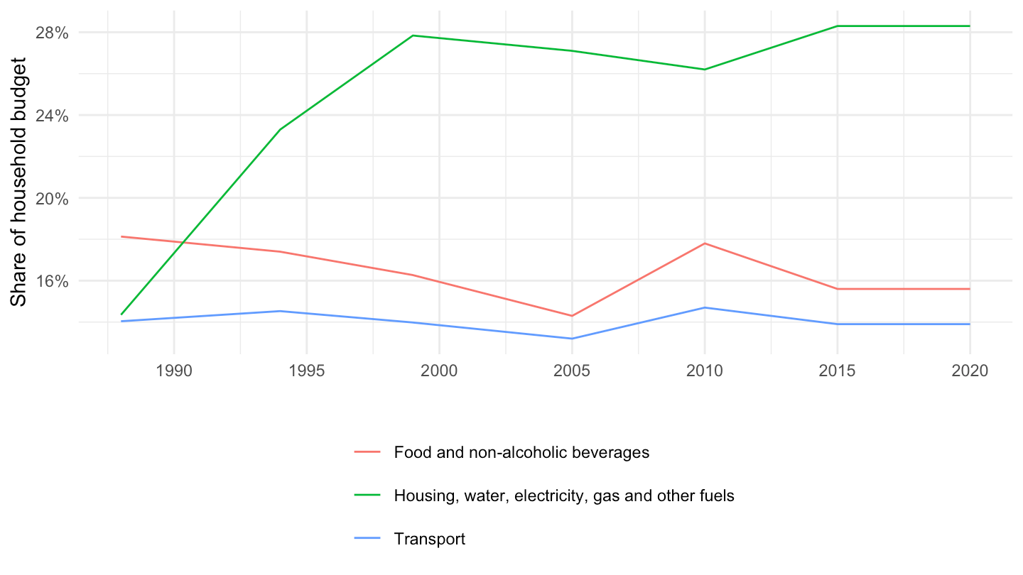

Food vs. Housing Budget Shares, 2020

France, Germany, Italy, Spain

hbs_str_t224 %>%
  filter(time == "2020",
         hhcomp == "A2",
         coicop %in% c("CP01", "CP04"),
         geo %in% c("FR", "DE", "IT", "ES")) %>%
  mutate(values = values/1000) %>%
  ggplot + geom_col(aes(x = Geo, y = values, fill = Coicop), position = "dodge") +
  theme_minimal() +
  theme(legend.title = element_blank()) +
  xlab("") + ylab("Share of household budget") +
  scale_y_continuous(labels = scales::percent_format(accuracy = 1))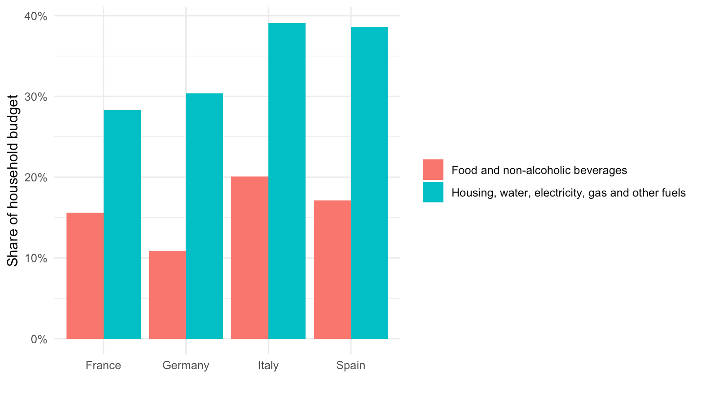

coicop

France - Compare

2020, HBS

hbs_str_t224 %>%
  filter(time == "2020",
         geo == "FR") %>%
  
  select_if(~ n_distinct(.) > 1) %>%
  spread(hhcomp, values) %>%
  select_if(~ n_distinct(.) > 1) %>%
  print_table_conditional

2015, HBS

All

hbs_str_t224 %>%
  filter(time == "2015",
         geo == "FR") %>%
  
  select_if(~ n_distinct(.) > 1) %>%
  spread(hhcomp, values) %>%
  select_if(~ n_distinct(.) > 1) %>%
  print_table_conditional

2-digit

hbs_str_t224 %>%
  filter(time == "2015",
         geo == "FR",
         nchar(coicop) == 4) %>%
  
  select_if(~ n_distinct(.) > 1) %>%
  spread(hhcomp, values) %>%
  select_if(~ n_distinct(.) > 1) %>%
  print_table_conditional

All quintiles

Sums

2-digit

hbs_str_t224 %>%
  filter(time == "2020",
         substr(coicop, 1, 2) == "CP",
         nchar(coicop) == 4) %>%
  
  select_if(~ n_distinct(.) > 1) %>%
  group_by(hhcomp, geo, Geo) %>%
  summarise(values = sum(values)) %>%
  spread(hhcomp, values) %>%
  print_table_conditional

3-digit

hbs_str_t224 %>%
  filter(time == "2020",
         substr(coicop, 1, 2) == "CP",
         nchar(coicop) == 5) %>%
  
  select_if(~ n_distinct(.) > 1) %>%
  group_by(hhcomp, geo, Geo) %>%
  summarise(values = sum(values)) %>%
  spread(hhcomp, values) %>%
  print_table_conditional

geo	Geo	A_GE3	A_GE3_DCH	A1	A1_DCH	A2	A2_DCH	UNK
AT	Austria	1001	999	998	999	997	1000	NA
BE	Belgium	1000	1001	997	999	1000	997	NA
BG	Bulgaria	998	999	998	997	1000	1003	NA
CY	Cyprus	996	997	1001	996	997	993	NA
CZ	Czechia	1002	1003	999	997	998	997	NA
DE	Germany	984	986	994	990	990	992	NA
DK	Denmark	1000	997	999	1001	1004	1002	NA
EE	Estonia	990	996	976	983	986	991	NA
EL	Greece	1004	999	1001	1000	997	1002	NA
ES	Spain	1001	1003	998	1001	1001	995	NA
FI	Finland	984	983	982	974	979	976	NA
FR	France	994	987	992	994	989	986	NA
HR	Croatia	999	997	998	1004	994	1001	NA
HU	Hungary	1000	1001	1000	998	999	999	NA
IE	Ireland	999	1001	999	1000	1000	999	NA
IT	Italy	1002	1000	1001	997	998	1001	NA
LT	Lithuania	998	999	997	999	1000	998	NA
LU	Luxembourg	1003	997	1000	1000	999	999	NA
LV	Latvia	1000	997	1000	998	998	998	NA
ME	Montenegro	983	982	987	991	980	984	NA
MT	Malta	998	999	996	999	1001	1001	NA
NL	Netherlands	1001	997	1000	1001	1000	1001	NA
NO	Norway	986	999	993	993	994	997	NA
PL	Poland	998	1000	1001	999	999	1000	NA
RS	Serbia	1000	1000	997	1002	999	999	NA
SI	Slovenia	998	1000	1000	1003	997	1001	NA
SK	Slovakia	1000	998	1002	997	995	996	NA
TR	Türkiye	1000	999	1002	1001	1000	999	NA

CP041, CP042, CP041_042

2015

France

hbs_str_t224 %>%
  filter(coicop %in% c("CP041", "CP042"),
         time == "2015",
         geo %in% c("FR")) %>%
  spread(coicop, values) %>%
  mutate(CP041_042 = CP041 + CP042) %>%
  gather(coicop, values, CP041, CP042, CP041_042) %>%
  
  
  left_join(colors, by = c("Geo" = "country")) %>%
  mutate(Coicop = ifelse(coicop == "CP041_042", "Imputed rentals plus actual rentals", Coicop),
         hhcomp = ifelse(hhcomp == "Y_GE60", "Y60+", hhcomp),
         hhcomp = ifelse(hhcomp == "Y_LT30", "Y30-", hhcomp)) %>%
  ggplot + geom_line(aes(x = hhcomp, y = values/1000, color = Coicop, group = Coicop)) +
  theme_minimal() +
  xlab("") + ylab("Weight in CPI") +
  scale_y_continuous(breaks = 0.01*seq(-30, 50, 2),
                     labels = percent_format(accuracy = 1)) +
  theme(legend.position = c(0.2, 0.9),
        legend.title = element_blank())