Last observation: Q: 2024-09-30 (N = 4) · A: 2023-12-31 (N = 50)
First observation: A: 1995-12-31 (N = 2) · Q: 1995-12-31 (N = 1)
Last data update: 10 août 2026, 16:21. Last compile: 30 août 2026, 10:25
 Data - Banque de France
Last observation: Q: 2024-09-30 (N = 4) · A: 2023-12-31 (N = 50)
First observation: A: 1995-12-31 (N = 2) · Q: 1995-12-31 (N = 1)
Last data update: 10 août 2026, 16:21. Last compile: 30 août 2026, 10:25
Households’ financial saving and wealth, Financial accounts of non-financial agents, 15 April 2024, 2023Q4. pdf html
Households’ financial saving and wealth, 2023Q3. pdf
Households’ financial saving and wealth, 2023Q2. pdf
Quarterly presentation of household saving, 2023Q1. html pdf
Methodology. pdf
List of series. html
Households’ financial saving and wealth, 2022Q2. pdf
Household saving, 2021Q1. pdf
Debt ratio of non-financial agents – International comparisons, 2020Q4. html / pdf
Household saving, 2020Q3. pdf
CFT |>


  group_by(INSTR_ASSET, Instr_asset) |>
  summarise(Nobs = n()) |>
  #arrange(-Nobs) %>%
print_table_conditional()ig_b("bdf", "CFT-2024T2")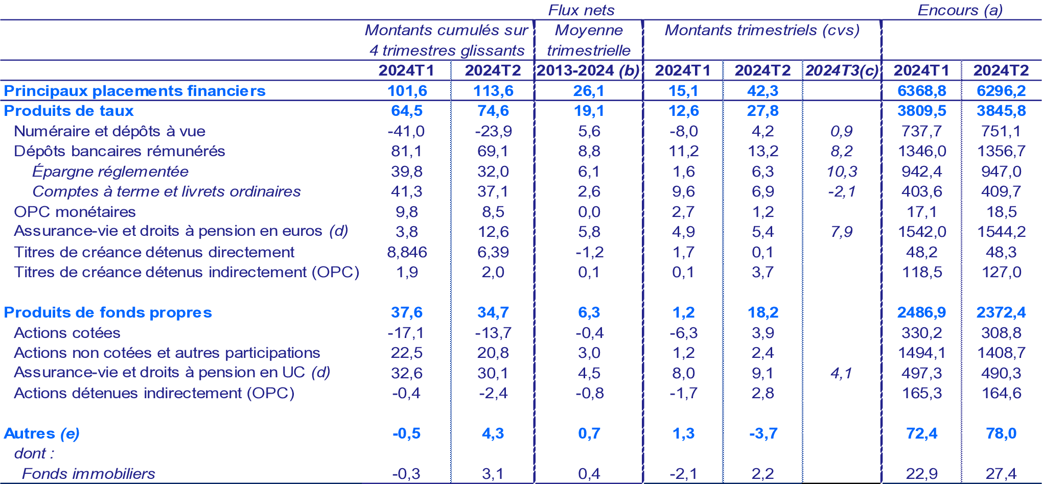
ig_b("bdf", "CFT-2023T4")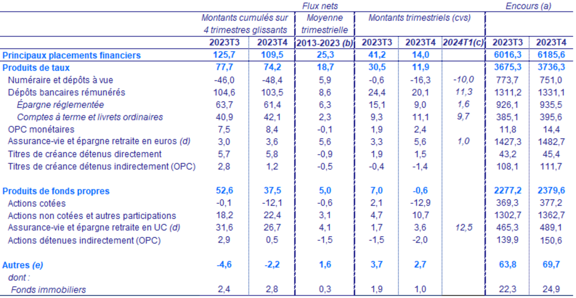
CFT |>

  filter(STO == "LE",
         INSTR_ASSET %in% c("PDTX")) |>
  na.omit() |>
  ggplot() + geom_line(aes(x = date, y = value, color = Variable)) +
  xlab("") + ylab("") + theme_minimal() +
  scale_x_date(breaks = "1 year",
               labels = date_format("%Y")) +
  scale_y_log10(breaks = seq(-200, 10000, 100),
                     labels = dollar_format(acc = 1, prefix = "", su = "Mds€")) +
  theme(legend.position = c(0.35, 0.9),
        legend.title = element_blank(),
        legend.direction = "vertical") +
  geom_label(data = . %>% filter(date == as.Date("2023-12-31")),
             aes(x = date, y = value, color = Variable, label = round(value)))
CFT |>

  filter(STO == "LE",
         INSTR_ASSET %in% c("PDFP")) |>
  na.omit() |>
  ggplot() + geom_line(aes(x = date, y = value, color = Variable)) +
  xlab("") + ylab("") + theme_minimal() +
  scale_x_date(breaks = "1 year",
               labels = date_format("%Y")) +
  scale_y_log10(breaks = seq(-200, 10000, 100),
                     labels = dollar_format(acc = 1, prefix = "", su = "Mds€")) +
  theme(legend.position = c(0.35, 0.9),
        legend.title = element_blank(),
        legend.direction = "vertical") +
  geom_label(data = . %>% filter(date == as.Date("2023-12-31")),
             aes(x = date, y = value, color = Variable, label = round(value)))
CFT |>

  filter(STO == "LE",
         INSTR_ASSET %in% c("PDFP", "F51", "F511", "F51M", "F52")) |>
  na.omit() |>
  ggplot() + geom_line(aes(x = date, y = value, color = Variable)) +
  xlab("") + ylab("") + theme_minimal() +
  scale_x_date(breaks = "1 year",
               labels = date_format("%Y")) +
  scale_y_log10(breaks = seq(-200, 10000, 100),
                     labels = dollar_format(acc = 1, prefix = "", su = "Mds€")) +
  theme(legend.position = c(0.5, 0.7),
        legend.title = element_blank(),
        legend.direction = "vertical") +
  geom_label(data = . %>% filter(date == as.Date("2023-12-31")),
             aes(x = date, y = value, color = Variable, label = round(value)))
CFT |>

  filter(STO == "LE",
         INSTR_ASSET %in% c("F62A", "F62B", "F29R", "F2A", "F29Z")) |>
  na.omit() |>
  ggplot() + geom_line(aes(x = date, y = value, color = Variable)) +
  xlab("") + ylab("") + theme_minimal() +
  scale_x_date(breaks = "1 year",
               labels = date_format("%Y")) +
  scale_y_continuous(breaks = seq(-200, 10000, 100),
                     labels = dollar_format(acc = 1, prefix = "", su = "Mds€")) +
  theme(legend.position = c(0.45, 0.17),
        legend.title = element_blank(),
        legend.direction = "vertical") +
  geom_label(data = . %>% filter(date == as.Date("2023-12-31")),
             aes(x = date, y = value, color = Variable, label = round(value)))
CFT |>

  filter(STO == "LE",
         INSTR_ASSET %in% c("F62A", "F62B", "F29R", "F2A", "F29Z")) |>
  na.omit() |>
  ggplot() + geom_line(aes(x = date, y = value, color = Variable)) +
  xlab("") + ylab("") + theme_minimal() +
  scale_x_date(breaks = "1 year",
               labels = date_format("%Y")) +
  scale_y_log10(breaks = seq(-200, 10000, 100),
                     labels = dollar_format(acc = 1, prefix = "", su = "Mds€")) +
  theme(legend.position = c(0.45, 0.17),
        legend.title = element_blank(),
        legend.direction = "vertical") +
  geom_label(data = . %>% filter(date == as.Date("2023-12-31")),
             aes(x = date, y = value, color = Variable, label = round(value)))
CFT |>


  filter(REF_AREA %in% c("FR", "IT", "DE"),
         INSTR_ASSET == "F2A",
         STO == "LE") |>
  mutate(Ref_area = ifelse(REF_AREA == "I8", "Europe", Ref_area)) |>
  left_join(colors, by = c("Ref_area" = "country")) |>
  na.omit() |>
  ggplot() + geom_line(aes(x = date, y = value, color = color)) +
  xlab("") + ylab("") + theme_minimal() + scale_color_identity() + add_3flags +
  scale_x_date(breaks = "1 year",
               labels = date_format("%Y")) +
  scale_y_log10(breaks = seq(100, 4000, 100),
                labels = dollar_format(accuracy = 1, pre = "", su = " Mds€")) +
  geom_label(data = . %>% filter(date == as.Date("2023-12-31")),
             aes(x = date, y = value, label = round(value)))
CFT |>


  filter(REF_AREA %in% c("FR"),
         INSTR_ASSET %in% c("F2A", "F29Z", "F62B", "F29R"),
         STO == "LE") |>
  select(date, value, Instr_asset) |>
  na.omit() |>
  ggplot() + geom_line(aes(x = date, y = value, color = Instr_asset)) +
  xlab("") + ylab("") + theme_minimal() +

  scale_x_date(breaks = "1 year",
               labels = date_format("%Y")) +
  scale_y_log10(breaks = seq(100, 4000, 100),
                labels = dollar_format(accuracy = 1, pre = "", su = " Mds€")) +
  theme(legend.position = c(0.4, 0.4),
        legend.title = element_blank(),
        legend.direction = "vertical") +
  geom_label(data = . %>% filter(date == as.Date("2023-12-31")),
             aes(x = date, y = value, color = Instr_asset, label = round(value)))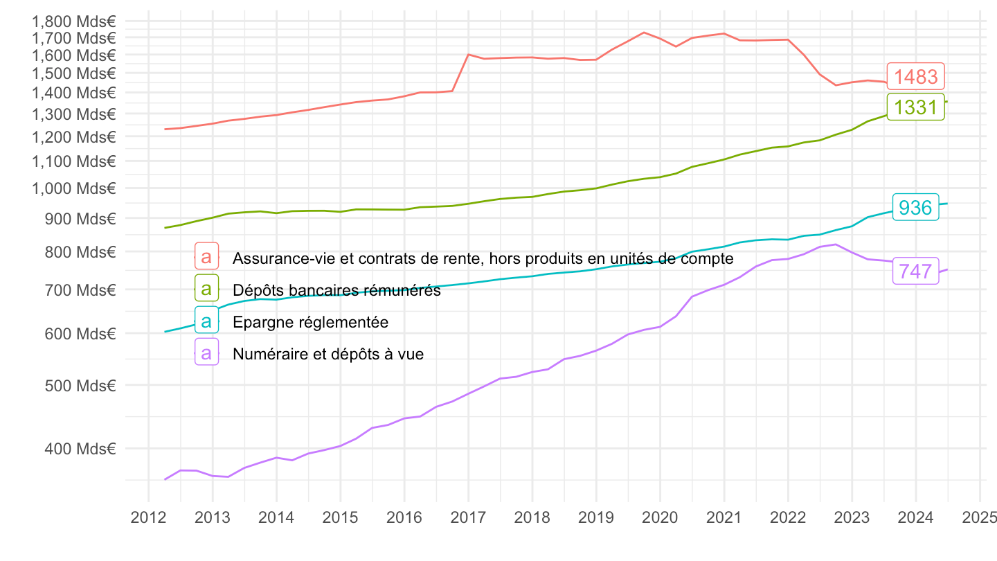
CFT |>


  filter(REF_AREA %in% c("FR"),
         INSTR_ASSET %in% c("F2A", "F29Z", "F62B"),
         STO == "LE") |>
  select(date, value, Instr_asset) |>
  na.omit() |>
  ggplot() + geom_line(aes(x = date, y = value, color = Instr_asset)) +
  xlab("") + ylab("") + theme_minimal() +

  scale_x_date(breaks = "1 year",
               labels = date_format("%Y")) +
  scale_y_log10(breaks = seq(100, 4000, 100),
                labels = dollar_format(accuracy = 1, pre = "", su = " Mds€")) +
  theme(legend.position = c(0.4, 0.4),
        legend.title = element_blank(),
        legend.direction = "vertical") +
  geom_label(data = . %>% filter(date == as.Date("2023-12-31")),
             aes(x = date, y = value, color = Instr_asset, label = round(value)))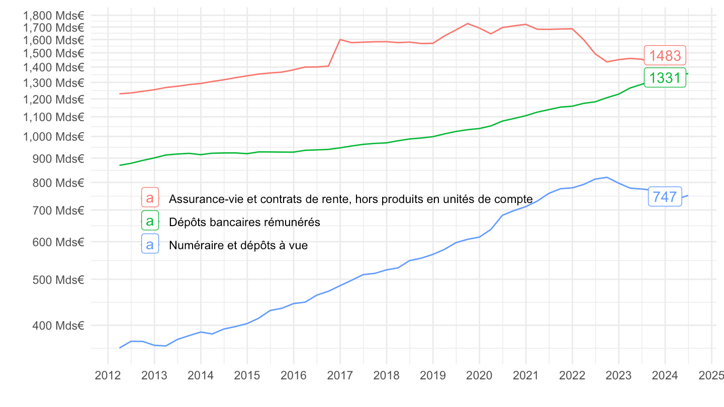
CFT |>


  filter(REF_AREA %in% c("FR"),
         INSTR_ASSET %in% c("F2A", "F29Z", "F62B"),
         STO == "LE") |>
  select(date, value, Instr_asset) |>
  na.omit() |>
  filter(date >= as.Date("2022-01-01")) |>
  ggplot() + geom_line(aes(x = date, y = value, color = Instr_asset)) +
  xlab("") + ylab("") + theme_minimal() +

  scale_x_date(breaks = "3 months",
               labels = date_format("%b %Y")) +
  scale_y_log10(breaks = seq(100, 4000, 100),
                labels = dollar_format(accuracy = 1, pre = "", su = " Mds€")) +
  theme(legend.position = c(0.4, 0.4),
        legend.title = element_blank(),
        legend.direction = "vertical") +
  geom_label(data = . %>% filter(date == as.Date("2023-12-31")),
             aes(x = date, y = value, color = Instr_asset, label = round(value)))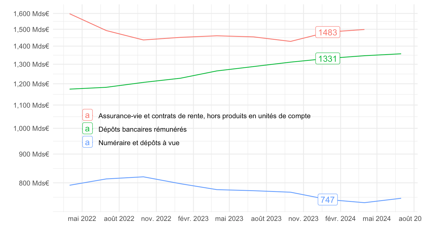
CFT |>


  filter(REF_AREA %in% c("FR"),
         INSTR_ASSET %in% c("F2A", "F29Z", "F62B", "F29R"),
         STO == "F",
         TRANSFORMATION == "C4") |>
  #filter(date >= as.Date("2016-01-01")) %>%
  select(date, value, Instr_asset) |>
  na.omit() |>
  ggplot() + geom_line(aes(x = date, y = value, color = Instr_asset)) +
  xlab("") + ylab("") + theme_minimal() +

  scale_x_date(breaks = "1 year",
               labels = date_format("%Y")) +
  scale_y_continuous(breaks = seq(-2000, 4000, 10),
                labels = dollar_format(accuracy = 1, pre = "", su = " Mds€")) +
  theme(legend.position = c(0.4, 0.8),
        legend.title = element_blank(),
        legend.direction = "vertical")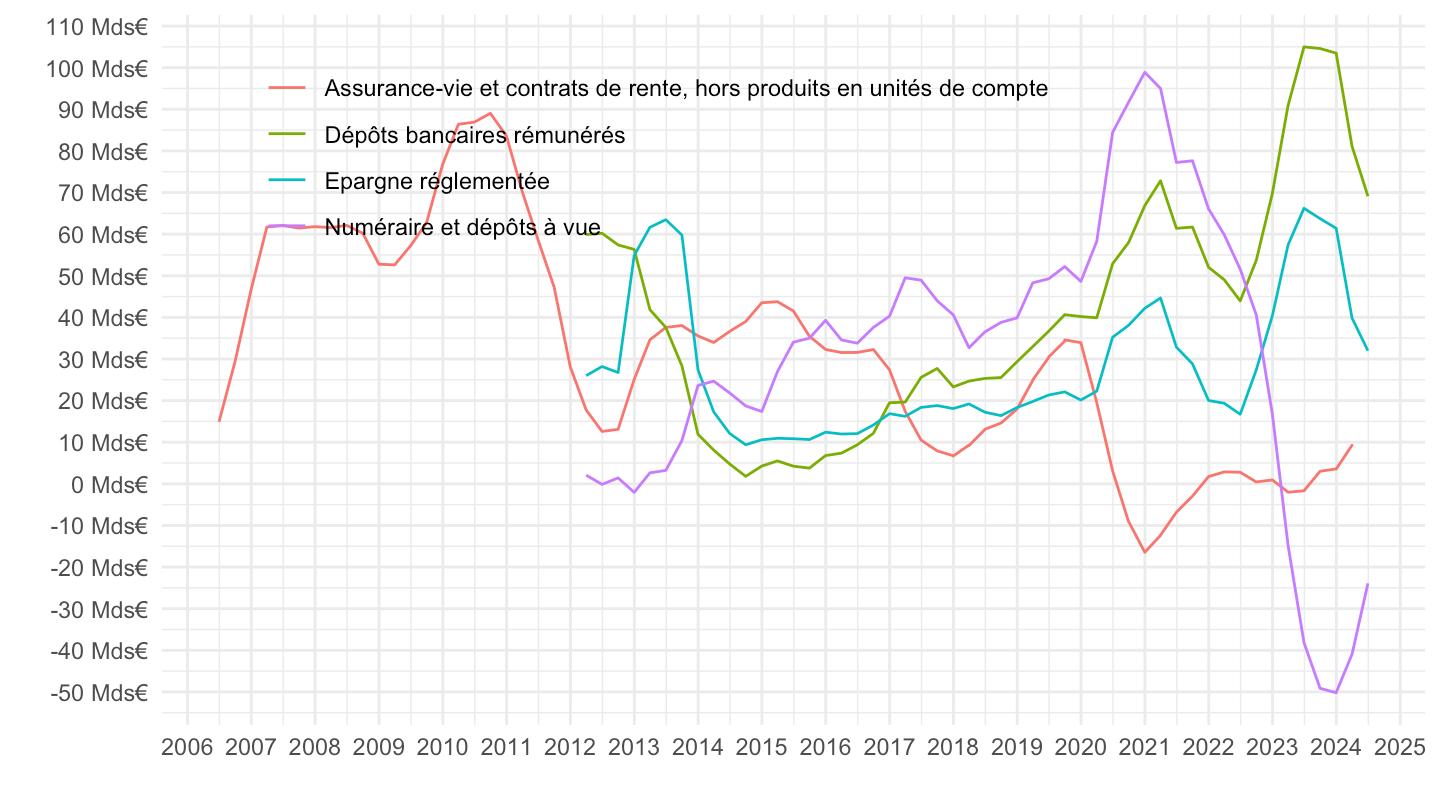
CFT |>


  filter(REF_AREA %in% c("FR"),
         INSTR_ASSET %in% c("F2A", "F29Z", "F62B", "F29R"),
         STO == "F",
         TRANSFORMATION == "N",
         FREQ == "Q") |>
  filter(date >= as.Date("2010-01-01")) |>
  ggplot() + geom_line(aes(x = date, y = value, color = Instr_asset)) +
  xlab("") + ylab("") + theme_minimal() +

  scale_x_date(breaks = "1 year",
               labels = date_format("%Y")) +
  scale_y_continuous(breaks = seq(-1000, 4000, 10),
                labels = dollar_format(accuracy = 1, pre = "", su = " Mds€")) +
  theme(legend.position = c(0.4, 0.8),
        legend.title = element_blank(),
        legend.direction = "vertical")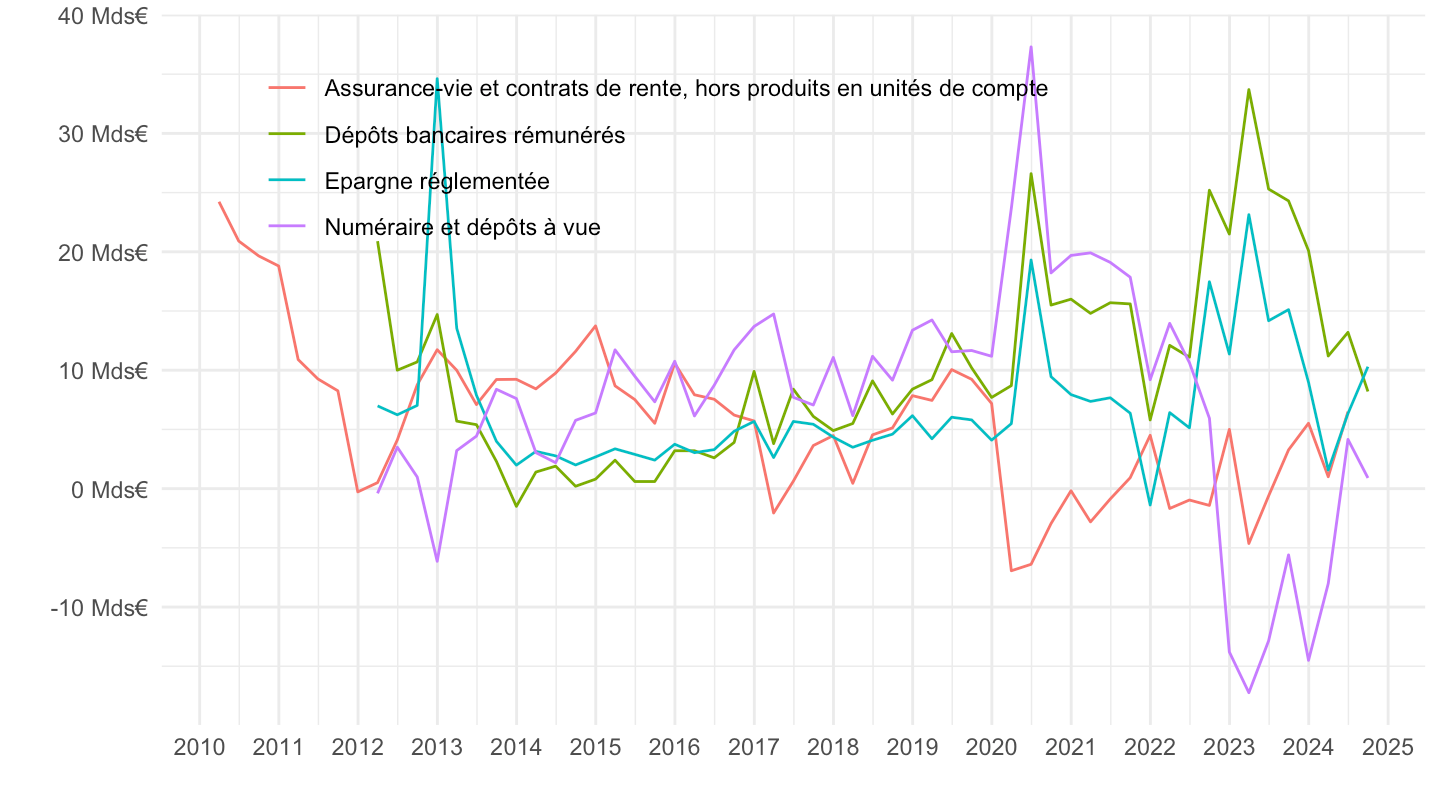
CFT |>


  filter(REF_AREA %in% c("FR"),
         INSTR_ASSET %in% c("F2A", "F29Z", "F62B", "F29R"),
         STO == "F",
         TRANSFORMATION == "N",
         FREQ == "Q") |>
  filter(date >= as.Date("2016-01-01")) |>
  ggplot() + geom_line(aes(x = date, y = value, color = Instr_asset)) +
  xlab("") + ylab("") + theme_minimal() +

  scale_x_date(breaks = "1 year",
               labels = date_format("%Y")) +
  scale_y_continuous(breaks = seq(-1000, 4000, 10),
                labels = dollar_format(accuracy = 1, pre = "", su = " Mds€")) +
  theme(legend.position = c(0.4, 0.9),
        legend.title = element_blank(),
        legend.direction = "vertical") +
  geom_hline(yintercept = 0, linetype = "dashed")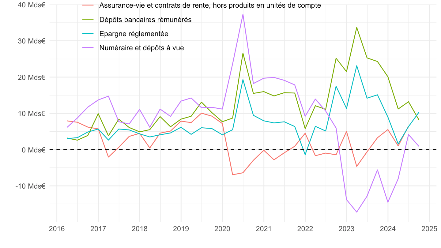
CFT |>


  filter(REF_AREA %in% c("FR"),
         INSTR_ASSET %in% c( "F511", "F51M", "F51"),
         STO == "LE") |>
  na.omit() |>
  ggplot() + geom_line(aes(x = date, y = value, color = Instr_asset)) +
  xlab("") + ylab("") + theme_minimal() +

  scale_x_date(breaks = "1 year",
               labels = date_format("%Y")) +
  scale_y_log10(breaks = seq(100, 4000, 100),
                labels = dollar_format(accuracy = 1, pre = "", su = " Mds€")) +
  theme(legend.position = c(0.4, 0.6),
        legend.title = element_blank(),
        legend.direction = "vertical") +
  geom_label(data = . %>% filter(date == as.Date("2023-12-31")),
             aes(x = date, y = value, color = Instr_asset, label = round(value)))
CFT |>


  filter(REF_AREA %in% c("FR"),
         INSTR_ASSET %in% c( "F511", "F51M", "F62A"),
         STO == "LE") |>
  na.omit() |>
  ggplot() + geom_line(aes(x = date, y = value, color = Instr_asset)) +
  xlab("") + ylab("") + theme_minimal() +

  scale_x_date(breaks = "1 year",
               labels = date_format("%Y")) +
  scale_y_log10(breaks = seq(100, 4000, 100),
                labels = dollar_format(accuracy = 1, pre = "", su = " Mds€")) +
  theme(legend.position = c(0.4, 0.6),
        legend.title = element_blank(),
        legend.direction = "vertical") +
  geom_label(data = . %>% filter(date == as.Date("2023-12-31")),
             aes(x = date, y = value, color = Instr_asset, label = round(value)))
CFT |>


  filter(REF_AREA %in% c("FR"),
         INSTR_ASSET %in% c( "F511", "F51M", "F62A"),
         STO == "F",
         TRANSFORMATION == "N",
         FREQ == "Q") |>
  filter(date >= as.Date("2016-01-01")) |>
  ggplot() + geom_line(aes(x = date, y = value, color = Instr_asset)) +
  xlab("") + ylab("") + theme_minimal() +

  scale_x_date(breaks = "1 year",
               labels = date_format("%Y")) +
  scale_y_continuous(breaks = seq(-2000, 4000, 5),
                labels = dollar_format(accuracy = 1, pre = "", su = " Mds€")) +
  theme(legend.position = c(0.4, 0.4),
        legend.title = element_blank(),
        legend.direction = "vertical")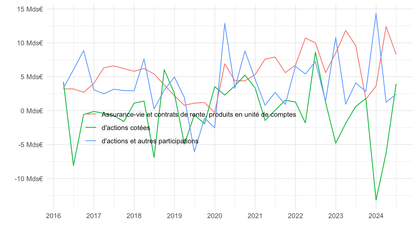
CFT |>


  filter(REF_AREA %in% c("FR"),
         INSTR_ASSET %in% c("F2A", "F29Z"),
         STO == "LE") |>
  na.omit() |>
  ggplot() + geom_line(aes(x = date, y = value, color = Instr_asset)) +
  xlab("") + ylab("") + theme_minimal() +

  scale_x_date(breaks = "1 year",
               labels = date_format("%Y")) +
  scale_y_log10(breaks = seq(100, 4000, 100),
                labels = dollar_format(accuracy = 1, pre = "", su = " Mds€")) +
  theme(legend.position = c(0.75, 0.1),
        legend.title = element_blank(),
        legend.direction = "vertical") +
  geom_label(data = . %>% filter(date == as.Date("2023-12-31")),
             aes(x = date, y = value, color = Instr_asset, label = round(value)))
CFT |>

  filter(variable %in% c("CFT.Q.S.FR.W0.S1M.S1.N.A.F.F62B._Z._Z.XDC._T.S.V.N._T",
                         "CFT.Q.S.FR.W0.S1M.S1.N.A.F.F62A._Z._Z.XDC._T.S.V.N._T",
                         "CFT.Q.S.FR.W0.S1M.S1.N.A.F.F29R.T._Z.XDC._T.S.V.N._T",
                         "CFT.Q.S.FR.W0.S1M.S1.N.A.F.F2A.T._Z.XDC._T.S.V.N._T")) |>
  na.omit() |>
  ggplot() + geom_line(aes(x = date, y = value, color = Variable)) +
  xlab("") + ylab("") + theme_minimal() +

  scale_x_date(breaks = "1 year",
               labels = date_format("%Y")) +
  scale_y_continuous(breaks = seq(-200, 1000, 5),
                     limits = c(-25 ,40),
                     labels = dollar_format(acc = 1, prefix = "", su = "Mds€")) +
  theme(legend.position = c(0.45, 0.17),
        legend.title = element_blank(),
        legend.direction = "vertical")
CFT |>

  filter(variable %in% c("CFT.Q.S.FR.W0.S1M.S1.N.A.F.F62B._Z._Z.XDC._T.S.V.N._T",
                         "CFT.Q.S.FR.W0.S1M.S1.N.A.F.F29Z.T._Z.XDC._T.S.V.N._T",
                         "CFT.Q.S.FR.W0.S1M.S1.N.A.F.F29R.T._Z.XDC._T.S.V.N._T",
                         "CFT.Q.S.FR.W0.S1M.S1.N.A.F.F2A.T._Z.XDC._T.S.V.N._T")) |>
  filter(date >= as.Date("2015-01-01")) |>
  ggplot() + geom_line(aes(x = date, y = value, color = Variable)) +
  xlab("") + ylab("") + theme_minimal() +

  scale_x_date(breaks = "1 year",
               labels = date_format("%Y")) +
  scale_y_continuous(breaks = seq(-200, 1000, 5),
                     limits = c(-5 ,40),
                     labels = dollar_format(acc = 1, prefix = "", su = "Mds€")) +
  theme(legend.position = c(0.45, 0.8),
        legend.title = element_blank(),
        legend.direction = "vertical")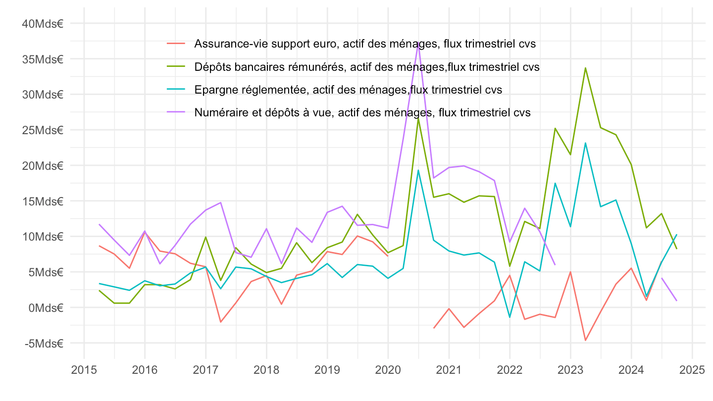
The household saving rate is the ratio of households’ gross saving (B8G) to gross disposable income adjusted for changes in pension entitlements. Gross disposable income (B6G) corresponds to the income received by households (earned income and property income) after redistribution operations (adding cash social benefits received, subtracting contributions and taxes).
As for the financial saving rate, it is the share of gross disposable income invested in financial assets.
the saving rate is obtained by dividing gross saving by gross disposable income adjusted for the change in households’ entitlements under pension funds, with both series previously seasonally adjusted
the financial saving rate is estimated by subtracting gross fixed capital formation from gross saving, then dividing the result by gross disposable income adjusted for the change in households’ entitlements under pension funds, and then seasonally adjusting the result.
CFT |>

  filter(variable %in% c("CFT.A.N.FR.W0.S1M.S1.N.B.B8G._Z._Z._Z.XDC_R_B6G_S1M._T.S.V.N._T",
                         "CFT.A.N.FR.W0.S1M.S1.N.B.B9Z._Z._Z._Z.XDC_R_B6G_S1M._T.S.V.N._T")) |>
  na.omit() |>
  ggplot() + geom_line(aes(x = date, y = value/100, color = Variable)) +
  xlab("") + ylab("") + theme_minimal() +

  scale_x_date(breaks = "1 year",
               labels = date_format("%Y")) +
  scale_y_continuous(breaks = 0.01*seq(-10, 100, 1),
                labels = percent_format(accuracy = 1)) +
  theme(legend.position = c(0.4, 0.9),
        legend.title = element_blank(),
        legend.direction = "vertical")
CFT |>

  filter(variable %in% c("CFT.Q.N.FR.W0.S1M.S1.N.B.B8G._Z._Z._Z.XDC_R_B6G_S1M._T.S.V.C4._T",
                         "CFT.Q.N.FR.W0.S1M.S1.N.B.B9Z._Z._Z._Z.XDC_R_B6G_S1M._T.S.V.C4._T")) |>
  na.omit() |>
  ggplot() + geom_line(aes(x = date, y = value/100, color = Variable)) +
  xlab("") + ylab("") + theme_minimal() +
  scale_x_date(breaks = "2 years",
               labels = date_format("%Y")) +
  scale_y_continuous(breaks = 0.01*seq(-10, 100, 1),
                labels = percent_format(accuracy = 1)) +
  theme(legend.position = c(0.42, 0.9),
        legend.title = element_blank(),
        legend.direction = "vertical")
CFT |>

  filter(variable %in% c("CFT.Q.N.FR.W0.S1M.S1.N.B.B8G._Z._Z._Z.XDC_R_B6G_S1M._T.S.V.C4._T",
                         "CFT.Q.N.FR.W0.S1M.S1.N.B.B9Z._Z._Z._Z.XDC_R_B6G_S1M._T.S.V.C4._T")) |>
  na.omit() |>
  filter(date >= as.Date("2010-01-01")) |>
  ggplot() + geom_line(aes(x = date, y = value/100, color = Variable)) +
  xlab("") + ylab("") + theme_minimal() +
  scale_x_date(breaks = "2 years",
               labels = date_format("%Y")) +
  scale_y_continuous(breaks = 0.01*seq(-10, 100, 1),
                labels = percent_format(accuracy = 1)) +
  theme(legend.position = c(0.45, 0.9),
        legend.title = element_blank(),
        legend.direction = "vertical")
REF_AREA <- read_parquet("REF_AREA.parquet")
CFT |>


  filter(FREQ == "Q",
         UNIT_MEASURE == "XDC_R_B6G_S1M",
         REF_SECTOR == "S1M",
         date == as.Date("2020-01-01")) |>
  select(Variable, Ref_area, value) |>
  arrange(Ref_area) |>
print_table_conditional()| Variable | Ref_area | value |
|---|---|---|
| character(0) | c(":--------:", ":--------:", ":-----:") | character(0) |
CFT |>


  filter(FREQ == "Q",
         REF_AREA %in% c("FR", "IT", "DE"),
         UNIT_MEASURE == "XDC_R_B6G_S1M",
         STO == "B9Z",
         REF_SECTOR == "S1M") |>
  mutate(value = value/100) |>
  na.omit() |>
  ggplot() + geom_line(aes(x = date, y = value, color = Ref_area)) +
  xlab("") + ylab("") + theme_minimal() +
  scale_color_manual(values = c("#002395", "#000000", "#009246")) +
  scale_x_date(breaks = "2 years",
               labels = date_format("%Y")) +
  add_3flags +
  scale_y_continuous(breaks = 0.01*seq(-10, 100, 1),
                labels = percent_format(accuracy = 1)) +
  theme(legend.position = "none")
CFT |>


  filter(FREQ == "Q",
         UNIT_MEASURE == "XDC_R_B6G_S1M",
         STO == "B9Z",
         REF_SECTOR == "S1M") |>
  left_join(colors, by = c("Ref_area" = "country")) |>
  mutate(value = value/100) |>
  na.omit() |>
  ggplot() + geom_line(aes(x = date, y = value, color = color)) +
  xlab("") + ylab("") + theme_minimal() + scale_color_identity() + add_6flags +
  scale_x_date(breaks = "2 years",
               labels = date_format("%Y")) +
  scale_y_continuous(breaks = 0.01*seq(-10, 100, 1),
                labels = percent_format(accuracy = 1))
CFT |>


  filter(FREQ == "Q",
         UNIT_MEASURE == "XDC_R_B6G_S1M",
         STO == "B9Z",
         REF_SECTOR == "S1M") |>
  left_join(colors, by = c("Ref_area" = "country")) |>
  mutate(value = value/100) |>
  filter(date >= as.Date("2007-01-01")) |>
  na.omit() |>
  ggplot() + geom_line(aes(x = date, y = value, color = color)) +
  xlab("") + ylab("") + theme_minimal() + scale_color_identity() + add_6flags +
  scale_x_date(breaks = "1 year",
               labels = date_format("%Y")) +
  scale_y_continuous(breaks = 0.01*seq(-10, 100, 1),
                labels = percent_format(accuracy = 1))
CFT |>


  filter(FREQ == "Q",
         UNIT_MEASURE == "XDC_R_B6G_S1M",
         STO == "B9Z",
         REF_SECTOR == "S1M") |>
  left_join(colors, by = c("Ref_area" = "country")) |>
  mutate(value = value/100) |>
  filter(date >= as.Date("2015-01-01")) |>
  na.omit() |>
  ggplot() + geom_line(aes(x = date, y = value, color = color)) +
  xlab("") + ylab("Financial saving rate (%)") + theme_minimal() + scale_color_identity() + add_6flags +
  scale_x_date(breaks = "1 year",
               labels = date_format("%Y")) +
  scale_y_continuous(breaks = 0.01*seq(-10, 100, 1),
                labels = percent_format(accuracy = 1))
CFT |>


  filter(FREQ == "Q",
         REF_AREA %in% c("FR", "IT", "DE"),
         UNIT_MEASURE == "XDC_R_B6G_S1M",
         STO == "B8G",
         REF_SECTOR == "S1M") |>
  left_join(colors, by = c("Ref_area" = "country")) |>
  mutate(value = value/100) |>
  na.omit() |>
  ggplot() + geom_line(aes(x = date, y = value, color = color)) +
  xlab("") + ylab("") + theme_minimal() + scale_color_identity() + add_3flags +
  scale_x_date(breaks = "2 years",
               labels = date_format("%Y")) +
  scale_y_continuous(breaks = 0.01*seq(-10, 100, 1),
                labels = percent_format(accuracy = 1))
CFT |>


  filter(FREQ == "Q",
         UNIT_MEASURE == "XDC_R_B6G_S1M",
         STO == "B8G",
         REF_SECTOR == "S1M") |>
  left_join(colors, by = c("Ref_area" = "country")) |>
  mutate(value = value/100) |>
  na.omit() |>
  ggplot() + geom_line(aes(x = date, y = value, color = color)) +
  xlab("") + ylab("") + theme_minimal() + scale_color_identity() + add_6flags +
  scale_x_date(breaks = "2 years",
               labels = date_format("%Y")) +
  scale_y_continuous(breaks = 0.01*seq(-10, 100, 1),
                labels = percent_format(accuracy = 1))
CFT |>


  filter(INSTR_ASSET == "DETT",
         UNIT_MEASURE == "XDC_R_B1GQ_CY",
         REF_SECTOR == "S1M") |>
  mutate(Ref_area = ifelse(REF_AREA == "I8", "Europe", Ref_area)) |>
  mutate(Ref_area = ifelse(REF_AREA == "UK", "United Kingdom", Ref_area)) |>
  left_join(colors, by = c("Ref_area" = "country")) |>
  mutate(value = value/100) |>
  arrange(date) |>
  select(REF_AREA,everything()) |>
  ggplot() + geom_line(aes(x = date, y = value, color = color)) +
  xlab("") + ylab("") + theme_minimal() + scale_color_identity() + add_7flags +
  scale_x_date(breaks = "2 years",
               labels = date_format("%Y")) +
  scale_y_continuous(breaks = 0.01*seq(-10, 200, 10),
                labels = percent_format(accuracy = 1))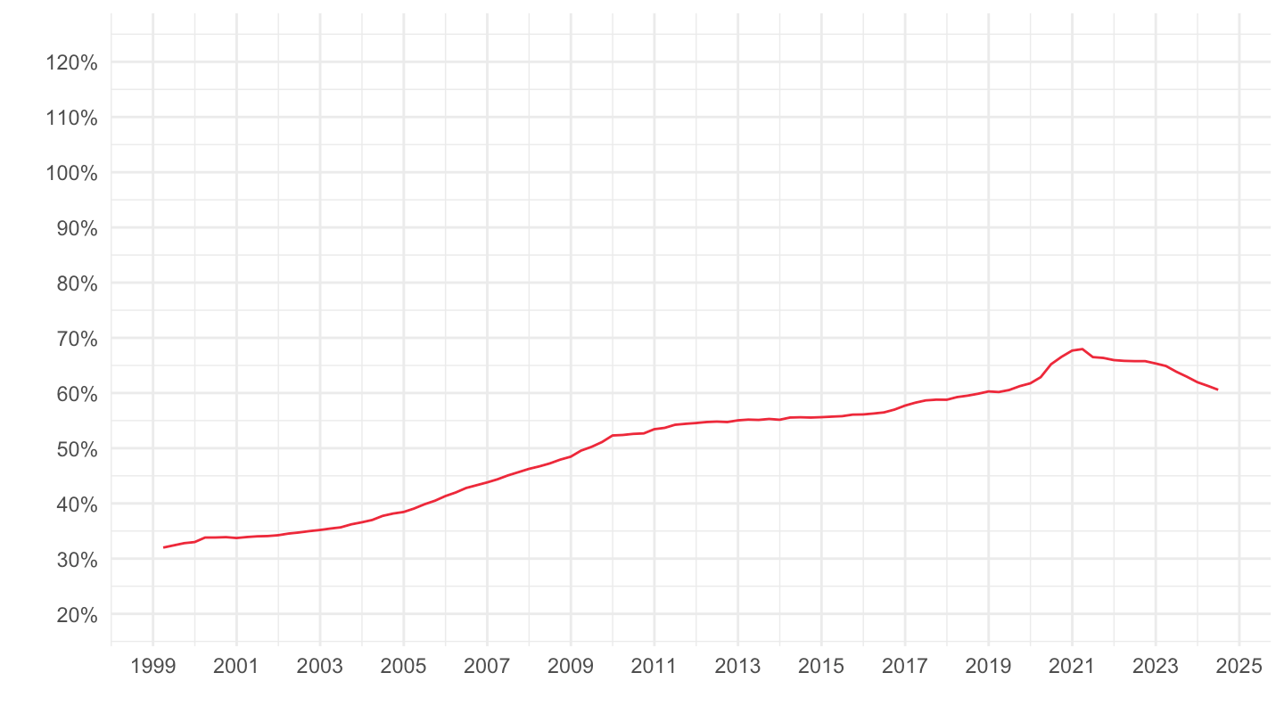
CFT |>


  filter(REF_AREA %in% c("FR", "IT", "DE", "ES", "JP", "I8"),
         INSTR_ASSET == "DETT",
         UNIT_MEASURE == "XDC_R_B1GQ_CY",
         REF_SECTOR == "S1M") |>
  mutate(Ref_area = ifelse(REF_AREA == "I8", "Europe", Ref_area)) |>
  left_join(colors, by = c("Ref_area" = "country")) |>
  mutate(value = value/100) |>
  ggplot() + geom_line(aes(x = date, y = value, color = color)) +
  xlab("") + ylab("") + theme_minimal() + scale_color_identity() + add_6flags +
  scale_x_date(breaks = "2 years",
               labels = date_format("%Y")) +
  scale_y_continuous(breaks = 0.01*seq(-10, 100, 5),
                labels = percent_format(accuracy = 1))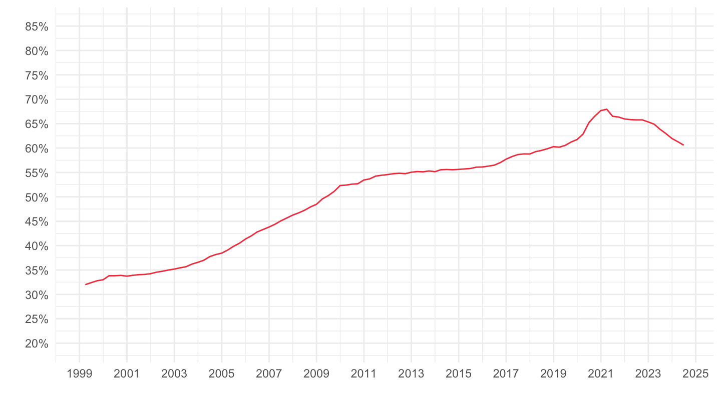
CFT |>


  filter(REF_AREA %in% c("FR", "IT", "DE"),
         INSTR_ASSET == "DETT",
         UNIT_MEASURE == "XDC_R_B1GQ_CY",
         REF_SECTOR == "S1M") |>
  mutate(Ref_area = ifelse(REF_AREA == "I8", "Europe", Ref_area)) |>
  left_join(colors, by = c("Ref_area" = "country")) |>
  mutate(value = value/100) |>
  ggplot() + geom_line(aes(x = date, y = value, color = color)) +
  xlab("") + ylab("") + theme_minimal() + scale_color_identity() + add_3flags +
  scale_x_date(breaks = "2 years",
               labels = date_format("%Y")) +
  scale_y_continuous(breaks = 0.01*seq(-10, 100, 5),
                labels = percent_format(accuracy = 1))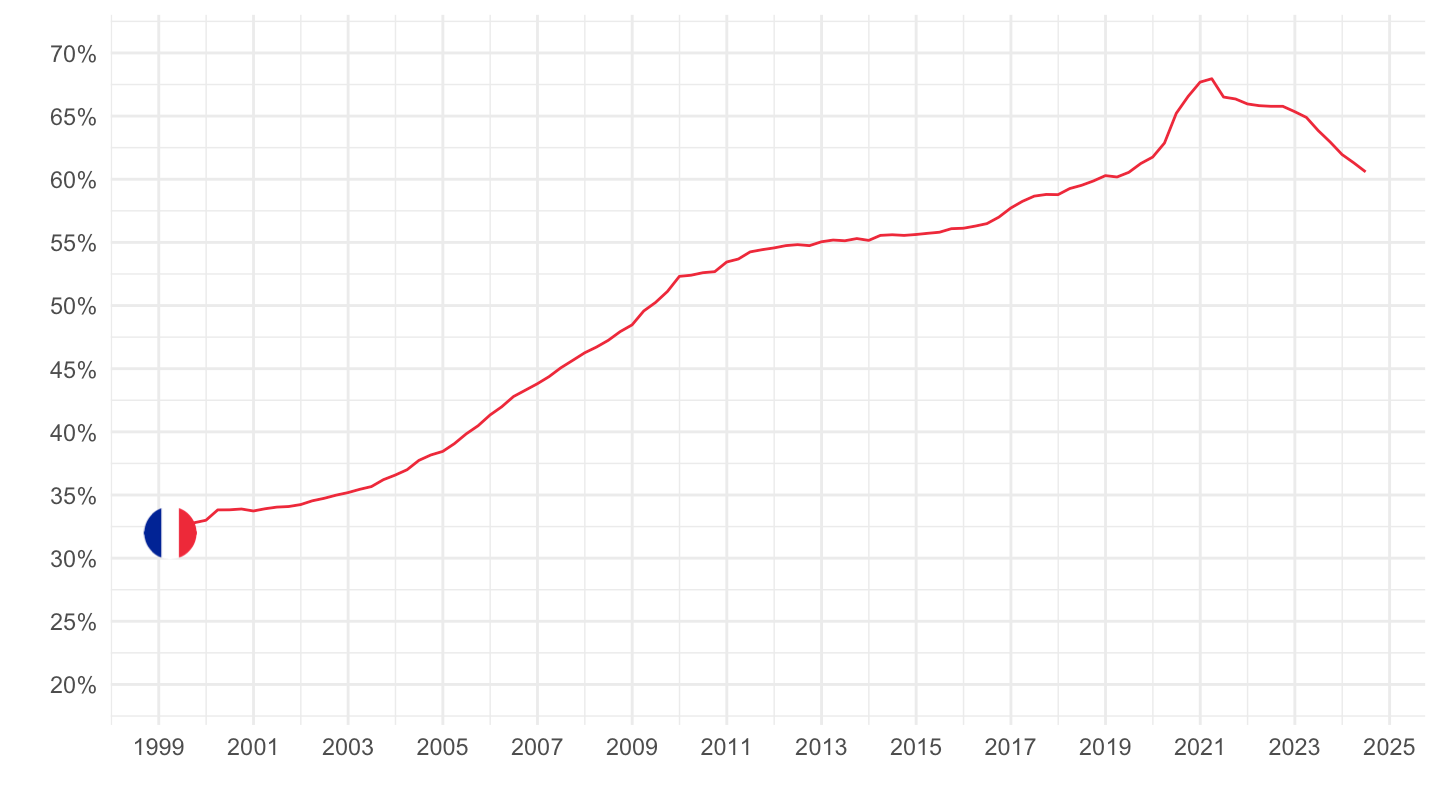
CFT |>


  filter(REF_AREA %in% c("FR", "IT", "DE"),
         INSTR_ASSET == "DETT",
         UNIT_MEASURE == "XDC_R_B1GQ_CY",
         REF_SECTOR == "S1M") |>
  mutate(Ref_area = ifelse(REF_AREA == "I8", "Europe", Ref_area)) |>
  left_join(colors, by = c("Ref_area" = "country")) |>
  mutate(value = value/100) |>
  filter(date >=as.Date("2013-01-01")) |>
  ggplot() + geom_line(aes(x = date, y = value, color = color)) +
  xlab("") + ylab("") + theme_minimal() + scale_color_identity() + add_3flags +
  scale_x_date(breaks = "1 year",
               labels = date_format("%Y")) +
  scale_y_continuous(breaks = 0.01*seq(-10, 100, 2),
                labels = percent_format(accuracy = 1))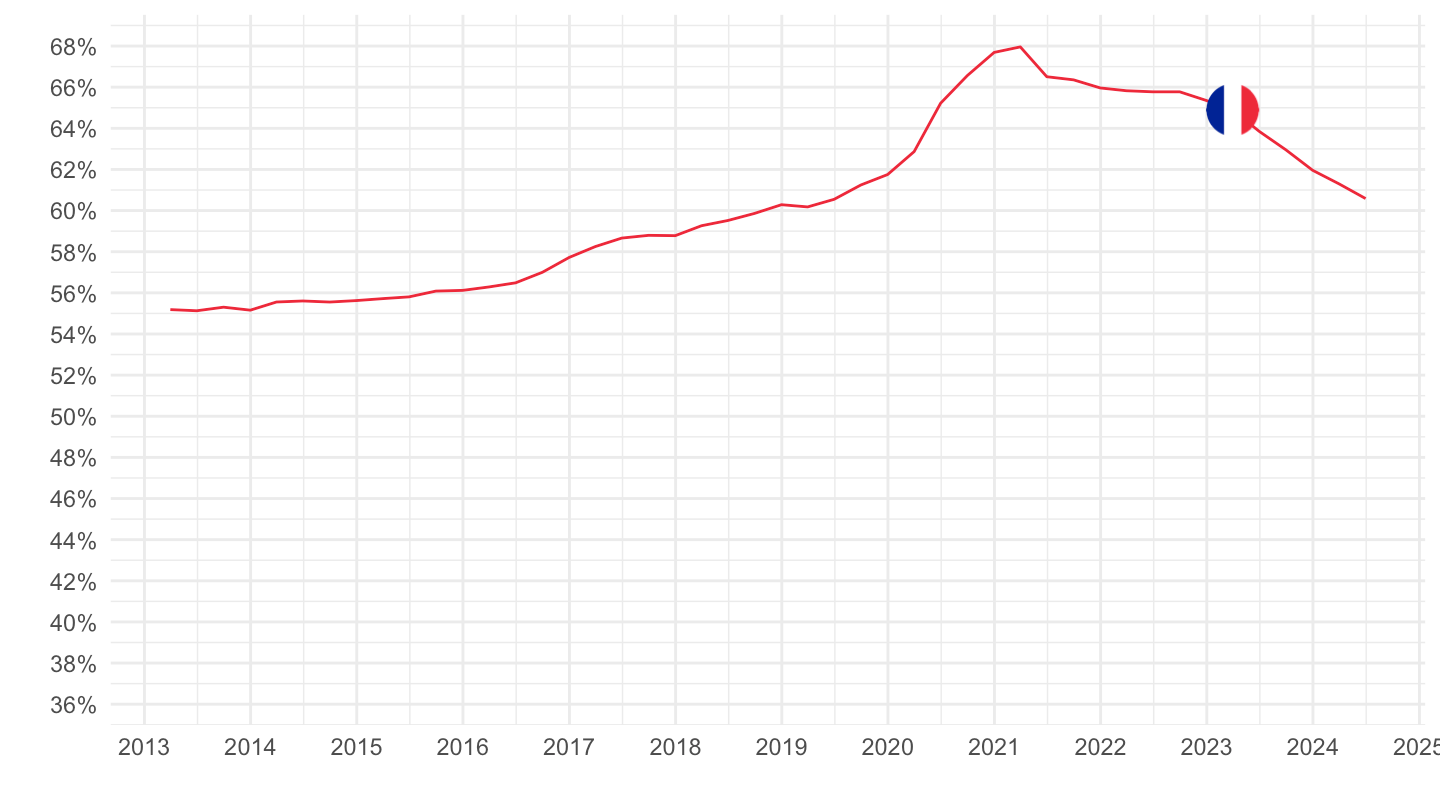
CFT |>


  filter(REF_AREA %in% c("FR", "IT", "DE", "I8"),
         INSTR_ASSET == "DETT",
         UNIT_MEASURE == "XDC_R_B1GQ_CY",
         REF_SECTOR == "S11") |>
  mutate(Ref_area = ifelse(REF_AREA == "I8", "Europe", Ref_area)) |>
  left_join(colors, by = c("Ref_area" = "country")) |>
  mutate(value = value/100) |>
  ggplot() + geom_line(aes(x = date, y = value, color = color)) +
  xlab("") + ylab("") + theme_minimal() + scale_color_identity() + add_4flags +
  scale_x_date(breaks = "2 years",
               labels = date_format("%Y")) +
  scale_y_continuous(breaks = 0.01*seq(-10, 100, 5),
                labels = dollar_format(accuracy = .01, pre = "", su = " année"))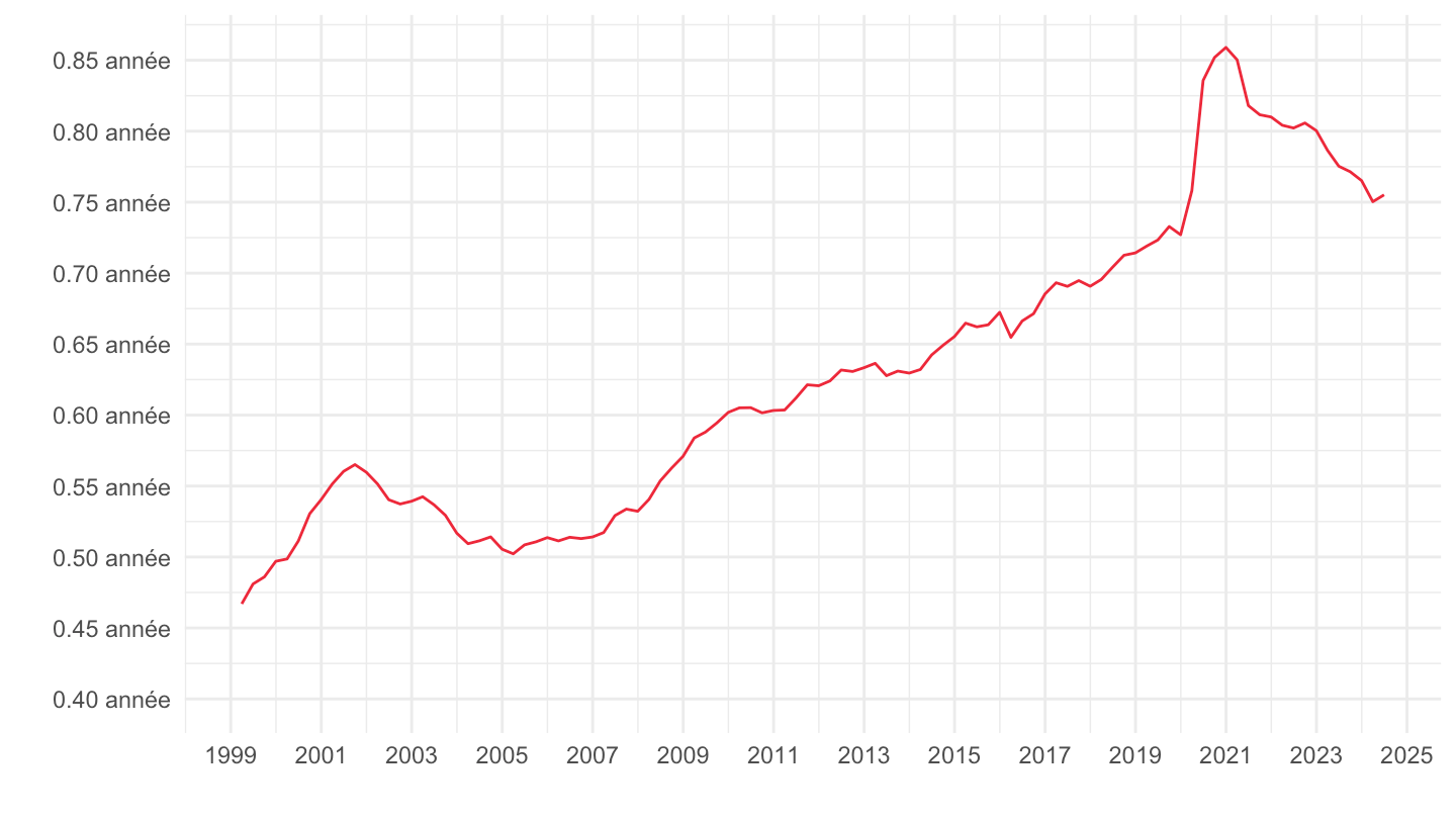
CFT |>

  filter(variable %in% c("CFT.Q.S.FR.W0.S1M.S1.N.L.LE.DETT.T._Z.XDC_R_B1GQ_CY._T.S.V.N._T",
                         "CFT.Q.S.FR.W0.S11.S1.C.L.LE.DETT.T._Z.XDC_R_B1GQ_CY._T.S.V.N._T",
                         "CFT.Q.N.FR.W0.S13.S1.C.L.LE.GD.T._Z.XDC_R_B1GQ_CY._T.F.V.N._T")) |>
  mutate(Variable = gsub(", en % du PIB", "", Variable),
         Variable = gsub(" en % du PIB", "", Variable)) |>
  ggplot() + geom_line(aes(x = date, y = value/100, color = Variable)) +
  xlab("") + ylab("Debt/GDP (in years of GDP)") + theme_minimal() +

  scale_x_date(breaks = "2 years",
               labels = date_format("%Y")) +
  scale_y_continuous(breaks = seq(0, 1.3, 0.1),
                     labels = dollar_format(su = " ans", p = "", acc = 0.1)) +
  theme(legend.position = c(0.3, 0.9),
        legend.title = element_blank(),
        legend.direction = "vertical")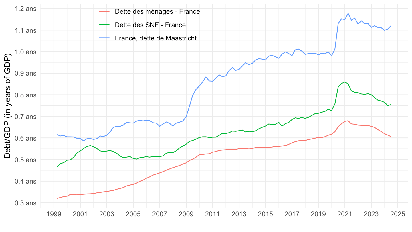
CFT |>

  filter(variable %in% c("CFT.Q.S.FR.W0.S1M.S1.N.L.LE.DETT.T._Z.XDC_R_B1GQ_CY._T.S.V.N._T",
                         "CFT.Q.S.FR.W0.S11.S1.C.L.LE.DETT.T._Z.XDC_R_B1GQ_CY._T.S.V.N._T",
                         "CFT.Q.N.FR.W0.S13.S1.C.L.LE.GD.T._Z.XDC_R_B1GQ_CY._T.F.V.N._T")) |>
  ggplot() + geom_line(aes(x = date, y = value/100, color = Variable)) +
  xlab("") + ylab("") + theme_minimal() +

  scale_x_date(breaks = "2 years",
               labels = date_format("%Y")) +
  scale_y_continuous(breaks = 0.01*seq(-10, 140, 5),
                labels = percent_format(accuracy = 1)) +
  theme(legend.position = c(0.3, 0.9),
        legend.title = element_blank(),
        legend.direction = "vertical")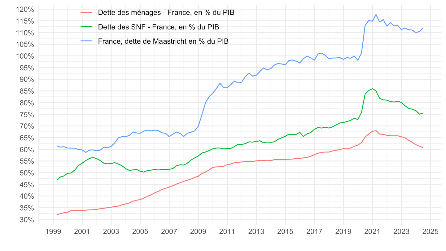
CFT |>

  filter(variable %in% c("CFT.Q.N.DE.W0.S1M.S1.N.L.LE.DETT.T._Z.XDC_R_B1GQ_CY._T.S.V.N._T",
                         "CFT.Q.N.DE.W0.S11.S1.C.L.LE.DETT.T._Z.XDC_R_B1GQ_CY._T.S.V.N._T",
                         "CFT.Q.N.DE.W0.S13.S1.C.L.LE.GD.T._Z.XDC_R_B1GQ_CY._T.F.V.N._T")) |>
  ggplot() + geom_line(aes(x = date, y = value/100, color = Variable)) +
  xlab("") + ylab("") + theme_minimal() +

  scale_x_date(breaks = "2 years",
               labels = date_format("%Y")) +
  scale_y_continuous(breaks = 0.01*seq(-10, 140, 5),
                labels = percent_format(accuracy = 1)) +
  theme(legend.position = c(0.3, 0.9),
        legend.title = element_blank(),
        legend.direction = "vertical")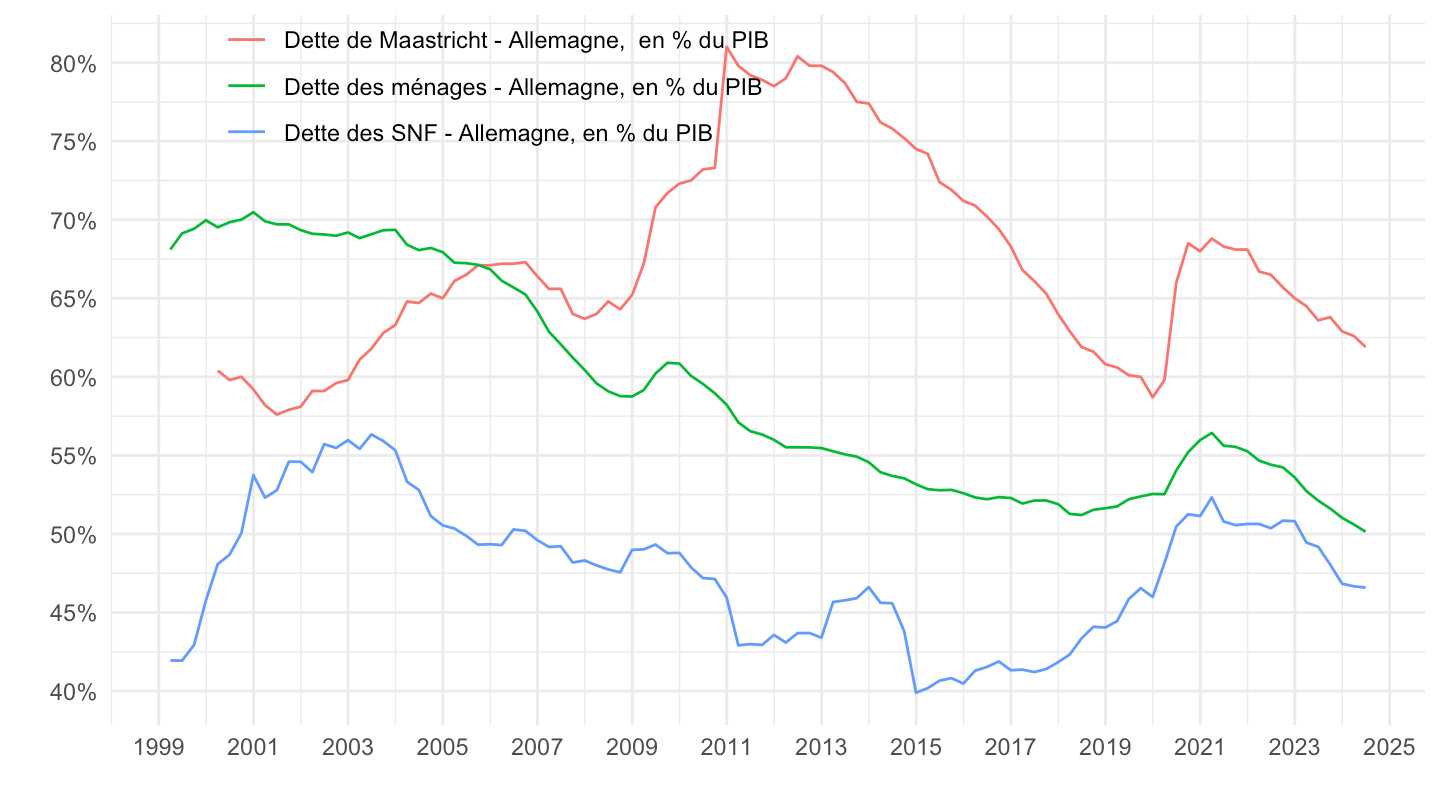
CFT |>

  filter(variable %in% c("CFT.Q.N.IT.W0.S1M.S1.N.L.LE.DETT.T._Z.XDC_R_B1GQ_CY._T.S.V.N._T",
                         "CFT.Q.N.IT.W0.S11.S1.C.L.LE.DETT.T._Z.XDC_R_B1GQ_CY._T.S.V.N._T",
                         "CFT.Q.N.IT.W0.S13.S1.C.L.LE.GD.T._Z.XDC_R_B1GQ_CY._T.F.V.N._T")) |>
  ggplot() + geom_line(aes(x = date, y = value/100, color = Variable)) +
  xlab("") + ylab("") + theme_minimal() +

  scale_x_date(breaks = "2 years",
               labels = date_format("%Y")) +
  scale_y_continuous(breaks = 0.01*seq(-10, 400, 10),
                labels = percent_format(accuracy = 1)) +
  theme(legend.position = c(0.3, 0.9),
        legend.title = element_blank(),
        legend.direction = "vertical")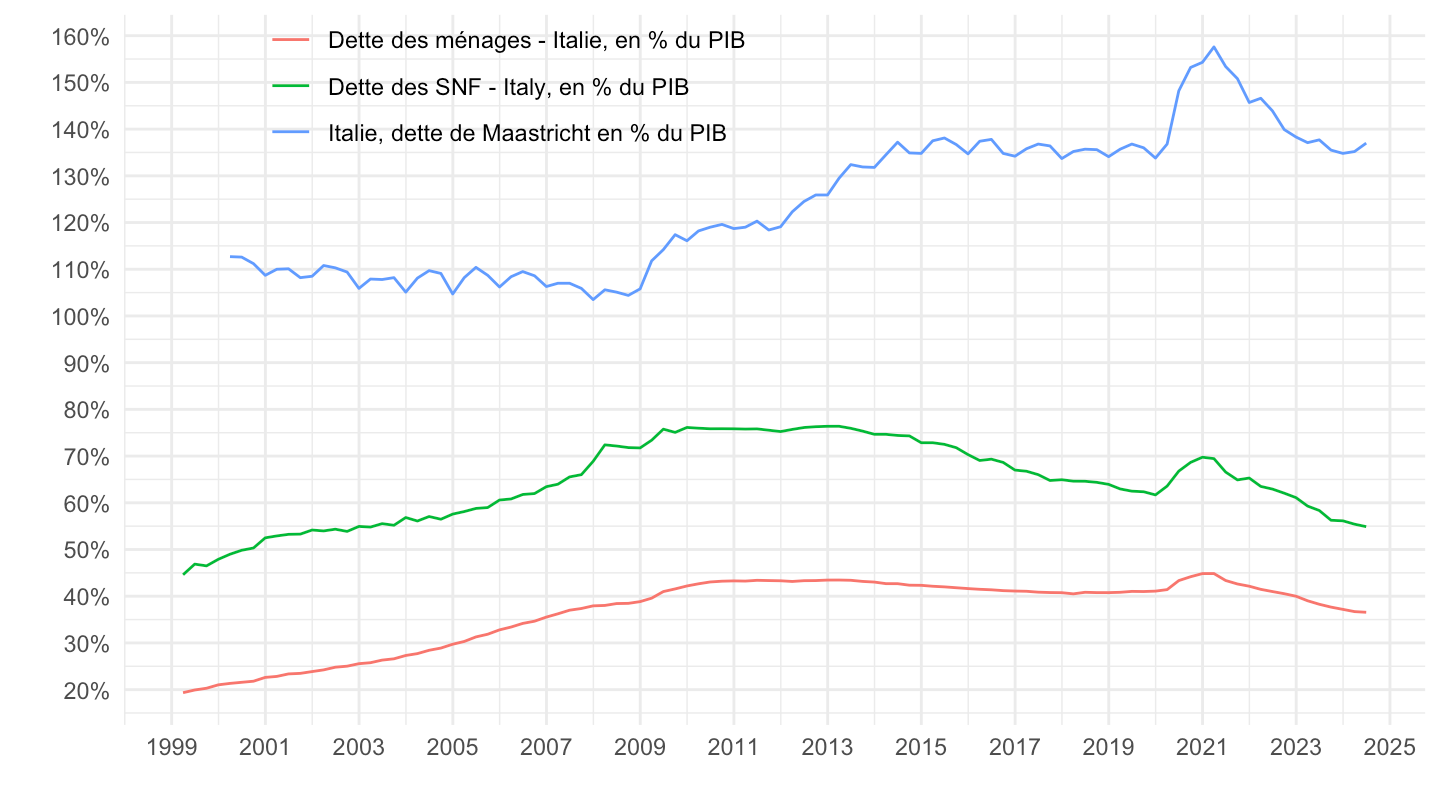
CFT |>

  filter(variable %in% c("CFT.Q.N.ES.W0.S1M.S1.N.L.LE.DETT.T._Z.XDC_R_B1GQ_CY._T.S.V.N._T",
                         "CFT.Q.N.ES.W0.S11.S1.C.L.LE.DETT.T._Z.XDC_R_B1GQ_CY._T.S.V.N._T",
                         "CFT.Q.N.ES.W0.S13.S1.C.L.LE.GD.T._Z.XDC_R_B1GQ_CY._T.F.V.N._T")) |>
  ggplot() + geom_line(aes(x = date, y = value/100, color = Variable)) +
  xlab("") + ylab("") + theme_minimal() +

  scale_x_date(breaks = "2 years",
               labels = date_format("%Y")) +
  scale_y_continuous(breaks = 0.01*seq(-10, 400, 10),
                labels = percent_format(accuracy = 1)) +
  theme(legend.position = c(0.2, 0.9),
        legend.title = element_blank(),
        legend.direction = "vertical")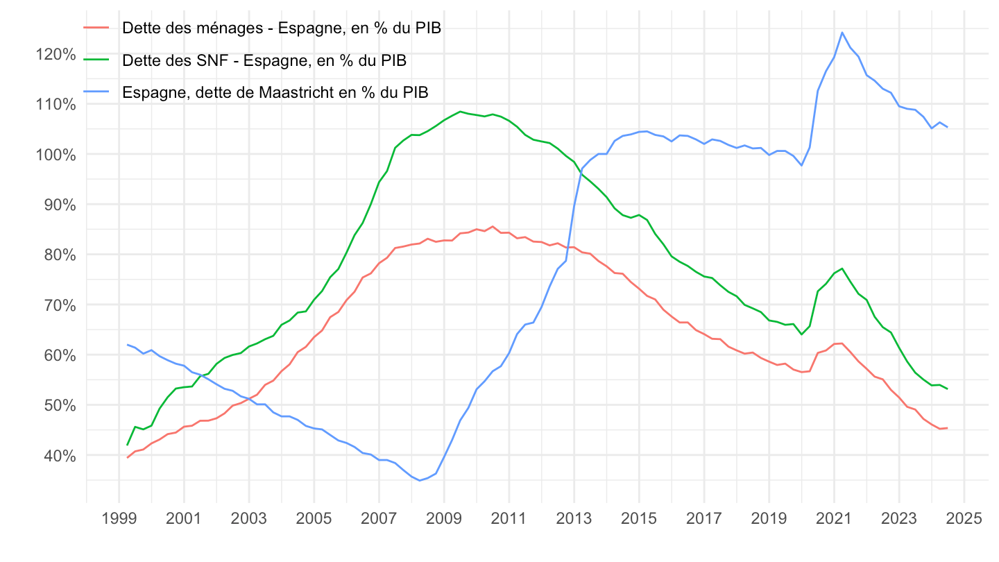
CFT |>

  filter(variable %in% c("CFT.Q.N.I8.W0.S1M.S1.N.L.LE.DETT.T._Z.XDC_R_B1GQ_CY._T.S.V.N._T",
                         "CFT.Q.N.I8.W0.S11.S1.C.L.LE.DETT.T._Z.XDC_R_B1GQ_CY._T.S.V.N._T",
                         "CFT.Q.N.I8.W0.S13.S1.C.L.LE.GD.T._Z.XDC_R_B1GQ_CY._T.F.V.N._T")) |>
  ggplot() + geom_line(aes(x = date, y = value/100, color = Variable)) +
  xlab("") + ylab("") + theme_minimal() +

  scale_x_date(breaks = "2 years",
               labels = date_format("%Y")) +
  scale_y_continuous(breaks = 0.01*seq(-10, 140, 5),
                labels = percent_format(accuracy = 1)) +
  theme(legend.position = c(0.3, 0.9),
        legend.title = element_blank(),
        legend.direction = "vertical")
| source | dataset | Title | Updated |
|---|---|---|---|
| bdf |
CFT | Comptes Financiers Trimestriels - CFT | 2026-08-10 |
 insee insee |
CNA-2014-CONSO-SI | Dépenses de consommation finale par secteur institutionnel - CNA-2014-CONSO-SI | 2026-08-28 |
| insee |
CNA-2014-CSI | Comptes des secteurs institutionnels - CNA-2014-CSI | 2026-08-28 |
| insee |
CNA-2014-FBCF-BRANCHE | Formation brute de capital fixe (FBCF) par branche - CNA-2014-FBCF-BRANCHE | 2026-08-28 |
| insee |
CNA-2014-FBCF-SI | Formation brute de capital fixe (FBCF) par secteur institutionnel - CNA-2014-FBCF-SI | 2026-08-28 |
| insee |
CNA-2014-RDB | Revenu et pouvoir d’achat des ménages - CNA-2014-RDB | 2026-08-28 |
| insee |
CNA-2020-CONSO-MEN | Consommation des ménages - CNA-2020-CONSO-MEN | 2026-08-13 |
| insee |
CNA-2020-PIB | Produit intérieur brut (PIB) et ses composantes - CNA-2020-PIB | 2026-08-28 |
| insee |
CNT-2014-CB | Comptes des branches - CNT-2014-CB | 2026-08-28 |
| insee |
CNT-2014-CSI | Comptes de secteurs institutionnels - CNT-2014-CSI | 2026-08-28 |
| insee |
CNT-2014-OPERATIONS | Opérations sur biens et services - CNT-2014-OPERATIONS | 2026-08-28 |
| insee |
CNT-2014-PIB-EQB-RF | Équilibre du produit intérieur brut - CNT-2014-PIB-EQB-RF | 2026-08-28 |
| insee |
CONSO-MENAGES-2020 | Consommation des ménages en biens - CONSO-MENAGES-2020 | 2026-08-28 |
| insee |
ICA-2015-IND-CONS | Indices de chiffre d'affaires dans l'industrie et la construction - ICA-2015-IND-CONS | 2026-08-28 |
| insee |
conso-mensuelle | Consommation de biens, données mensuelles - conso-mensuelle | 2026-08-02 |
| insee |
t_1101 | 1.101 – Le produit intérieur brut et ses composantes à prix courants (En milliards d'euros) - t_1101 | 2026-08-02 |
| insee |
t_1102 | 1.102 – Le produit intérieur brut et ses composantes en volume aux prix de l'année précédente chaînés (En milliards d'euros 2014) - t_1102 | 2026-08-02 |
| insee |
t_1105 | 1.105 – Produit intérieur brut - les trois approches à prix courants (En milliards d'euros) - t_1105 | 2026-08-02 |
| source | dataset | Title | Updated |
|---|---|---|---|
| bdf |
CFT | Comptes Financiers Trimestriels - CFT | 2026-08-10 |
 bea bea |
T50100 | Table 5.1. Saving and Investment by Sector (A) (Q) - T50100 | 2026-08-28 |
 fred fred |
saving | Saving - saving | 2026-08-28 |
 oecd oecd |
NAAG | National Accounts at a Glance - NAAG | 2026-08-02 |
 wdi wdi |
NY.GDS.TOTL.ZS | Gross domestic savings (% of GDP) - NY.GDS.TOTL.ZS | 2026-08-28 |
| wdi |
NY.GNS.ICTR.ZS | Gross savings (% of GDP) - NY.GNS.ICTR.ZS | 2026-08-28 |